Preprint
Article

Quantifying Uncertainty in Automated Detection of Alzheimer’s Patients Using Deep Neural Network

Altmetrics

Downloads

416

Views

267

Comments

0

Submitted:

08 January 2023

Posted:

09 January 2023

You are already at the latest version

Alerts
Abstract
One of the most common forms of dementia is Alzheimer’s disease (AD), which leads to progressive mental deterioration. Unfortunately, there is no definitive diagnosis and cure that can stop the condition progressing. The diagnosis is often performed based on the clinical history and neuropsychological data, including magnetic resonance imaging (MRI). Deep neural networks (DNN) algorithms are gaining popularity for medical diagnosis, and have been used widely for the analysis of MRI data. DNNs can extract hidden features from thousands of training images automatically. However, they cannot judge how confident they are about their predictions. To use DNNs in safety-critical applications such as medical diagnosis, uncertainty quantification of DNNs predictions is crucial. For this purpose, Monte Carlo dropout (MCD) has been widely used, however, it may lead to overconfident and miss calibrated results. This paper proposes a framework in which the MCD algorithm’s hyper-parameters are optimized during training using Bayesian optimization for the first time. The conducted optimization leads to assigning high predictive entropy to erroneous predictions and making it possible to recognize risky predictions. The proposed framework is used for AD diagnosis, which has not been done before. We compare our method with some existing methods in the literature based on different uncertainty quantification criteria. The results of comprehensive experiments on the Kaggle dataset using a deep model pre-trained on the ImageNet dataset show that the proposed algorithm can quantify uncertainty much better than the existing methods.
Keywords: 
Subject: Computer Science and Mathematics  -   Artificial Intelligence and Machine Learning

I. Introduction

According to the World Health Organization [1], AD is one of the most common causes of dementia, which refers to partial/full loss of mental functioning with adverse effects on activities of daily leaving. AD [2] is a progressive neurological disorder caused by brain deterioration that results in loss of mental functioning, memory, and reasoning. Despite extensive efforts to cure AD, currently, physicians are still unable to stop the disease’s progression or slow down the process of cell destruction in AD patients [3]. Existing treat- ments for AD, therefore, mainly aim to reduce its symptoms, decrease the progression of the disease, and improve quality of life for AD patients. Generally speaking, symptoms of the AD include neurofibrillary tangles and accumulation of plaque amyloids [4]. Such symptoms are, however, observable in healthy individuals reducing their applicability for early diagnosis of AD. While Autopsy can be used for pathological diagnosis, early detection is of significant importance as it can allow timely treatment initiation, reducing the time and cost of clinical trials, establishment of new treatment strategies, and development of more healthy habits in patient’s life [5]. For early detection of AD, clinical imaging tests [6] are, typically, used to identify the degree of nerve damage caused by the AD. In this context, Magnetic Resonance Imaging (MRI) has been widely used as a key imaging modality to observe changes in the structure of the brain. Classification of the AD MRI imaging data is a critical stage in the early detection of AD. In [7], for example, MRI images were used to analyze and classify the synthetic multispectral images and measure the progression of AD. Multilayer perceptron coupled with Kohonen Self-Organized Map (SOM) are used for classification purposes. A 2-degree polynomial was used as the classifier as it is assumed that hyper-quadrics can separate the classes. Due to the high similarity between MRI images of healthy individuals with those of AD patients, however, this is not a trivial classification task. Recently, Jayanthi et al. [8] used Deep Learning (DL) models for such diagnostic classification purposes and achieved human-level results. This has resulted in a surge of interest on development of advanced DL-based models for early detection of AD based on MRI images. Before presenting our contributions in this domain and to better position our work, below, we provide a brief overview of different DL models recently developed for early detection/diagnosis AD.

II. Literature Review

Authors in [9] investigated the effectiveness of different DL- based classification algorithms for the task of AD classification and concluded that Convolutional Neural Network (CNN) is superior to its counterparts. At the same time, several challenges were identified including concerns on shortage of training datasets, high computational complexity, and the need for manual adjustment of hyper-parameters, which can lead to under-fitting or over-fitting of the model. Wang et al. [10] proposed a 3D shufflenet and Principal Component Analysis (PCA) network, where, first, pre-processing is performed on MRI and structural MRI data to eliminate the effects of differences in the size and shape of different people, movement artifacts, and noise. A 3D ShuffleNet is then utilized to extract discriminative features followed by application of the PCANet to analyze the connection of brain function. Finally, the classi- fication process is performed using a Support Vector Machine (SVM). Raees et al. [11] proposed a simple but advanced auto- mated DL pipeline for detecting AD from MRIs of healthy and AD individuals. In the dataset used in this study, 111 people were classified into three classes of Mild Cognitive Impairment (MCI), AD, and normal. For classification purposes, SVM and various DL-based models were tested. The results showed that the DL algorithms offer higher accuracy, ranging from 80% to 90%, in detecting AD. In [12], a DL classifier is proposed based on data collected from more than 217 individuals. An advanced deep CNN model was then used to create a highly generalizable classifier. This model was used as the base model for transfer learning, after which the model was adjusted for AD classification. It achieved 91.3% accuracy in the AD NeuroImaging (ADNI) data set. It also achieved 94.2% and 87.9% accuracy, respectively, on the two unseen independent datasets, Australian Imaging, Biomarkers and Lifestyle (AIBL) and OASIS. Applying the proposed algorithm to brain images of MCI patients showed that the model had three times better performance in predicting whether or not the MCI will progress into AD. In [13], the issue of early detection of MCI with randomized concatenated deep features obtained from two pre-trained models was investigated. The authors proposed a model that simultaneously learns deep features of the brain’s functional networks from MRI images. ResNet18 and DenseNet201 networks have been examined for multi- class AD classification. Accuracy, precision, and recall have been used to evaluate the proposed model. The results showed that the proposed model is able to achieve 98.86%, 98.94%, and 98.89% of accuracy, precision, and recall, respectively, in multi-class classification. In [14], an InceptionV3 CNN architecture was used to predict the diagnosis of AD and MCI. The analysis was performed on two datasets, in which the training process was performed on 90% of one dataset and the test was performed on the remaining 10% of the same set as well as the second data set. The area under the ROC curve of the proposed algorithm was 98%, while the specificity and sensitivity were 82% and 100%, respectively. In [15], a comprehensive investigation was performed for the prediction of AD using biomarkers of various brain images. Multiple biomarking methods of neuroimaging are always better predictors for classifying multiple classes of AD [16]. The proposed study also discussed the open problems that need to be addressed in order to develop an accurate prediction. In [17], using 2,168 MRI images of patients with very mild to various stages of cognitive decline, a solution for faster AD diagnosis was proposed by using DL-based CNN. 10- fold cross-validation was used in which data were divided into 70% as the training data and 30% as the test data for model training and validation. The proposed model in this study successfully classified the various stages of dementia images and achieved an accuracy of 83.3%, which showed better performance compared to other classification techniques such as SVM and logistic regression. Some of the state-of-the- art studies in this field are summarized in Table 1, where the dataset, data type, the applied algorithm, and their performance are listed. It is worth nothing that all the listed works used public datasets except Reference [18].

III. Contributions

Although the above-mentioned studies have focused on ap- plication of DL-based models for diagnosis of AD, uncertainty quantification is overlooked to simplify the modeling task. Failing to properly model uncertainty of DL-based models makes their application questionable in clinical settings as uncertainty quantification is critical to assess overall reliability of the classification pipeline. Located at the intersection of probability, statistics, and computational mathematics, uncer- tainty quantification can determine the confidence level of a model and can show biases caused by overconfidence or uncertainty in the predictions of the model. By enabling uncertainty quantification in the medical models, users can be alerted when a model does not have enough information to make a decision. Consequently, a medical professional can reassess uncertain cases, leading to more confidence in the model. The paper addresses this gap. This paper quantifies the uncertainty of DL-based Classification for Alzheimer’s detection. A solution is provided to improve model uncertainty quantification for AD diagnosis for the first time. In an ideal scenario, high uncertainty is assigned to model predictions whenever the model is not confident about its predictions. In [74], the uncertainty-aware loss function was introduced to improve MCD performance. Although the results were acceptable, performance depends on manual fine-tuning of hyper-parameters. This research proposes a framework capable of determining hyper-parameters using the Bayesian Optimiza- tion (BO) algorithm. The rest of the paper is organized as follows. At first, the most common datasets used in this field are described in Section IV. Then, the proposed method is introduced in detail in Section V. Next, experimental results are explained in Section VI. Finally, we conclude the results in Section VII.

IV. Dataset

There are some public datasets that researchers commonly use. The most famous ones will be described in this section. ADNI [20] was introduced in 2003 as a public-private dataset by principal investigator Michael W. Weiner, MD. The prime motive of this dataset has been to test whether PET, MRI, clinical and neuropsychological assessment, and other biolog- ical markers can be integrated to measure the progression of early AD and mild cognitive impairment (MCI). Researchers utilize and validate data, including PET, MRI scans, CSF, cognitive tests, and blood biomarkers as predictors of the disease. AIBL [64] is another public dataset consisting of AD dementia or mild cognitive impairment (MCI) recruited from tertiary Memory Disorders Clinics or primary-care physicians at two study centers in Perth, Western Australia, Victoria, and Melbourne. The dataset comprised lifestyle, biomarkers, neuroimaging, neuropsychological assessments, and clinical information. Every eighteen months, the follow-up data were collected. Human research ethics committees of Hollywood Private Hospital, Edith Cowan University, St Vincent’s Hos- pital, and Austin Health approved this study. Another public AD dataset is the Open Access Series of Imaging Studies (OA- SIS) [65] which Washington University created. This univer- sity’s AD research center gathered information from demented and non-demented subjects. The dataset consists of both cross-sectional and longitudinal brain MRI scans. The cross- sectional dataset contains details for 416 subjects with ages between 18 and 96 years, while the longitudinal category is comprised of multiple scans of each subject over a time span. Minimal Interval Resonance Imaging in AD (MIRIAD) [66] dataset consists of a longitudinal volumetric T1 MR Images of 23 controls and 46 mild-moderate AD subjects. It is a collection of 708 scans by the same clinician with the same scanner. The sequences were collected at intervals of 2, 6, 14, 26, 38, and 52 weeks, 18 and 24 months. Some information such as Mini-Mental State Examination (MMSE) scores, age, and gender were also collected in this dataset. Computer-aided diagnosis of dementia based on structural (CADDementia) MRI dataset [54] was an image processing challenge defined in 2014. The dataset used in this challenge included 384 MRI images with AD, MCI, and healthy controls. Kaggle dataset [63] consists of 6400, 176×208 MRI images. They are classified into four classes: Non-Demented (ND), Very Mild Demented (VMD), Mild Demented (MID), and Moderate Demented (MOD). In this research, we combined ND and VMD as one group (Group 0) and MID and MOD as another group (Group 1). For this research, we used this dataset.
Table 1. Overview of studies using DL for AD detection.
Ref. Data type Train/Test Method Performance (%)
Liu et al. [19] MRI, PET 10- fold stacked sparse auto-encoders and a softmax regression layer Accuracy 87.76
Liu et al. [21] MRI, PET 10- fold stacked autoencoders and a softmax logistic regressor Accuracy 82.59
Korolev et al. [22] MRI 5 -fold VoxCNN and ResNet Accuracy 80.00
Aderghal et al. [23] sMRI, FuseMe (Method Name) NA 2D CNN Accuracy 85.90
Liu et al. [24] FDG-PET 10- fold 2D CNN and RNNs Accuracy 91.20
Choi et al. [25] FDG-PET, AV-45 PET /V 10- fold 3D CNN Accuracy 96.00
Cheng et al. [26] T1-weighted MR and FDG-PET 10- fold 3D CNN Accuracy 89.64
Wang et al. [27] MRI 50% -50% 2D CNN Accuracy 97.65
Shi et al. [28] MRI, PET, MMSDN 10- fold Multi-modal stacked DPN + SVM Accuracy 97.13
Suk et al. [29] MRI, PET 10- fold Multi-modal DBM + SVM Accuracy 95.35
Suk et al. [30] MRI, PET, CSF 10- fold Stacked AEs + multi-kernel SVM Accuracy 98.80
Payan et al. [31] MRI 5- fold Sparse AEs + 3D CNN Accuracy 95.39
Hosseini-Asl et al. [32] MRI 10- fold 3D CNN Accuracy 99.30
Lu et al. [33] FDG-PET, sMRI 10- fold Multimodal and multiscale DNNs Accuracy 84.60
Sarraf et al. [34] MRI and fMRI 5- fold GoogLeNet + LeNet-5 Accuracy 100
Gupta et al. [35] MRI 75%-25% Sparse AE + CNN Accuracy 94.74
Liu et al. [36] MRI, LDMIL (method) 5- fold 3D CNN Accuracy 91.09
Vu et al. [37] MRI, PET 80%-20% Sparse Autoencoder + 3D CNN Accuracy 91.14
Bi et al. [38] MRI 10- fold 3D CNN+ K means clustering Accuracy 95.52
Puente-Castro et al. [39] Sagittal MRI 80%-20% ANN ResNet + Transfer Learning + SVM Accuracy 86.81
Feng et al. [40] MRI+PET 10- fold fully stacked bidirectional, long short-term memory Accuracy 94.82
Bi et al. [18] EEG spectral images 50%-50% Deep Boltzmann Machine + SVM Accuracy 95.04
Islam et al. [41] MRI 80%-20% Inception-v4 + ResNet F1 Score 90.00
Maqsood et al. [43] MRI 60%-40% AlexNet Accuracy 89.66
Previtali et al. [44] MRI (ORB Method) 10- fold SVM Accuracy 97.00
Hon et al. [45] MRI 5- fold InceptionV4, VGG16 Accuracy 96.25
Ji et al. [46] MRI 60%-40% ResNet50, NASNet, and MobileNet Accuracy 88.37
Zhu et al. [47] sMRI, DA-MIDL (method) 5 -fold Patch-level features, Attention + multi- instance learning Accuracy 89.50
Salvatore et al. [48] MRI 20- fold voxel-level features, Principal Components Analysis Accuracy 76.00
Eskildsen et al. [49] MRI LOOCV ROI-level features, minimal-redundancy-maximal-relevance Accuracy 86.70
Cao et al. [50] MRI 10- fold ROI-level features, multi-kernel + KNN Accuracy 88.60
Tong et al. [51] MRI 10- fold Patch-level Features, multipleinstance-Grap+ SVM Accuracy 90.0
Singh et al. [52] FDG-PET 10- fold PCA+MLP+SVM Accuracy 72.47
Dolph et al. [53] MRI 10- fold stacked AE (SAE) and DNN Accuracy 56.80
Raju et al. [55] sMRI 10- fold 3DCNN with MLP Accuracy 96.66
Cheng et al. [56] MRI-PET 10- fold SAE with elastic net Accuracy 47.00
Karasawa et al. [57] MRI 90%-10% 3D CNN Accuracy 87.00
Ba¨ckstro¨m et al. [58] MRI 60%-40% 3D CNN Accuracy 98.74
Shakeri et al. [59] MRI 80%-20% VAE, MLP Accuracy 84.00
Faturrahman et al. [60] MRI 10- fold DBN Accuracy 91.00
Li et al. [61] MRI 10- fold LSTM-RNN NA
Murugan et al. [62] MRI, DEMNET(method) 80%-20% CNN Accuracy 95.23

V. Prerequisite and Proposed Method

Authors should discuss the results and how they can be interpreted in perspective of previous studies and of the working hypotheses. The findings and their implications should be discussed in the broadest context possible. Future research directions may also be highlighted.This paper quantifies the uncertainty in DL-based classifi- cation for Alzheimer’s detection. A solution is provided to improve model uncertainty quantification for AD diagnosis for the first time. In an ideal scenario, high uncertainty is assigned to model predictions whenever the model is not confident about its predictions. In [67], the uncertainty-aware loss function was introduced to improve MCD performance. Although the results were acceptable, they tunned hyper- parameters by hand. This work proposed a framework capable of determining hyperparameters using the Bayesian optimiza- tion (BO) algorithm. In this section, first, the background knowledge required for the proposed method will be described. Then, the proposed method will be explained in detail.

A. Background

Machine learning models are mainly used for decision- making in different tasks. Quantifying and representing uncer- tainties associated with the predictions are important prereq- uisites for making wise decisions [68]. For example, fallback strategies or further investigations could be triggered if uncer- tainties are high. Despite astonishing performances, machine- based models lack to capture uncertainty [69]. To find these uncertainties, researchers use Bayesian networks. They usually work by assigning distributions to the model parameters (prior distributions) [70]. The input data is used during the training to update the parameters and find the posterior distribution using the Bayes theorem [71]. In D with thousands of parameters, finding the posterior is difficult because of the complexity of finding the marginal likelihood [72]. Different sampling methods have emerged to solve this problem, such as Monte Carlo Markov Chain (MCMC), Gibbs, Hasting, etc. Also, some algorithms can approximate the whole procedure of the Bayesian settings to find the final posterior distribution, such as MCD and Bayesian ensembles.

B. Bayesian network (BN)

A BN is a probabilistic graphical model used to represent knowledge about the uncertain domain. In this network, each node corresponds to a random variable, and each edge corre- sponds to a conditional probability for the corresponding ran- dom variables. It is also known as belief network or Bayesian network. Because of the type of dependencies defined in these types of networks, they can create a directed acyclic graph in which no loops or self-connections are allowed [73].

C. MCD

As mentioned earlier, it is impractical to find the final ditribution of a typical bayesian networks specially with n- dimensional data. Gal [74] proposed that the final distribution could be approximated by performing several forward passes at the test time when dropout is set to on. The predicted mean of the output distribution could be estimated as below:
Preprints 67181 i001
where x represents the test input. The parameters of the model on the tth forward pass are shown by ωˆt, and the conditional probability of y is shown by p(y = c|x, ωˆt). Gal also proposed Predictive Entropy (PE) as a metric for uncertainty in the classification task, by which one could find that how much a specific prediction is related to each class:
Preprints 67181 i002
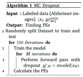
PE shows the deviation of the prediction from its true label. The pseudo-code of the MCD algorithm is available in Algorithm 1.
Preprints 67181 i003

D. Ensemble Networks

Bayesian Ensemble networks (for simplicity we will call it just ensmeble) are another approximation strategies to find the final distribution. As it is obvious from its name, there are several networks trying to predict a specific output. The final distribution (posterior) can be estimated by averaging the mean of networks predictions [75]:
Preprints 67181 i004
where θi is the set of parameters of ith network. The PE for the ensemble is calculated as:
Preprints 67181 i005
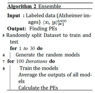
where c represents the number of classes. The psuedo code of this algorithm is shown in Algorithm 2.
Preprints 67181 i006

E. Expected Calibration Error (ECE)

Having well-calibrated predictions is essential for deep neural network models. The concept of ECE was proposed in [76]. The ECE value can be calculated by dividing the output prediction (the output of the softmax) by different groups/bins (here M bins) and calculating the fraction of outputs that are classified correctly and the confidence means (probabilities). The final ECE is equal to the weighted average of the error in all bins:
Preprints 67181 i007
Where n shows the number of samples. The accuracy and the confidence for the mth bin are shown by acc(Bm) and conf(Bm), respectively, and can be calculated as:
Preprints 67181 i008
Preprints 67181 i009
where 1(·) represents the indicator function.

F. The Essence of Knowing Uncertainty

Knowing information associated with the uncertainty gives us an extra insight into our model and where we cannot trust the outcome [77]. Figure 1 shows two brain images of our Alzheimer dataset and their posterior distribution estimated by MCD using 1000 forward passes. Both images are related to people without Alzheimer (Non-Demented). The predicted outcome is obtained by assessing the results related to the softmax output and choosing the bigger mean of the distribution. As it is obvious, if the predictive posterior distribution becomes wide, it would be hard for the model to predict precisely; thus, the model would be less confident. Since the predictive distribution is narrow in Figure 1 (a), the model predicts it as Non-Demented and is sure about its prediction. It should be noted that the narrow posterior distribution corresponds to small PE and vice versa. On the other hand, the model predicts a wrong outcome for Figure 1 (b) and estimates a wide posterior distribution (corresponds to high PE). This way, the model is able to propose its lack of confidence in this specific sample. The he model implies that a second opinion is needed, and the image should be sent to medical experts [78].

G. Proposed Method

The ideal model is able to judge how confident it is about its predictions [79]. To classify the predictions according to their uncertainty, the authors in [80] proposed the idea of the Uncertainty Confusion Matrix (UCM). Using this method, the outcomes can be classified into 4 groups as shown in Figure 2, which is the stepping stone toward the proposal of the uncertainty metrics and which can be used to assess the models objectively:
  • − Uncertainty sensitivity (USen) which could be estimated by dividing the the number of predictions which are in- correct and uncertain by the all the incorrect predictions:
Preprints 67181 i010
  • − Uncertainty Specificity (USpe) which could be obtained by dividing the number of correct and certain predictions by the all number of correct predictions:
Preprints 67181 i011
  • − Uncertainty precision (Upre) that relates to the predic- tions which are incorrect and uncertain dividing by the total number of uncertain prediction:
Preprints 67181 i012
  • − Uncertainty accuracy (Uacc) which is defines as the sum of the predictions located diagonally divided by the total number of predictions:
Preprints 67181 i013
The best scenarios for all the above metrics are near one, and the worst values equal zero. Among all the above metrics, Uacc is the best. According to its definition, the bigger the Uacc, the more the model can differentiate between two classes (correct and incorrect). In other words, the model can handle its uncertainty (can assign high uncertainty to incorrect predictions and vice versa).
Figure 2. The UCM and its components.
Preprints 67181 g002
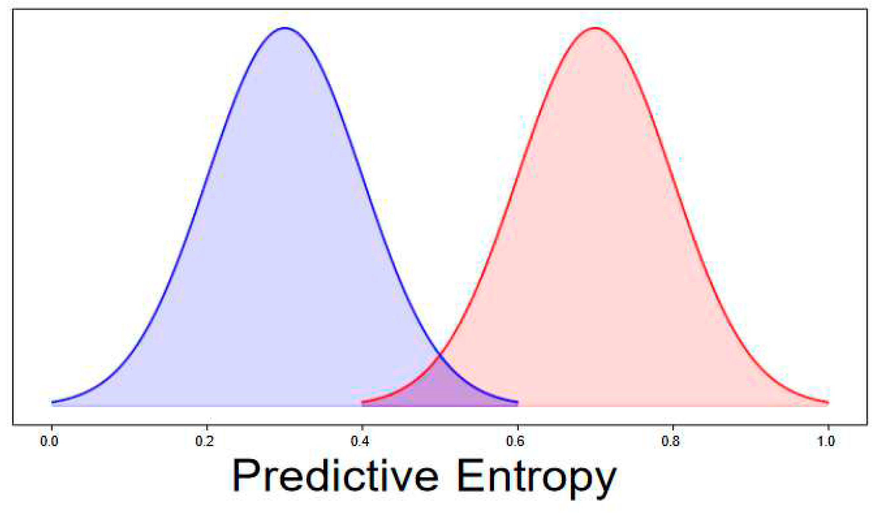
Figure 3 shows a typical distribution of a model’s output. The red distribution is related to the predictions that are classified incorrectly and have high PEs. On the other hand, the blue distribution is related to the predictions that the model classifies correctly and also assigns them low PEs. The high Uacc would equal the situation in which the centers of the two distributions become farther, and the intersections have the least overlap.
Recently, Authors in [67] have proposed an interesting idea for optimizing a simple MCD model, which yielded higher Uacc for the model without sacrificing model accuracy. To this end, a specific loss function is used that takes into account both Uacc and the accuracy of the model:
Loss= Cross Entropy+ Mean of PEs
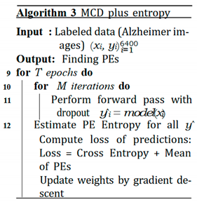
Using the above loss function, the performance of the MCD model is improved. In addition, the pseudo-code summarizing Shamsi et al. [74] method is given in Algorithm 3.
Preprints 67181 i014
In this paper, Shamsi et al.’s framework is improved by optimizing the model hyper-parameters automatically during the training. For hyper-parameters optimization, BO minimizes the loss function in equation 12. In general, there are three hyper-parameter optimization algorithms: BO, grid search, and random search. The two latter algorithms work by sending several queries to the model and finding whether new queries have superiority over previous ones. The major drawback of these algorithms is that they need a substantial amount of time which is not desirable. On the other hand, BO uses the Bayes rule, which assumes a set of hyper-parameters and runs the model to find the posterior distribution. By adding a new sample (input), the hyper-parameter is updated based on a surrogate function. The surrogate function distance with the true distribution is decreased upon the addition of the new sample. Thus, the future decision would be affected by the hyper-parameters chosen in the past. The BO provides a genius algorithm to find the minima using a limited number of steps.

VI. Experimental Results

In this section, we show our algorithm’s results and how it outperforms the previous ones in terms of handling its uncertainty. We divided the dataset into training and test samples. First, these images were resized to 224×224 and normalized. Then, they were given to the convolutional layers of DenseNet121. 50176 convolutional features extracted from DenseNet121 will be provided to two fully connected layers with a softmax. We used the Relu activation function and Adam optimizer. Python programing language and some of its libraries and packages were used, such as Numpy, Pandas, PyTorch, etc to run the experiments. In this paper, we extract the best feature by a DenseNet121 trained on ImageNet dataset. This is because we do not have enough data to train the model or even fine-tune it with some parameters frozen. This limitation can be remedied provided we have access to a large amount of data. Also, we used Google Colab with its default settings to run the experiments (GPU: 1xTesla K80, compute 3.7, 2496 CUDA cores, 12GB GDDR5 VRAM).
The hyperparameters for MCD are 0.25, 0.25, 128, and 64 correspond to P1, P2, L1, and L2 (P represents dropout rate, and L denotes the number of neurons in hidden layers). The features extracted from transfer learning are our new inputs feeding to two fully connected layers (dense layer). Each fully connected (FC) layer consists of a dropout probability (P) and some neurons (L). As the dropout probability plays an important role in MCD algorithm, we propose an automatic framework to capture more reliable uncertainty than the base model in this paper. The researchers usually set these hyper- parameters. However, in this paper, we automatically estimate the best ones to increase the model’s uncertainty accuracy, which will result in capturing more reliable uncertainty. For ensemble, the number of neurons in hidden layers was chosen randomly between (256, 512), (32, 64), respectively. It should note that the hyper-parameters of MCD plus entropy were similar to MCD. After optimization of the MCD with BO considering into account the loss function (MCD plus entropy BO), we have found the following values for hyper-parameters:
Preprints 67181 i015
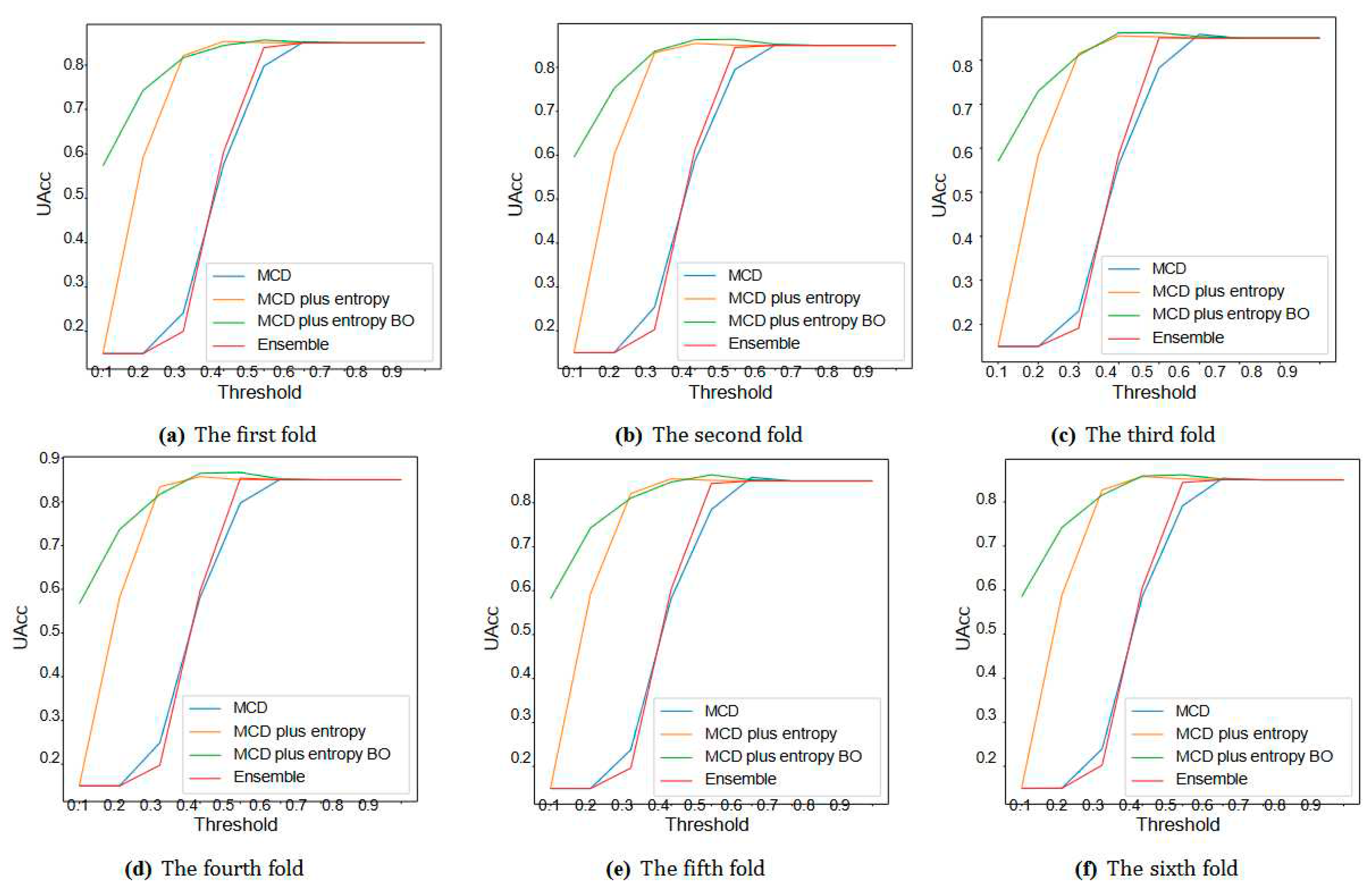
To validate the results, we used 6 folds cross-validation. The Uacc metric for different thresholds is shown in Figure 4. It is obvious that the two optimized MCDs (MCD plus entropy and MCD plus entropy BO) outperform MCD and ensemble. Furthermore, the hyper-parameters optimization helps our al- gorithm outperform the MCD plus entropy.
Uacc and ECE values of four algorithms for different folds are reported in Table 2. It is worth mentioning that ECE shows whether the predictions of a sepecifc model are well-calibrated (the ideal ECE is qual zero). MCD plus entropy BO has the lowest ECE for all the experiments. The Uacc , which shows the capability of the model to differentiate the predictions and assigning high values to wrong predictions and low values to correct ones, is bigger for our proposed framework in each fold than others.
Table 3 reveals the qualitative characteristics of the distri- butions mentioned in Figure 3 and the accuracy for each model for four folds (we just report four folds out of six since there is not enough space in a row to report all six folds). µ1 and µ2 are represents for the estimated centers of the correct and wrong distributions. The distance between these tow is shown by Dist. As mentioned earlier, the bigger the distance between the two distributions and the lesser the intersections, the better the model can handle uncertainty more reliable. The results reported in Table 3 show that our algorithm has minimum distance without sacrificing the model’s accuracy (for some scenarios, the accuracy even has been improved slightly).

A. Discussion

While several studies are available on Alzheimer diagnosis, they all lack the ability to provide uncertainty levels for their predictions. This shortcoming is not acceptable in medical applications. Thus, it is necessary to extend existing deep learning models with uncertainty quantification mechanisms. This is exactly the motivation behind this paper, with special focus on Alzheimer diagnosis. To better understand the im- portance of uncertainty quantification, the proposed method is compared with well-known deep learning methods capable of capturing uncertainty to some extent.
Although the Ensemble method does not utilize Uacc in its training loss function, it has somehow managed to get close to MCD plus Entropy and our method in terms of Uacc. This observation suggests that using multiple classifiers i s similar to fusing the opinions of multiple experts on a specific query. The neural networks have different strengths and weaknesses, so their combination covers the weak points in the decision space and reinforces the strong regions. Another interesting observation can be extracted from Table 4. Given that MCD plus Entropy is the improved version of MCD, the MCD plus Entropy is expected to achieve a higher distance between the distribution of two classes compared to MCD that does not utilize the Cross-Entropy term. However, Table 4 shows counter-intuitive results when the distance rows are compared for MCD and MCD plus Entropy approaches. Despite having the potential to achieve higher performance, MCD plus En- tropy suffers from hand-tuned hyper-parameters, which has apparently hurt performance. Such observation emphasizes the need for automated tuning of hyper-parameters and for automated tuning of hyper-parameters; this is exactly what our method achieves using Bayesian Optimization. Overall, the accuracy of classification h as i ncreased, a nd i ts entropy decreased using our method compared to other methods.

VII. Conclusion

This section is not mandatory, but may be added if there are patents resulting from the work reported in this manuscript.Machine Learning and Artificial intelligence algorithms showed promising ability in prediction medical and biological patterns [81-84], cancer biomarker prediction [85-87], biomedical signal prediction [88-90]. However, uncertainty quantification is a missing part of the current existing models. This paper investigates deep uncertainty quantification tech-niques to detect AD from MRI images. A framework is proposed in which the MCD algorithm can be optimized during training. Consequently, it can assign high predictive entropy to erroneous predictions. In other words, this method can mark risky predictions. We compare our method in terms of quantity and quality with the other three methods in the literature with different uncertainty criteria. The results of comprehensive experiments on the Kaggle dataset already trained by the ImageNet dataset show that the proposed algorithm can quantify reliable uncertainties much better than the existing methods. Furthermore, experimental results show that our proposed algorithm can outperform MCD, MCD plus entropy, and ensemble without sacrificing the model’s accuracy. In other words, this model is able to find wrong predictions. Consequently, these wrong predictions could be sent to medical experts for a second opinion. Hence, we feel that our proposed method will help the clinicians make accurate diagnoses and reduce the possible wrong diagnosis by the automated machine learning models. In future work, different parts of the proposed algorithm can be optimized by different optimization methods. As there are a lot of parameters that must be optimized, meta- heuristic algorithms such as genetic algorithms (GA), particle swarm optimization (PSO), and ant colony optimization (ACO) are suitable options that can be used.

Appendices

Results for two other folds are reported in Table 4.

References

  1. S. Afzal, M. S. Afzal, M. Maqsood, U. Khan, I. Mehmood, H. Nawaz, F. Aadil, O.-Y. Song, and N. Yunyoung, “Alzheimer disease detection techniques and methods: a review,” 2021.
  2. https://www.healthline.com/health/alzheimers-disease/ difference-dementia-alzheimers.
  3. R. N. Bryan, “Machine learning applied to alzheimer disease,” 2016.
  4. S. Kumar, I. S. Kumar, I. Oh, S. Schindler, A. M. Lai, P. R. Payne, and A. Gupta, “Machine learning for modeling the progression of alzheimer disease dementia using clinical data: a systematic literature review,” JAMIA open, vol. 4, no. 3, p. ooab052, 2021.
  5. M. Tanveer, B. M. Tanveer, B. Richhariya, R. U. Khan, A. H. Rashid, P. Khanna, M. Prasad, and C. Lin, “Machine learning techniques for the diagnosis of alzheimer’s disease: A review,” ACM Transactions on Multimedia Computing, Communications, and Applications (TOMM), vol. 16, no. 1s, pp. 1–35, 2020.
  6. E. Pellegrini, L. E. Pellegrini, L. Ballerini, M. d. C. V. Hernandez, F. M. Chappell, V. Gonza´lez-Castro, D. Anblagan, S. Danso, S. Mun˜oz-Maniega, D. Job, C. Pernet, et al., “Machine learning of neuroimaging for assisted diagnosis of cognitive impairment and dementia: a systematic review,” Alzheimer’s & Dementia: Diagnosis, Assessment & Disease Monitoring, vol. 10, pp. 519–535, 2018.
  7. W. P. dos Santos, R. E. W. P. dos Santos, R. E. de Souza, and P. B. dos Santos Filho, “Evaluation of alzheimer’s disease by analysis of mr images using multilayer perceptrons and kohonen som classifiers as an alternative to the adc maps,” in 2007 29th Annual International Conference of the IEEE Engineering in Medicine and Biology Society, pp. 2118–2121, IEEE, 2007.
  8. V. Jayanthi, B. C. V. Jayanthi, B. C. Simon, and D. Baskar, “Alzheimer’s disease clas- sification using deep learning,” in Computational Intelligence and Its Applications in Healthcare, pp. 157–173, Elsevier, 2020.
  9. M. Sethi, S. M. Sethi, S. Ahuja, S. Rani, D. Koundal, A. Zaguia, and W. Enbeyle, “An exploration: Alzheimer’s disease classification based on convolutional neural network,” BioMed Research International, vol. 2022, 2022.
  10. Y. Wang, X. Y. Wang, X. Liu, and C. Yu, “Assisted diagnosis of alzheimer’s disease based on deep learning and multimodal feature fusion,” Complexity, vol. 2021, 2021.
  11. P. M. Raees and V. Thomas, “Automated detection of alzheimer’s disease using deep learning in mri,” in Journal of Physics: Conference Series, vol. 1921, p. 012024, IOP Publishing, 2021.
  12. B. Lu, H.-X. B. Lu, H.-X. Li, Z.-K. Chang, L. Li, N.-X. Chen, Z.-C. Zhu, H.-X. Zhou, X.-Y. Li, Y.-W. Wang, S.-X. Cui, et al., “A practical alzheimer’s disease classifier via brain imaging-based deep learning on 85,721 samples,” Journal of Big Data, vol. 9, no. 1, pp. 1–22, 2022.
  13. M. Odusami, R. M. Odusami, R. Maskeliu¯nas, and R. Damasˇevicˇius, “An intelligent system for early recognition of alzheimer’s disease using neuroimaging,” Sensors, vol. 22, no. 3, p. 740, 2022.
  14. Y. Ding, J. H. Y. Ding, J. H. Sohn, M. G. Kawczynski, H. Trivedi, R. Harnish, N. W. Jenkins, D. Lituiev, T. P. Copeland, M. S. Aboian, C. Mari Aparici, et al., “A deep learning model to predict a diagnosis of alzheimer disease by using 18f-fdg pet of the brain,” Radiology, vol. 290, no. 2, pp. 456–464, 2019.
  15. N. Goenka and S. Tiwari, “Deep learning for alzheimer prediction using brain biomarkers,” Artificial Intelligence Review, vol. 54, no. 7, pp. 4827–4871, 2021.
  16. D. Zhang, D. D. Zhang, D. Shen, A. D. N. Initiative, et al., “Multi-modal multi-task learning for joint prediction of multiple regression and classification variables in alzheimer’s disease,” NeuroImage, vol. 59, no. 2, pp. 895– 907, 2012.
  17. G. Battineni, N. G. Battineni, N. Chintalapudi, F. Amenta, and E. Traini, “Deep learning type convolution neural network architecture for multiclass classification of alzheimer’s disease.,” in BIOIMAGING, pp. 209–215, 2021.
  18. X. Bi and H. Wang, “Early alzheimer’s disease diagnosis based on eeg spectral images using deep learning,” Neural Networks, vol. 114, pp. 119–135, 2019.
  19. S. Liu, S. S. Liu, S. Liu, W. Cai, S. Pujol, R. Kikinis, and D. Feng, “Early diagnosis of alzheimer’s disease with deep learning,” in 2014 IEEE 11th international symposium on biomedical imaging (ISBI), pp. 1015–1018, IEEE, 2014.
  20. “Adni alzheimer‘s disease neuroimaging initiative.” https://adni.loni.usc. edu/.
  21. S. Liu, S. S. Liu, S. Liu, W. Cai, H. Che, S. Pujol, R. Kikinis, D. Feng, M. J. Fulham, et al., “Multimodal neuroimaging feature learning for multiclass diagnosis of alzheimer’s disease,” IEEE transactions on biomedical engineering, vol. 62, no. 4, pp. 1132–1140, 2014.
  22. S. Korolev, A. S. Korolev, A. Safiullin, M. Belyaev, and Y. Dodonova, “Residual and plain convolutional neural networks for 3d brain mri classification,” in 2017 IEEE 14th international symposium on biomedical imaging (ISBI 2017), pp. 835–838, IEEE, 2017.
  23. K. Aderghal, J. K. Aderghal, J. Benois-Pineau, K. Afdel, and C. Gwenae¨lle, “Fuseme: Classification of smri images by fusion of deep cnns in 2d+ ε projec- tions,” in Proceedings of the 15th International Workshop on Content- Based Multimedia Indexing, pp. 1–7, 2017.
  24. M. Liu, D. M. Liu, D. Cheng, W. Yan, and A. D. N. Initiative, “Classification of alzheimer’s disease by combination of convolutional and recurrent neural networks using fdg-pet images,” Frontiers in neuroinformatics, vol. 12, p. 35, 2018.
  25. H. Choi, K. H. H. Choi, K. H. Jin, A. D. N. Initiative, et al., “Predicting cognitive decline with deep learning of brain metabolism and amyloid imaging,” Behavioural brain research, vol. 344, pp. 103–109, 2018.
  26. D. Cheng and M. Liu, “Cnns based multi-modality classification for ad diagnosis,” in 2017 10th international congress on image and sig- nal processing, biomedical engineering and informatics (CISP-BMEI), pp. 1–5, IEEE, 2017.
  27. S.-H. Wang, P. S.-H. Wang, P. Phillips, Y. Sui, B. Liu, M. Yang, and H. Cheng, “Classification of alzheimer’s disease based on eight-layer convolutional neural network with leaky rectified linear unit and max pooling,” Journal of medical systems, vol. 42, no. 5, pp. 1–11, 2018.
  28. J. Shi, X. J. Shi, X. Zheng, Y. Li, Q. Zhang, and S. Ying, “Multimodal neuroimag- ing feature learning with multimodal stacked deep polynomial networks for diagnosis of alzheimer’s disease,” IEEE journal of biomedical and health informatics, vol. 22, no. 1, pp. 173–183, 2017.
  29. H.-I. Suk, S.-W. H.-I. Suk, S.-W. Lee, D. Shen, A. D. N. Initiative, et al., “Hierarchical feature representation and multimodal fusion with deep learning for ad/mci diagnosis,” NeuroImage, vol. 101, pp. 569–582, 2014.
  30. H.-I. Suk and D. Shen, “Deep learning-based feature representation for ad/mci classification,” in International conference on medical image computing and computer-assisted intervention, pp. 583–590, Springer, 2013.
  31. A. Payan and G. a: Montana, “Predicting alzheimer’s disease; arXiv:1502.02506, 2015.
  32. E. Hosseini-Asl, R. E. Hosseini-Asl, R. Keynton, and A. El-Baz, “Alzheimer’s disease diagnostics by adaptation of 3d convolutional network,” in 2016 IEEE international conference on image processing (ICIP), pp. 126–130, IEEE, 2016.
  33. D. Lu, K. D. Lu, K. Popuri, G. W. Ding, R. Balachandar, and M. F. Beg, “Multimodal and multiscale deep neural networks for the early diagnosis of alzheimer’s disease using structural mr and fdg-pet images,” Scientific reports, vol. 8, no. 1, pp. 1–13, 2018.
  34. S. Sarraf, D. D. S. Sarraf, D. D. DeSouza, J. Anderson, G. Tofighi, et al., “Deepad: Alzheimer’s disease classification via deep convolutional neural net- works using mri and fmri,” BioRxiv, p. 070441, 2017.
  35. A. Gupta, M. A. Gupta, M. Ayhan, and A. Maida, “Natural image bases to represent neuroimaging data,” in International conference on machine learning, pp. 987–994, PMLR, 2013.
  36. M. Liu, J. M. Liu, J. Zhang, E. Adeli, and D. Shen, “Landmark-based deep multi- instance learning for brain disease diagnosis,” Medical image analysis, vol. 43, pp. 157–168, 2018.
  37. T. D. Vu, H.-J. T. D. Vu, H.-J. Yang, V. Q. Nguyen, A.-R. Oh, and M.-S. Kim, “Multimodal learning using convolution neural network and sparse autoencoder,” in 2017 IEEE International Conference on Big Data and Smart Computing (BigComp), pp. 309–312, IEEE, 2017.
  38. X. Bi, S. X. Bi, S. Li, B. Xiao, Y. Li, G. Wang, and X. Ma, “Computer aided alzheimer’s disease diagnosis by an unsupervised deep learning technology,” Neurocomputing, vol. 392, pp. 296–304, 2020.
  39. A. Puente-Castro, E. A. Puente-Castro, E. Fernandez-Blanco, A. Pazos, and C. R. Munteanu, “Automatic assessment of alzheimer’s disease diagnosis based on deep learning techniques,” Computers in Biology and Medicine, vol. 120, p. 103764, 2020.
  40. C. Feng, A. C. Feng, A. Elazab, P. Yang, T. Wang, F. Zhou, H. Hu, X. Xiao, and B. Lei, “Deep learning framework for alzheimer’s disease diagnosis via 3d-cnn and fsbi-lstm,” IEEE Access, vol. 7, pp. 63605–63618, 2019.
  41. J. Islam and Y. Zhang, “Early diagnosis of alzheimer’s disease: A neuroimaging study with deep learning architectures,” in Proceedings of the IEEE conference on computer vision and pattern recognition workshops, pp. 1881–1883, 2018.
  42. T. Brosch, R. T. Brosch, R. Tam, A. D. N. Initiative, et al., “Manifold learning of brain mris by deep learning,” in International Conference on Medical Image Computing and Computer-Assisted Intervention, pp. 633–640, Springer, 2013.
  43. M. Maqsood, F. M. Maqsood, F. Nazir, U. Khan, F. Aadil, H. Jamal, I. Mehmood, and O.-y. Song, “Transfer learning assisted classification and detection of alzheimer’s disease stages using 3d mri scans,” Sensors, vol. 19, no. 11, p. 2645, 2019.
  44. F. Previtali, P. F. Previtali, P. Bertolazzi, G. Felici, and E. Weitschek, “A novel method and software for automatically classifying alzheimer’s disease patients by magnetic resonance imaging analysis,” Computer methods and programs in biomedicine, vol. 143, pp. 89–95, 2017.
  45. M. Hon and N. M. Khan, “Towards alzheimer’s disease classification through transfer learning,” in 2017 IEEE International conference on bioinformatics and biomedicine (BIBM), pp. 1166–1169, IEEE, 2017.
  46. H. Ji, Z. H. Ji, Z. Liu, W. Q. Yan, and R. Klette, “Early diagnosis of alzheimer’s disease using deep learning,” in Proceedings of the 2nd International Conference on Control and Computer Vision, pp. 87–91, 2019.
  47. W. Zhu, L. W. Zhu, L. Sun, J. Huang, L. Han, and D. Zhang, “Dual attention multi- instance deep learning for alzheimer’s disease diagnosis with structural mri,” IEEE Transactions on Medical Imaging, vol. 40, no. 9, pp. 2354– 2366, 2021.
  48. R. Cuingnet, E. R. Cuingnet, E. Gerardin, J. Tessieras, G. Auzias, S. Lehe´ricy, M.-O. Habert, M. Chupin, H. Benali, O. Colliot, A. D. N. Initiative, et al., “Automatic classification of patients with alzheimer’s disease from structural mri: a comparison of ten methods using the adni database,” neuroimage, vol. 56, no. 2, pp. 766–781, 2011.
  49. S. F. Eskildsen, P. S. F. Eskildsen, P. Coupe´, D. Garc´ıa-Lorenzo, V. Fonov, J. C. Pruessner, D. L. Collins, A. D. N. Initiative, et al., “Prediction of alzheimer’s disease in subjects with mild cognitive impairment from the adni cohort using patterns of cortical thinning,” Neuroimage, vol. 65, pp. 511–521, 2013.
  50. P. Cao, X. P. Cao, X. Liu, J. Yang, D. Zhao, M. Huang, J. Zhang, and O. Zaiane, “Nonlinearity-aware based dimensionality reduction and over-sampling for ad/mci classification from mri measures,” Computers in biology and medicine, vol. 91, pp. 21–37, 2017.
  51. T. Tong, R. T. Tong, R. Wolz, Q. Gao, R. Guerrero, J. V. Hajnal, D. Rueckert, A. D. N. Initiative, et al., “Multiple instance learning for classification of dementia in brain mri,” Medical image analysis, vol. 18, no. 5, pp. 808– 818, 2014.
  52. S. Singh, A. S. Singh, A. Srivastava, L. Mi, R. J. Caselli, K. Chen, D. Goradia, E. M. Reiman, and Y. Wang, “Deep-learning-based classification of fdg- pet data for alzheimer’s disease categories,” in 13th International Con- ference on Medical Information Processing and Analysis, vol. 10572, pp. 143–158, SPIE, 2017.
  53. C. V. Dolph, M. C. V. Dolph, M. Alam, Z. Shboul, M. D. Samad, and K. M. Iftekharud- din, “Deep learning of texture and structural features for multiclass alzheimer’s disease classification,” in 2017 International Joint Confer- ence on Neural Networks (IJCNN), pp. 2259–2266, IEEE, 2017.
  54. “Caddementia mri dataset.” https://caddementia.grand-challenge.org/.
  55. M. Raju, V. P. M. Raju, V. P. Gopi, and V. Anitha, “Multi-class classification of alzheimer’s disease using 3dcnn features and multilayer perceptron,” in 2021 Sixth International Conference on Wireless Communications, Signal Processing and Networking (WiSPNET), pp. 368–373, IEEE, 2021.
  56. B. Cheng, M. B. Cheng, M. Liu, H.-I. Suk, D. Shen, and D. Zhang, “Multimodal manifold-regularized transfer learning for mci conversion prediction,” Brain imaging and behavior, vol. 9, no. 4, pp. 913–926, 2015.
  57. H. Karasawa, C.-L. H. Karasawa, C.-L. Liu, and H. Ohwada, “Deep 3d convolutional neural network architectures for alzheimer’s disease diagnosis,” in Asian conference on intelligent information and database systems, pp. 287– 296, Springer, 2018.
  58. K. Ba¨ckstro¨m, M. K. Ba¨ckstro¨m, M. Nazari, I. Y.-H. Gu, and A. S. Jakola, “An efficient 3d deep convolutional network for alzheimer’s disease diagnosis using mr images,” in 2018 IEEE 15th International Symposium on Biomedical Imaging (ISBI 2018), pp. 149–153, IEEE, 2018.
  59. M. Shakeri, H. M. Shakeri, H. Lombaert, S. Tripathi, S. Kadoury, A. D. N. Initiative, et al., “Deep spectral-based shape features for alzheimer’s disease clas- sification,” in International Workshop on Spectral and Shape Analysis in Medical Imaging, pp. 15–24, Springer, 2016.
  60. M. Faturrahman, I. M. Faturrahman, I. Wasito, N. Hanifah, and R. Mufidah, “Structural mri classification for alzheimer’s disease detection using deep belief network,” in 2017 11th International Conference on Information & Communication Technology and System (ICTS), pp. 37–42, IEEE, 2017.
  61. H. Li and Y. Fan, “Early prediction of alzheimer’s disease dementia based on baseline hippocampal mri and 1-year follow-up cognitive measures using deep recurrent neural networks,” in 2019 IEEE 16th International Symposium on Biomedical Imaging (ISBI 2019), pp. 368– 371, IEEE, 2019.
  62. S. Murugan, C. S. Murugan, C. Venkatesan, M. Sumithra, X.-Z. Gao, B. Elakkiya, M. Akila, and S. Manoharan, “Demnet: a deep learning model for early diagnosis of alzheimer diseases and dementia from mr images,” IEEE Access, vol. 9, pp. 90319–90329, 2021.
  63. “Kaggle.” https://www.kaggle.com/datasets/tourist55/ alzheimers-dataset-4-class-of-images.
  64. “Aibl australian imaging, biomarkers and lifestyle.” http://aibl.csiro.au.
  65. “Oasis open access series of imaging studies.” http://oasis-brains.org.
  66. “Miriad minimal interval resonance imaging in alzheimer’s disease.” http://ucl.ac.uk/drc/research/methods/ minimalinterval-resonance-imaging-alzheimers-disease-miriad.
  67. A. Shamsi, H. A. Shamsi, H. Asgharnezhad, M. Abdar, A. Tajally, A. Khosravi, S. Nahavandi, and H. arXiv:2110.03260, 2021.
  68. R. Alizadehsani, M. R. Alizadehsani, M. Roshanzamir, M. Abdar, A. Beykikhoshk, M. H. Zangooei, A. Khosravi, S. Nahavandi, R. S. Tan, and U. R. Acharya, “Model uncertainty quantification for diagnosis of each main coronary artery stenosis,” Soft Computing, vol. 24, no. 13, pp. 10149–10160, 2020.
  69. R. Alizadehsani, M. R. Alizadehsani, M. Roshanzamir, M. Abdar, A. Beykikhoshk, A. Khos- ravi, S. Nahavandi, P. Plawiak, R. S. Tan, and U. R. Acharya, “Hybrid genetic-discretized algorithm to handle data uncertainty in diagnosing stenosis of coronary arteries,” Expert Systems, vol. 39, no. 7, p. e12573, 2022.
  70. H. D. Kabir, S. H. D. Kabir, S. Khanam, F. Khozeimeh, A. Khosravi, S. K. Mondal, S. Nahavandi, and U. R. Acharya, “Aleatory-aware deep uncertainty quantification for transfer learning,” Computers in Biology and Medicine, vol. 143, p. 105246, 2022.
  71. H. D. Kabir, A. H. D. Kabir, A. Khosravi, A. Kavousi-Fard, S. Nahavandi, and D. Srini- vasan, “Optimal uncertainty-guided neural network training,” Applied Soft Computing, vol. 99, p. 106878, 2021.
  72. N. Ye and Z. Zhu, “Functional bayesian neural networks for model uncertainty quantification,” 2018.
  73. T. A. Stephenson, “An introduction to bayesian network theory and usage,” tech. rep., Idiap, 2000.
  74. Y. Gal and Z. Ghahramani, “Dropout as a bayesian approximation: Representing model uncertainty in deep learning,” in international conference on machine learning, pp. 1050–1059, PMLR, 2016.
  75. B. Lakshminarayanan, A. B. Lakshminarayanan, A. Pritzel, and C. Blundell, “Simple and scalable predictive uncertainty estimation using deep ensembles,” Advances in neural information processing systems, vol. 30, 2017.
  76. C. Guo, G. C. Guo, G. Pleiss, Y. Sun, and K. Q. Weinberger, “On calibration of modern neural networks,” in International Conference on Machine Learning, pp. 1321–1330, PMLR, 2017.
  77. R. Alizadehsani, M. R. Alizadehsani, M. Roshanzamir, S. Hussain, A. Khosravi, A. Koohes- tani, M. H. Zangooei, M. Abdar, A. Beykikhoshk, A. Shoeibi, A. Zare, et al., “Handling of uncertainty in medical data using machine learning and probability theory techniques: A review of 30 years (1991–2020),” Annals of Operations Research, pp. 1–42, 2021.
  78. M. Raghu, K. M. Raghu, K. Blumer, R. Sayres, Z. Obermeyer, B. Kleinberg, S. Mul- lainathan, and J. Kleinberg, “Direct uncertainty prediction for medical second opinions,” in International Conference on Machine Learning, pp. 5281–5290, PMLR, 2019.
  79. A. Shamsi, H. A. Shamsi, H. Asgharnezhad, S. S. Jokandan, A. Khosravi, P. M. Kebria, D. Nahavandi, S. Nahavandi, and D. Srinivasan, “An uncertainty- aware transfer learning-based framework for covid-19 diagnosis,” IEEE transactions on neural networks and learning systems, vol. 32, no. 4, pp. 1408–1417, 2021.
  80. H. Asgharnezhad, A. H. Asgharnezhad, A. Shamsi, R. Alizadehsani, A. Khosravi, S. Na- havandi, Z. A. Sani, D. Srinivasan, and S. M. S. Islam, “Objective evaluation of deep uncertainty predictions for covid-19 detection,” Scientific Reports, vol. 12, no. 1, pp. 1–11, 2022.
  81. R.Z. Nasab, M.R.E. R.Z. Nasab, M.R.E. Ghamsari, A. Argha, C. Macphillamy, A. Beheshti, R. Alizadehsani, N. Lovell, (2022). Deep Learning in Spatially Resolved Transcriptomics: A Comprehensive Technical View. arXiv:2210.04453.
  82. A. Shoeibi, M. A. Shoeibi, M. Khodatars, M. Jafari, N. Ghassemi, P. Moridian, R. Alizadesani, J.M Gorriz, (2022). Diagnosis of Brain Diseases in Fusion of Neuroimaging Modalities Using Deep Learning: A Review. Information Fusion, 94: 85-113.
  83. H. Alinejad-Rokny, R. H. Alinejad-Rokny, R. Ghavami Modegh, H.R. Rabiee, E. Ramezani Sarbandi, N. Rezaie, K.T. Tam, A.R. Forrest, (2022). MaxHiC: A robust background correction model to identify biologically relevant chromatin interactions in Hi-C and capture Hi-C experiments. PLOS Computational Biology, 18(6): e1010241.
  84. M. Labani, A. M. Labani, A. Afrasiabi, A. Beheshti, N.H. Lovell, (2022). PeakCNV: A multi-feature ranking algorithm-based tool for genome-wide copy number variation-association study. Computational and Structural Biotechnology Journal, 20: 4975-4983.
  85. H. Dashti, I. H. Dashti, I. Dehzangi, M. Bayati, J. Breen, A. Beheshti, N. Lovell, (2022). Integrative analysis of mutated genes and mutational processes reveals novel mutational biomarkers in colorectal cancer. BMC bioinformatics, 23(1): 1-24.
  86. A. Ghareyazi, A. A. Ghareyazi, A. Mohseni, H. Dashti, A. Beheshti, I. Dehzangi, H.R. Rabiee, (2021). Whole-genome analysis of de novo somatic point mutations reveals novel mutational biomarkers in pancreatic cancer. Cancers, 13(17): 4376.
  87. M. Bayati, H.R. M. Bayati, H.R. Rabiee, M. Mehrbod, F. Vafaee, D. Ebrahimi, A.R. Forrest, (2020). CANCERSIGN: a user-friendly and robust tool for identification and classification of mutational signatures and patterns in cancer genomes. Scientific reports, 10(1): 1-11.
  88. M. Hosseinpoor, H. M. Hosseinpoor, H. Parvin, S. Nejatian, V. Rezaie, K. Bagherifard, A. Dehzangi, (2020). Proposing a novel community detection approach to identify cointeracting genomic regions. Mathematical Biosciences and Engineering, 17(3): 2193-2217.
  89. H. Alinejad-Rokny, E. H. Alinejad-Rokny, E. Sadroddiny, V. Scaria, (2018). Machine learning and data mining techniques for medical complex data analysis. Neurocomputing, 276(1).
  90. A. Argha, B.G. A. Argha, B.G. Celler, N.H. Lovell, (2022). Blood Pressure Estimation from Korotkoff Sound Signals Using an End-to-End Deep-Learning-Based Algorithm. IEEE Transactions on Instrumentation and Measurement, 71: 1-10.
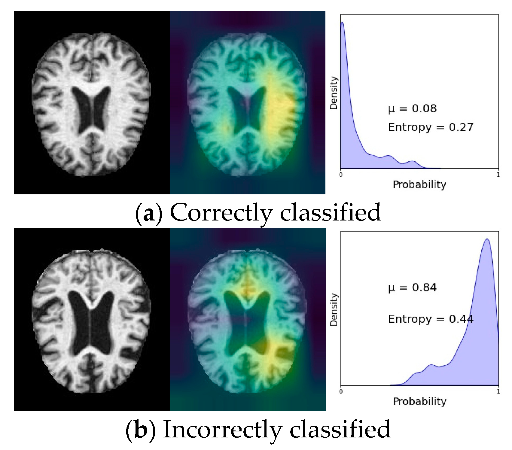
Figure 1. Two sample of Non Demented images from Alzheimer dataset and their posterior ditributions based on MCD algorithm. µ is the center of the distribution.
Preprints 67181 g001
Figure 3. The output of the model is classified to two distributions based on the predictive entropy.
Preprints 67181 g003
Figure 4. UA metric for different algorithms for different folds of data.
Preprints 67181 g004
Table 2. Uacc and ECE values of four algorithms for different folds.
UQ Method Fold = 1 Fold = 2 Fold = 3 Fold = 4 Fold=5 Fold = 6
Uacc ECE Uacc ECE Uacc ECE Uacc ECE Uacc ECE Uacc ECE
MCD 78.3 12.1 80.4 9.71 79.3 9.5 78.1 9.6 78.4 9.74 79.5 9.9
MCD plus entropy 85 1.3 85.25 5.9 85 6.3 85.2 4.85 85.2 4.9 85 5
MCD plus entropy BO 85.2 1.04 86.3 3.06 86.4 3.31 85.7 3.09 86.2 2.9 85.9 3.2
ensemble 84.6 9.2 84.68 5.9 84 8.9 84.5 8.9 84.5 8.9 83.9 9.3
Table 3. The characteristics of output distributions are depicted while the accuracy is almost 85% The centers of the correct and incorrect distributions (µ1 and µ2) and the distance between them (Dist) are shown.
UQ Method Fold = 1 Fold = 2 Fold = 3 Fold = 4
µ1 µ2 Dist Acc µ1 µ2 Dist Acc µ1 µ2 Dist Acc µ1 µ2 Dist Acc
MCD 0.417 0.470 0.053 85.06 0.400 0.503 0.103 85 0.404 0.506 0.102 85 0.405 0.503 0.097 85
MCD plus entropy 0.190 0.231 0.041 85.06 0.207 0.296 0.089 85 0.209 0.301 0.092 85 0.208 0.295 0.087 85
MCD plus entropy BO 0.103 0.180 0.077 85.06 0.147 0.340 0.192 85 0.149 0.352 0.203 85 0.147 0.339 0.191 85
ensemble 0.404 0.441 0.037 85.06 0.390 0.454 0.064 85 0.391 0.453 0.063 85 0.393 0.453 0.060 85
Table 4. Rusults for two other folds.
UQ Method Fold = 5 Fold = 6
µ1 µ2 Dist Acc µ1 µ2 Dist Acc
MCD 0.404 0.496 0.092 85.02 0.404 0.494 0.090 85
MCD plus entropy 0.208 0.287 0.079 85.02 0.209 0.282 0.073 85
MCD plus entropy BO 0.148 0.329 0.181 85.02 0.149 0.316 0.167 85
ensemble 0.392 0.450 0.058 85.02 0.391 0.448 0.057 85
Disclaimer/Publisher’s Note: The statements, opinions and data contained in all publications are solely those of the individual author(s) and contributor(s) and not of MDPI and/or the editor(s). MDPI and/or the editor(s) disclaim responsibility for any injury to people or property resulting from any ideas, methods, instructions or products referred to in the content.
Copyright: This open access article is published under a Creative Commons CC BY 4.0 license, which permit the free download, distribution, and reuse, provided that the author and preprint are cited in any reuse.
Prerpints.org logo

Preprints.org is a free preprint server supported by MDPI in Basel, Switzerland.

Subscribe

© 2024 MDPI (Basel, Switzerland) unless otherwise stated