1. Introduction
Emotions are part of everyone’s daily life as they are crucial to many aspects: They are a significant factor in human interactions, influence decision-making, and are involved in mental health. Emotions play a crucial role in human communication and cognition, which makes comprehending them significant to understanding human behaviour [
1]. The field of affective computing strives to build systems that can recognize and interpret human affects [
1,
2], offering exciting possibilities for education, entertainment, and healthcare. Giving machines emotional intelligence could, for instance, facilitate early detection and prediction of (mental) diseases or their symptoms since specific emotional and affective states are often indicators thereof [
3]. For example, long-term stress is one of today’s significant factors causing health problems, including high blood pressure, cardiac diseases, and anxiety [
4]. Notably, some patients with epilepsy (PWE) report premonitory symptoms or auras as specific affective states, stress, or mood changes, enabling them to predict an oncoming seizure [
5]. The association of premonitory symptoms and seizure counts has been analyzed from patient reported diaries [
6], and the non-pharmacological interventions proved to reduce the seizure rate [
7]. However, many PWE can not consistently identify their prodromal symptoms, and many do not perceive prodromes [
8], emphasizing the necessity of objective prediction of epileptic seizures. In previous work, the authors proposed developing a system to predict seizures by continuously monitoring their affective states [
9]. Therefore, measuring and predicting affective states in real-time through neurophysiological data could aid in finding pre-emptive therapies for epilepsy patients by identifying the pre-ictal state to predict a seizure onset. That would be incredibly beneficial, especially to people with drug-resistant epilepsy, and improve their quality of life by enabling them to anticipate and mitigate possibly violent seizures [
3,
8]. Consequently, emotion detection in this paper is motivated by the idea that allowing computers to perceive and understand human emotions could improve human-computer interaction (HCI) and enhance their abilities to make decisions by adapting their reactions accordingly.
Since emotional reactions are seemingly subjective experiences, neurophysiological biomarkers, such as heart rate, respiration, or brain activity [
10,
11] are inevitable. Additionally, for continuous monitoring of affective states and thus detecting or predicting stress-related events reliably, low-cost consumer-grade devices rather than expensive and immobile hospital equipment would be more meaningful [
12]. It is an important area of interest in cognitive science and affective computing, with use cases varying from designing brain-computer interfaces [
13,
14] to improving healthcare for patients suffering from neurological disorders [
15,
16]. Among these, Electroencephalography (EEG) has proven to be an accurate and reliable modality without needing external annotation [
17,
18]. With recent advancements in wearable technology, consumer-grade EEG devices have become more accessible and reliable, opening possibilities for countless real-life applications. Wearable EEG devices like the
Emotiv EPOC Neuroheadset or the
Muse S headband have become quite popular tools in emotion recognition [
19,
20,
21].
Muse S headband has also been used for event-related potential (ERP) research [
12] and for the challenge of affect recognition in particular. More specifically,
Muse S has already been used in experimental setups to obtain EEG data from which the mental state (relaxed/concentrated/neutral) [
13], and the emotional state (using the valence-arousal space) [
22], could be reliably inferred through the use of a properly trained classifier.
However, a challenging but important step to identifying stress-related events or improving HCI in real-life settings is to recognise changes in peoples’ affect by leveraging live data. The EEG-based emotion classification mentioned in the literature has nearly exclusively employed traditional machine learning strategies, i.e., offline classifiers, often combined with complex data preprocessing techniques, on static datasets, making it unsuitable for daily monitoring. Therefore, researchers are interested in building a real-time emotion classification pipeline since lately, where the classification results are obtained from pre-recorded (and already preprocessed) data, often utilizing a pre-trained model [
23,
24] rather than working with (live) data streams. Li et al. [
25] address the challenges when a model can see the data only once by leveraging cross-subject and cross-session data but does not apply live incoming data stream to their work. Whereas Lan et al. [
26] analyse stable features for real-time emotion recognition and implement their proposed algorithm in two emotion-monitoring applications where computer avatars reflect a person’s emotion based on live EEG data. However, the live emotion classification is based on a static model, which has to be trained in a prior training session and is not updated afterward. To the best of our knowledge, only Nandi et al. [
27] have employed online learning to classify emotions from an EEG data stream from the DEAP dataset and proposed an application scenario in e-learning but did not report on undertaking any such live experiments. Indeed, more research is needed on using online machine learning for emotion recognition.
Moreover, multi-modal labeled data for the prediction of affective states have been made freely available through annotated affective databases, like DEAP [
28], DREAMER [
29], ASCERTAIN [
30], and AMIGOS [
21], which play a significant role in further enhancing the research of this field. They include diverse data from experimental setups using differing emotional stimuli like music, videos, pictures, or cognitive load tasks in an isolated or social setting. Such databases enable the development and improvement of frameworks and model architectures with existing data of ensured quality. However, none of the datasets have published the data collection framework to be reused in curating the data from wearable EEG devices in live settings.
Therefore, firstly, the key contribution of this paper is the establishment of a lightweight emotion classification pipeline that can provide predictions on a person’s affective state based on an incoming EEG data stream in real-time, efficiently enough to be used in real applications i.e., seizure prediction. The developed pipeline leverages online learning to train subject-specific models on data streams by implementing binary classifiers for the affect dimensions: Valence and Arousal. The pipeline is validated by streaming the existing datasets of established quality, AMIGOS, with better predictive performance than state-of-the-art contributions. Secondly, an experimental framework is developed, similar to the AMIGOS dataset, which can collect neurophysiological data from a wide range of commercially available EEG devices and show live prediction of the subjects’ affective states even when labels arrive with a delay. Data from 15 participants were captured by using two consumer-grade devices. Thirdly, the most novel contribution of this paper is to validate the pipeline on the curated dataset by wearable EEG devices in the first experiment with consistent prediction performance with the AMIGOS dataset. Following this, the live prediction was performed successfully on an incoming data stream in the second experiment with delayed incoming labels.
The curated data from the experiments and metadata is accessible to the designated researchers as per the participants’ consent; therefore, the dataset is available upon request for scientific use via a contact form on Zenodo (
https://doi.org/10.5281/zenodo.7398263 ). The Python code for loading the dataset and implementations of the developed pipeline are made available on GitHub (
https://github.com/HPI-CH/EEGEMO). The next section will explain the material and methods utilized within this paper following the results and discussion sections.
4. Discussion
In this paper, firstly, a real-time emotion classification pipeline was built for binary classification (high/low) of the two affect dimensions
Valence and
Arousal. Adaptive Random Forest (ARF), Streaming Random Patches (SRP), and Logistic Regression (LR) classifiers with 10-fold cross-validation were applied to the EEG data stream. The subject-dependent models were evaluated with progressive and delayed validation, respectively, when immediate and delayed labels were available. The pipeline was validated on the existing data of ensured quality from the state-of-the-art AMIGOS [
21] dataset. By streaming the recorded data to the pipeline, the mean F1-Score achieves more than 80% for both ARF and SRP models. The results outperform the authors’ baseline results by approximately 25% and are also slightly better than the work reported by [
64] using the same dataset. Topic et al. [
65] shows a better performance; however, due to the reported complex setup and computationally costly methods, the system is unsuitable for real-time emotion. Nevertheless, the results mentioned in the related work apply offline classifiers with a hold-out or a k-fold cross-validation technique. In contrast, our pipeline applies an online classifier by employing progressive validation. To the best knowledge, no other work tested an online EEG-based emotion classification framework on the published AMIGOS dataset.
Secondly, a similar framework from the AMIGOS dataset was established within this paper which can collect neurophysiological data from a wide range of neurophysiological sensors. In this paper, two consumer-grade EEG devices were used to collect data from 15 participants while watching 16 emotional videos. The framework available in the mentioned repository can be adapted for similar experiments.
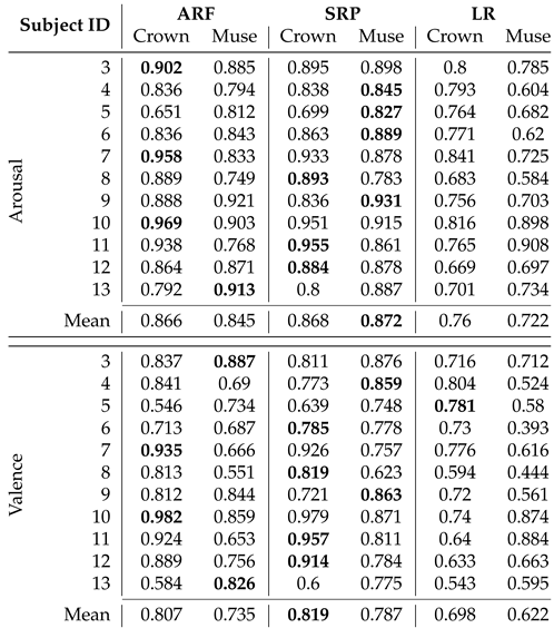
Thirdly and most importantly, we curated data in two experiments to validate our classification pipeline using the mentioned framework. 11 participants took part in Experiment I, where EEG data was recorded while watching 16 emotion elicitation videos. The pre-recorded data is streamed to the pipeline and showed a mean F1-Score of more than 82% with ARF and SRP classifiers using progressive validation. The finding validates the competence of the pipeline on the challenging dataset coming from consumer-grade EEG devices. Additionally, the online classifiers consistently showed better performance for ARF and SRP than LR on all compared modalities. However, internal testing verifies that the run-time on the training step of the pipeline of ARF is less than that of SRP, concluding to use of ARF in live prediction. The analysis on window length shows a clear trend of increasing performance scores with decreasing window length; therefore, a window length of 1 second is chosen for further analysis. Although the two employed consumer-grade devices possess a different number of sensors at contrasting positions, there were no statistically significant differences between the achieved performance scores on their respective data found. Therefore, we used both devices for live prediction, and the pipeline was applied to a live incoming data stream in Experiment II with the above-mentioned features of the model. In the first part of the experiment, the model is trained with the immediate labels from the EEG data stream. In the second part, the model is used to predict affect dimensions while the labels are available after a delay of the video length. The model is continuously updated whenever a new label is available. The performance scores achieved during the live classification with delayed labels are much lower than with immediate labels in Experiment I, motivating to induce artificial delay to the data stream from Experiment I. The results are compatible with the results from the live prediction. The literature reports better results for real-time emotion classification frameworks [
23,
24,
26] with the assumption of knowing the true label immediately after a prediction. The novelty of this paper is to present a real-time emotion classification pipeline close to the realistic production scenario from daily life with the possibility of including further modifications in future work.
As a future work, the selected stimuli can be shortened to reduce the delay of the incoming labels so that the model is updated more frequently. Otherwise, multiple intermediate labels can also be included in the study design to ensure the inclusion of short time emotions felt while watching the movies. Furthermore, more dynamic preprocessing of the data can be included with feature selection algorithms for better prediction in live settings. Moreover, the collected data from the experiments reveal a strong class imbalance in the self-reported affect ratings for arousal, with high arousal ratings making up 82.96% of all ratings in that dimension.This general trend towards more high arousal ratings is also visible in the AMIGOS dataset, albeit not as intensely (62.5% high arousal ratings). In contrast, Betella et al. [
46] found “a general desensitization towards highly arousing content” in participants. The underrepresented class can be upsampled in the model training in the future, or the basic emotions can be classified instead of arousal and valance, solving a multiclass problem [
66]. Including more participants in the future for live prediction, the prediction can be visible to the participant as well to include neurofeedback. It will also be interesting to see if the predictive performance improves by utilizing additional modalities other than EEG, for example, Heart rate, Electrodermal activity [
19,
22,
28].
Figure 1.
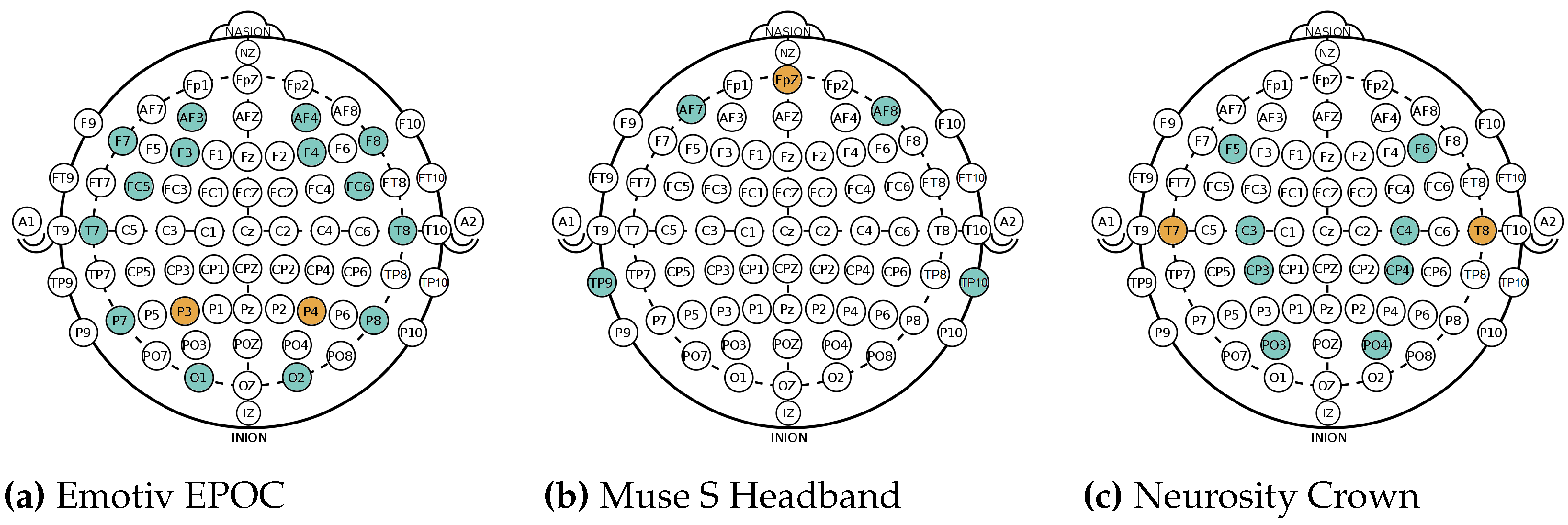
Different electrode positions, according to the international 10-20 system, of the EEG devices used in AMIGOS dataset: (a), and in Experiments I and II: (b,c) . Sensor locations are marked in blue, references in orange.
Figure 1.
Different electrode positions, according to the international 10-20 system, of the EEG devices used in AMIGOS dataset: (a), and in Experiments I and II: (b,c) . Sensor locations are marked in blue, references in orange.
Figure 2.
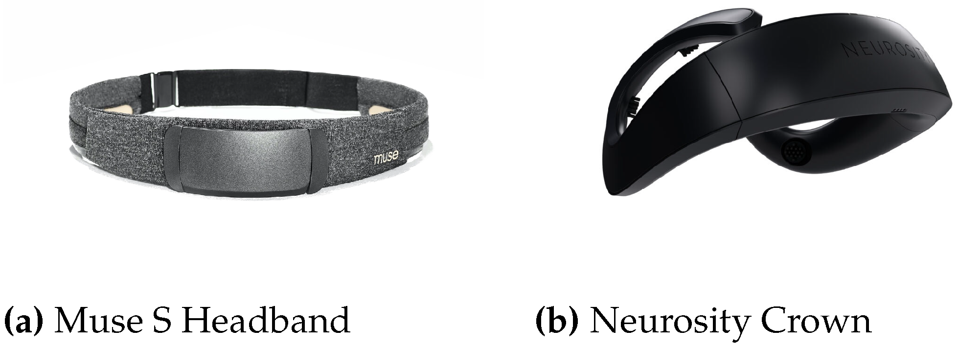
Two consumer-grade EEG devices with integrated electrodes used in the experiments.
Figure 2.
Two consumer-grade EEG devices with integrated electrodes used in the experiments.
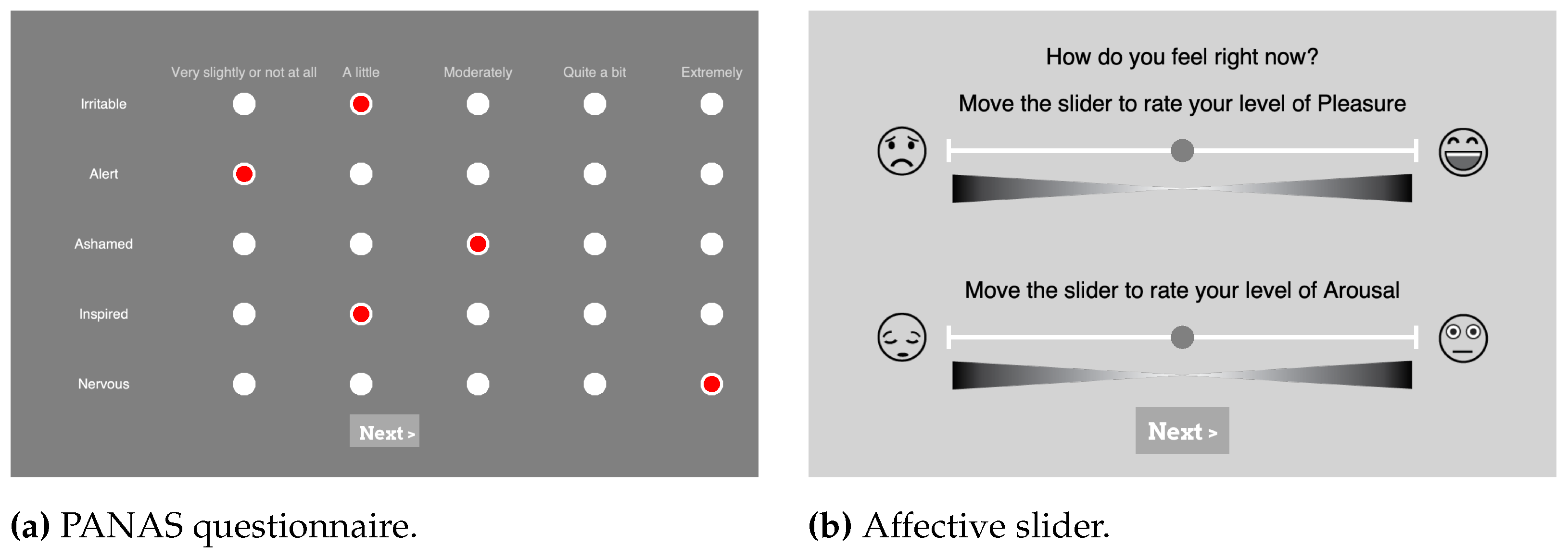
Figure 3.
Screenshots from the PsychoPy [
34] experimental setup of self-assessment questions the participants were shown in Experiment I and II. (
a) is one part of the PANAS questionnaire with 5 different levels represented by clickable radio buttons with levels explanation on top. (
b) shows the AS for valence displayed on top and the slider for arousal on the bottom.
Figure 4.
(
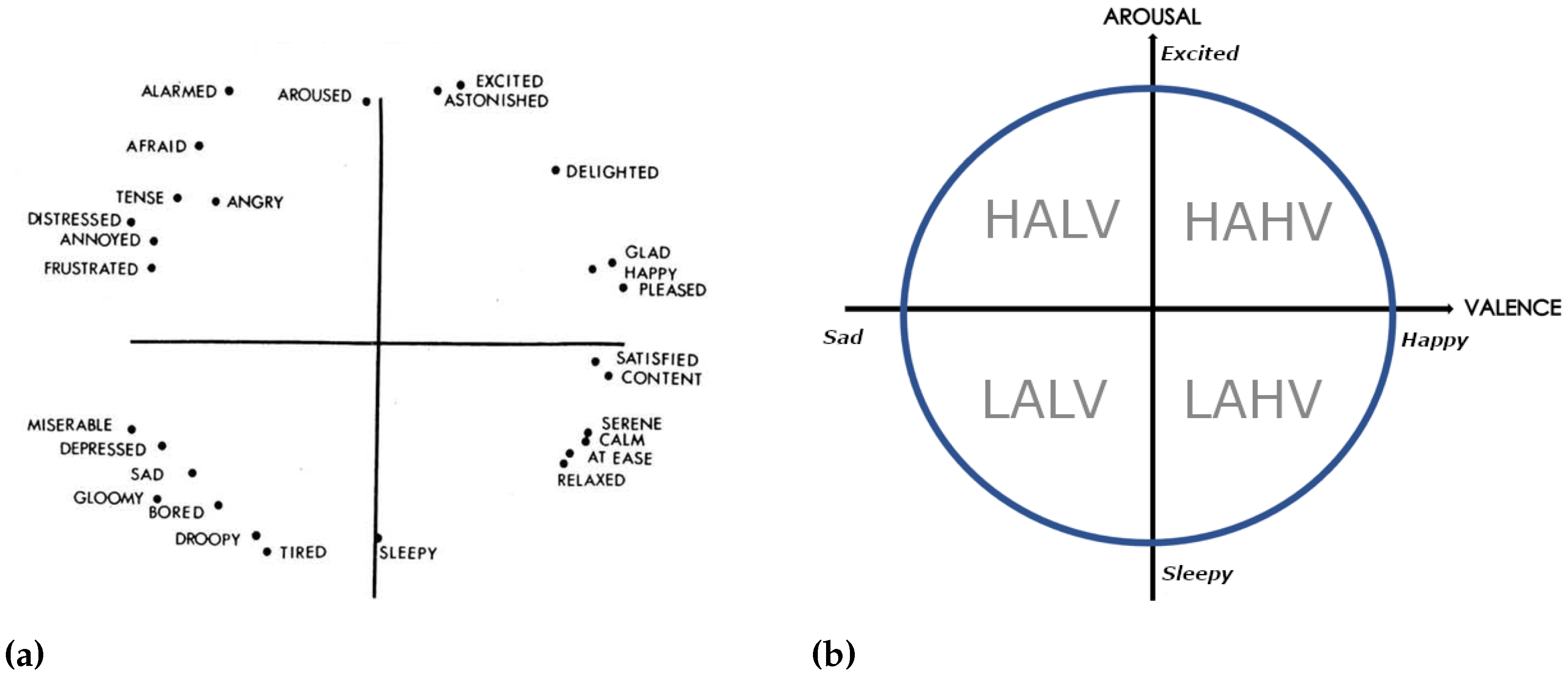
a) Russell’s Circumplex Model of Affect in multidimensional scaling [
43], 28 affect words are placed on the plane spanned by two axes without explicit title. (
b) is a reduced version of Russell’s Circumplex Model of Affect [
44] depicting the valence-arousal space as it is used in this work with the four quadrants: HALV, HAHV, LAHV, LALV. H, L, A, and V stand for high, low, arousal and valence respectively.
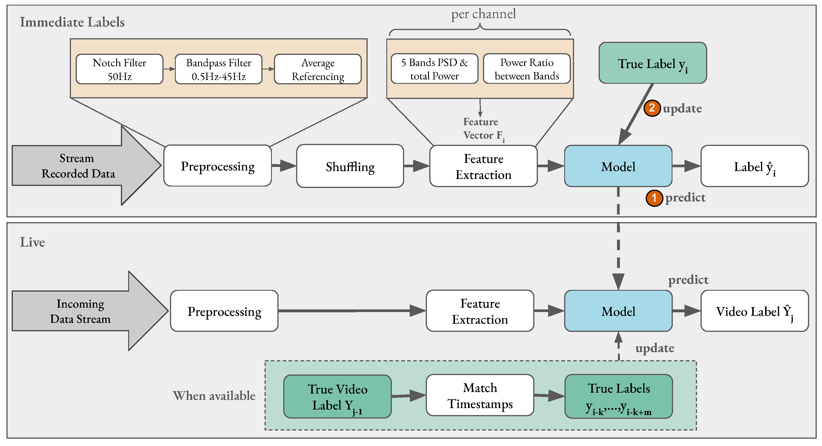
Figure 5.
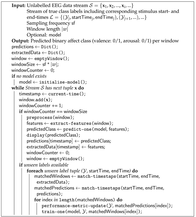
Overview of pipeline steps for affect classification. The top grey rectangle shows the pipeline steps employed in an immediate label setting with prerecorded data. For each extracted feature vector the model (1) first predicts its label before (2) being updated with the true label for that sample. In the live setting, the model is not updated after every prediction, as the true label of a video only becomes available after the stimuli has ended. The timestamp of the video is matched to the samples’ timestamps to find all samples that fell into the corresponding time frame and update the model with their true labels.
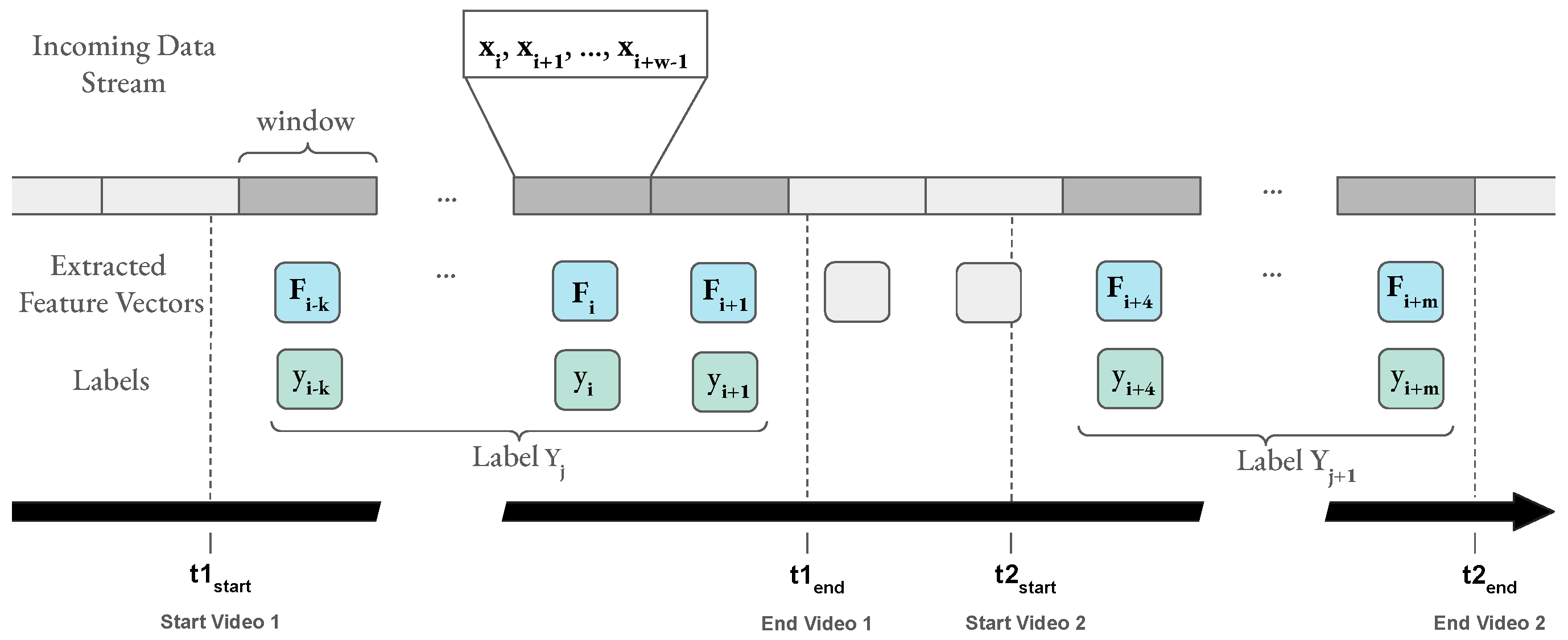
Figure 6.
The incoming data stream is processed in tumbling windows (grey rectangles). One window includes all samples arriving during a specified time period, e.g., 1 second. The pipeline extracts one feature vector per window. Windows during a stimulus (video) are marked in dark grey. Participants rated each video with one label per affect dimension . All feature vectors extracted from windows that fall into the time frame of a video (between and of that video) receive a label corresponding to the reported label of that video. If possible, the windows are aligned with the end of the stimulus, otherwise, all windows that lie completely inside a video’s time range are considered.
Figure 7.
(a) Progressive validation incorporated into the basic flow of the training process (`test-then-train’) of an online classifier in an immediate label setting. ( represents an input feature vector and its corresponding label. (b) Evaluation incorporated into the basic flow of the training process of an online classifier when labels arrive delayed.
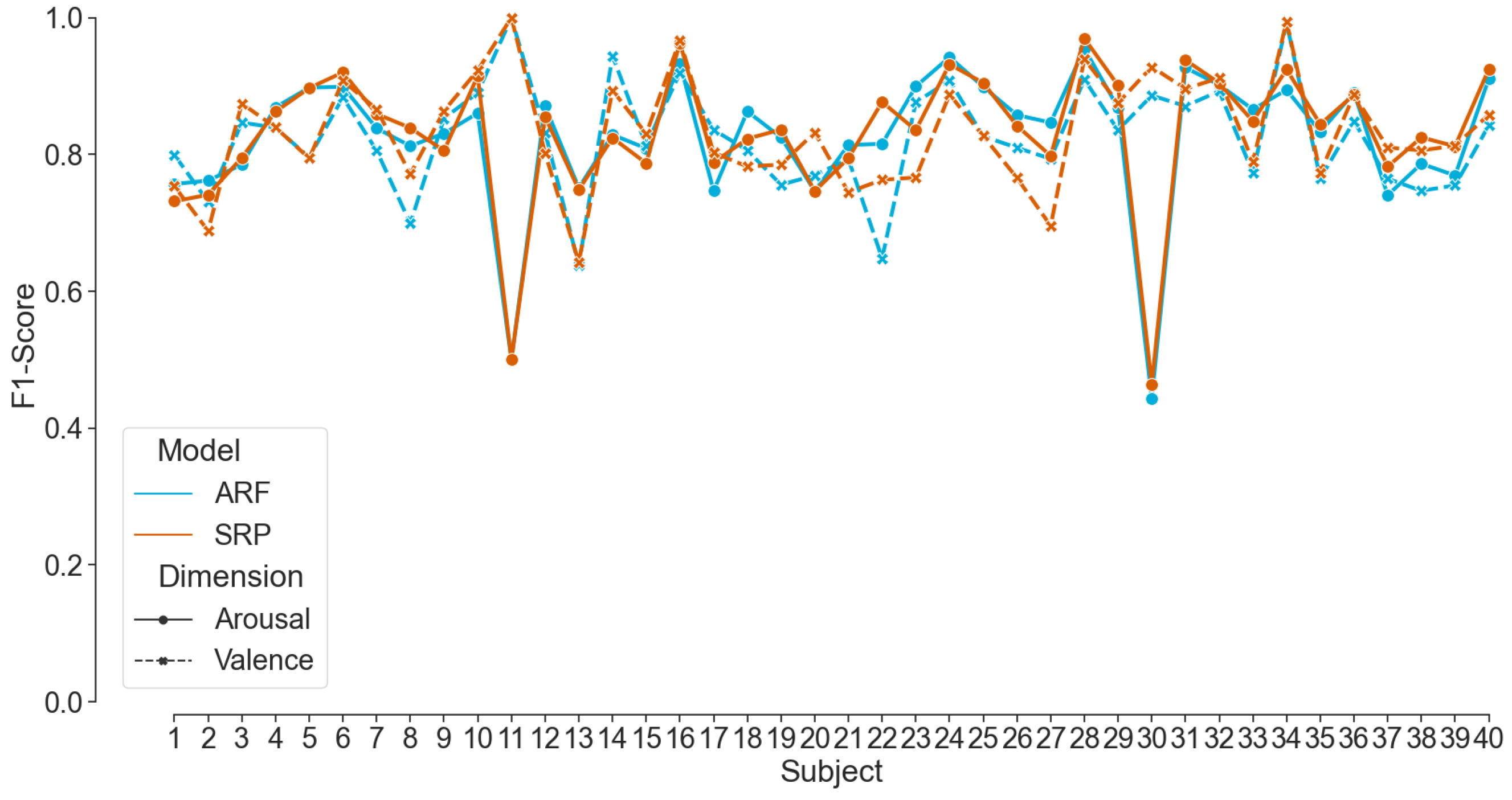
Figure 8.
F1-Score for Valence and Arousal classification achieved by ARF and SRP per participant in the AMIGOS dataset.
Figure 8.
F1-Score for Valence and Arousal classification achieved by ARF and SRP per participant in the AMIGOS dataset.
Figure 9.
Mean F1-Score achieved by ARF, SRP, and LR over the whole dataset for both affect dimension with respect to window length.
Figure 9.
Mean F1-Score achieved by ARF, SRP, and LR over the whole dataset for both affect dimension with respect to window length.
Table 1.
The source movies of the videos used in the experiments are listed per quadrant in the valence-arousal space. Video IDs are stated in parentheses, sources marked with a † were taken from the MAHNOB-HCI dataset [
41]; all the others stem from DECAF [
40]. In the category column, H, L, A, and V stand for high, low, arousal, and valence respectively. This table has been adapted from Miranda-Correa et al. [
21].
| Category |
Source Movie |
| HAHV |
Airplane (4), When Harry Met Sally (5), Hot Shots (9), Love Actually (80)†
|
| LAHV |
August Rush (10), Love Actually (13), House of Flying Daggers (18), |
| |
Mr Beans’ Holiday (58)†
|
| LALV |
Gandhi (19), My Girl (20), My Bodyguard (23), The Thin Red Line (138)†
|
| HALV |
Silent Hill (30)†, Prestige (31), Pink Flamingos (34), Black Swan (36) |
Table 2.
Number of channels and derived features for each device: Muse Headband: 64 features; Neurosity Crown: 128 features; Emotiv EPOC: 224 features.
Table 2.
Number of channels and derived features for each device: Muse Headband: 64 features; Neurosity Crown: 128 features; Emotiv EPOC: 224 features.
| Device |
# Channels |
# Derived Features |
| Muse Headband |
4 |
64 |
| Neurosity Crown |
8 |
128 |
| Emotiv EPOC |
14 |
224 |
Table 3.
Comparison of mean F1-Scores and accuracy of Valence and Arousal recognition on the AMIGOS dataset for short videos over all participants for different classifiers. Gray color represents the results from this paper. NR stands for not reported.
Table 3.
Comparison of mean F1-Scores and accuracy of Valence and Arousal recognition on the AMIGOS dataset for short videos over all participants for different classifiers. Gray color represents the results from this paper. NR stands for not reported.
| Study or Classifier |
F1-Score |
Accuracy |
| Valence |
Arousal |
Valence |
Arousal |
| LR |
0.669 |
0.65 |
0.702 |
0.688 |
| ARF |
0.825 |
0.826 |
0.82 |
0.846 |
| SRP |
0.834 |
0.831 |
0.826 |
0.847 |
| Miranda-Correa et al. [21] |
0.576 |
0.592 |
NR |
NR |
| Siddharth et al. [64] |
0.8 |
0.74 |
0.83 |
0.791 |
| Topic et al. [65] |
NR |
NR |
0.874 |
0.905 |
Table 4.
Comparison of mean F1-Scores of Arousal and Valence recognition per participant and device from Experiment I with three classifiers using progressive validation. Bold values indicate the best performing model per participant and dimension. The mean total represents the calculated average of all models’ F1-Scores.
Table 5.
F1-Score and accuracy for the live affect classification in Experiment II (part 2). Subject 14 & 17 wore Muse, subject 15 & 16 wore the Crown for data collection.
Table 5.
F1-Score and accuracy for the live affect classification in Experiment II (part 2). Subject 14 & 17 wore Muse, subject 15 & 16 wore the Crown for data collection.
| Subject ID |
F1-Score |
Accuracy |
| Valence |
Arousal |
Valence |
Arousal |
| 14 |
0.521 |
0.357 |
0.562 |
0.385 |
| 15 |
0.601 |
0.64 |
0.609 |
0.575 |
| 16 |
0.353 |
0.73 |
0.502 |
0.575 |
| 17 |
0.512 |
0.383 |
0.533 |
0.24 |
Table 6.
Mean F1-Scores for Valence and Arousal recognition of Experiment I, relayed per participant and device. Obtained using ARF (with 4 trees), a window length of 1 second, and progressive delayed validation with a label delay of 86 seconds. The last row shows the mean F1-Score of all participants.
| Participant ID |
Valence |
Arousal |
| Crown |
Muse |
Crown |
Muse |
| 3 |
0.338 |
0.584 |
0.614 |
0.718 |
| 4 |
0.674 |
0.429 |
0.551 |
0.575 |
| 5 |
0.282 |
0.554 |
0.355 |
0.69 |
| 6 |
0.357 |
0.27 |
0.608 |
0.619 |
| 7 |
0.568 |
0.574 |
0.698 |
0.769 |
| 8 |
0.266 |
0.286 |
0.561 |
0.574 |
| 9 |
0.553 |
0.53 |
0.719 |
0.749 |
| 10 |
0.767 |
0.561 |
0.784 |
0.691 |
| 11 |
0.469 |
0.207 |
0.676 |
0.418 |
| 12 |
0.443 |
0.51 |
0.575 |
0.679 |
| 13 |
0.335 |
0.451 |
0.646 |
0.711 |
| Mean |
0.476 |
0.46 |
0.637 |
0.637 |
