1. Introduction
Coronary arteries are amongst the vital blood vessels which maintain constant blood supply into the heart. Stable blood flow needs to be ensured for the heart to perform normal cardiac functions. A physiologically normally functioning heart can perform 75 cycles per minute on average and sustain continuous blood circulation [
1]. The change of coronary artery shape caused by atherosclerosis may result in a reduction of blood flow inside the artery, which in turn, might contribute to the development of abnormal cardiac cycles due to ischemia. The plaque formation on the walls of the coronary arteries increases the possibility of blood flow reduction and may contribute to the progression of coronary artery disease (CAD). According to the World Health Organization Report, in Kazakhstan, 50% of mortality due to the health-related diseases results from CAD [
2] and about 2200 American citizens die from CAD-related diseases every day [
3].
The accurate diagnosis of the severity of coronary artery stenosis is crucial for the correct treatment of CAD. Hemodynamic and anatomical parameters of the cardiovascular system are used in the evaluation of coronary artery stenosis. The anatomical approach is focused on acquiring geometrical data about the vessels. The diameter of the deviated vessel cross-section and area of the coronary stenosis region is compared to the "normal" region with the absence of plaque formation. This technique involves the application of computed tomography angiography (CTA) which performs x-ray CT scan of coronary blood vessels. Computer image processing generates geometrical data about the vessels, which enables doctors to identify the vessel obstructions visually. Meijboom et al. [
4] have found that Coronary Computed Tomographic angiography (cCTA) for the analysis of CAD often overestimates the clinical severity of geometrical obstructions in coronary vessels, resulting in a true negative rate of 64%.
Hemodynamic parameters describe the motion of blood flow which may be affected by the vessel obstructions. Blood pressure and heart rate are widely used as non-invasive indicators of hemodynamic conditions. Spaan et al. [
5] have proposed to use Fractional Flow Reserve (FFR) to describe the hemodynamic condition of the cardiovascular system, which is defined as the ratio of the pressure distal to the stenosis to the pressure proximal to it. FFR can be measured directly during the Invasive Coronary Angiography (ICA) using pressure sensors passing through the guide-catheters and guide-wires [
6]. Thus, through this procedure, the difference in pressure values across coronary stenosis regions could be obtained.
Numerous studies have verified the effectiveness of FFR based diagnosis in terms of cost and severity and long-term outcome. For example, Puymirat et al. [
7] conducted a clinical study where patients underwent conventional angiography-guided and FFR guided treatments with revascularization. Revascularization is a clinical operation in which plaque formation region of the vessel is enlarged by means of surgical intervention, so that normal blood movement is recovered. The results showed that FFR based treatment had decreased combined death and non-fatal myocardial infarction by 5.46 times compared to conventional angio- revascularization [
7]. They also have noted that FFR based treatment is 31% cheaper than conventional angio-treatment. Pijls et al. [
8] studied the functional severity assessment of CAD among patients. It was found that the FFR technique could produce 93% accuracy in prediction of reversible ischemia in a study group of 45 patients. De Bruyne et al. [
9] suggested that the implementation of FFR guided Percutaneous coronary intervention (PCI) treatment would decrease the rate of urgent revascularization, where a special stent is inserted in a stenosis-containing artery by a surgeon, in order to enlarge the geometrical obstruction of a vessel under the PCI procedure.
The images generated during a CT scan can be used to create three-dimensional (3D) solid models that may be viewed on a monitor, printed on film or by a 3D printer, or to be used by a Computational Fluid Dynamics (CFD) method which allows clinicians to assess quantitatively the coronary physiology within the artery. The existing CFD packages that have been clinically tested in large clinical trials are Discover Flow, HeartFlow - NXT and other Platforms for the physiologic assessment of coronary artery function [11]. The use of CFD to estimate FFR (FFRCFD) has been considered as a promising non-invasive substitute of FFRICA measurement [11]. Many studies demonstrate that the FFRCFD derived from cCTA through CFD simulations has improved the diagnostic accuracy and discrimination than CT alone for the detection of coronary lesions that cause myocardial ischemia, especially for intermediate stenosis [12], which is also much cheaper and non-invasive, thus much less much harmful to the patients compared with ICA.
However, a coronary tree normally has numerous branches, the outflow boundary conditions become almost impossible to be determined experimentally due to their small sizes. Therefore, the Windkessel-type boundary conditions based on the so-called Lumped Parameter Model (LPM), and the more complicated Lumped Parameter Network Model (LPNM) are normally adopted for approximately calculating the outflow boundary conditions which represent the extremely complex dynamic interactions between the tree and its downstream microvasculature [13,14]. These methods are based on the circuit analogy theory which requires the determination of resistances, capacitances and empirical correlations which are often difficult to calculate without a specific patient’s data and are usually not physiologically based. The coupling of the resultant ODEs from these methods with the CFD solver also create ambiguous boundary conditions that may often lead to slow convergence or even divergence in numerical solutions [13,14].
In this study, we propose an efficient PBA for patient-specific calculation of coronary tree outflow boundary conditions to provide a solution to the above-mentioned difficulties, which can provide realistic and personalized outflow boundary conditions in the absence of measured data, based on an extension of Murray’s law and extra inlet conditions [15] to be applied alternatively and iteratively. Vascular systems obey Murray’s law, which states that the power for transport and upkeep of blood is minimal in mammalian vascular transport systems, which is employed by the proposed PBA to prescribe the initially boundary conditions, which , in turn, are modified through alternatively applying the extra inlet boundary conditions and iterations towards final numerical convergence.
3. Results and Discussion
Mesh generation is performed using the open source TetGen kernel and MeshSim, which generate volumetric meshes in the blood vessels. In particular, TetGen is capable of generating tetrahedral meshes for a diverse variety of geometries automatically. Ansys MESH, a commercial software, is used to generate meshes for simulations using Ansys CFX.
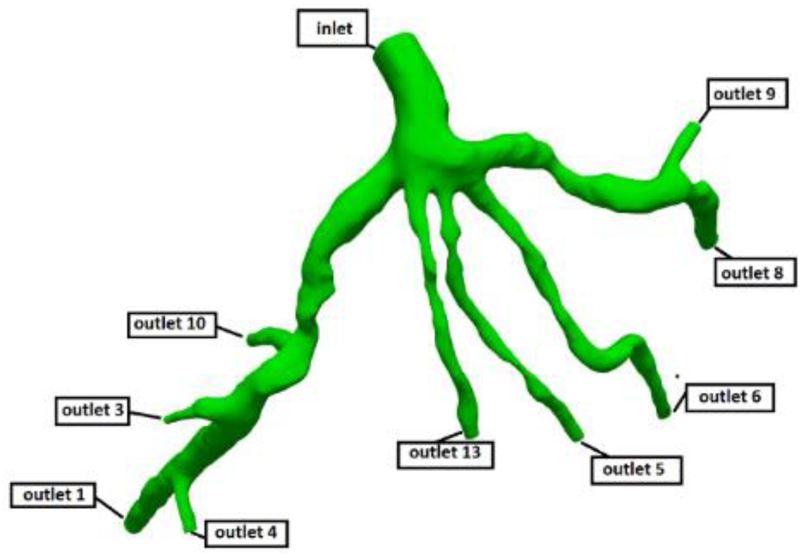
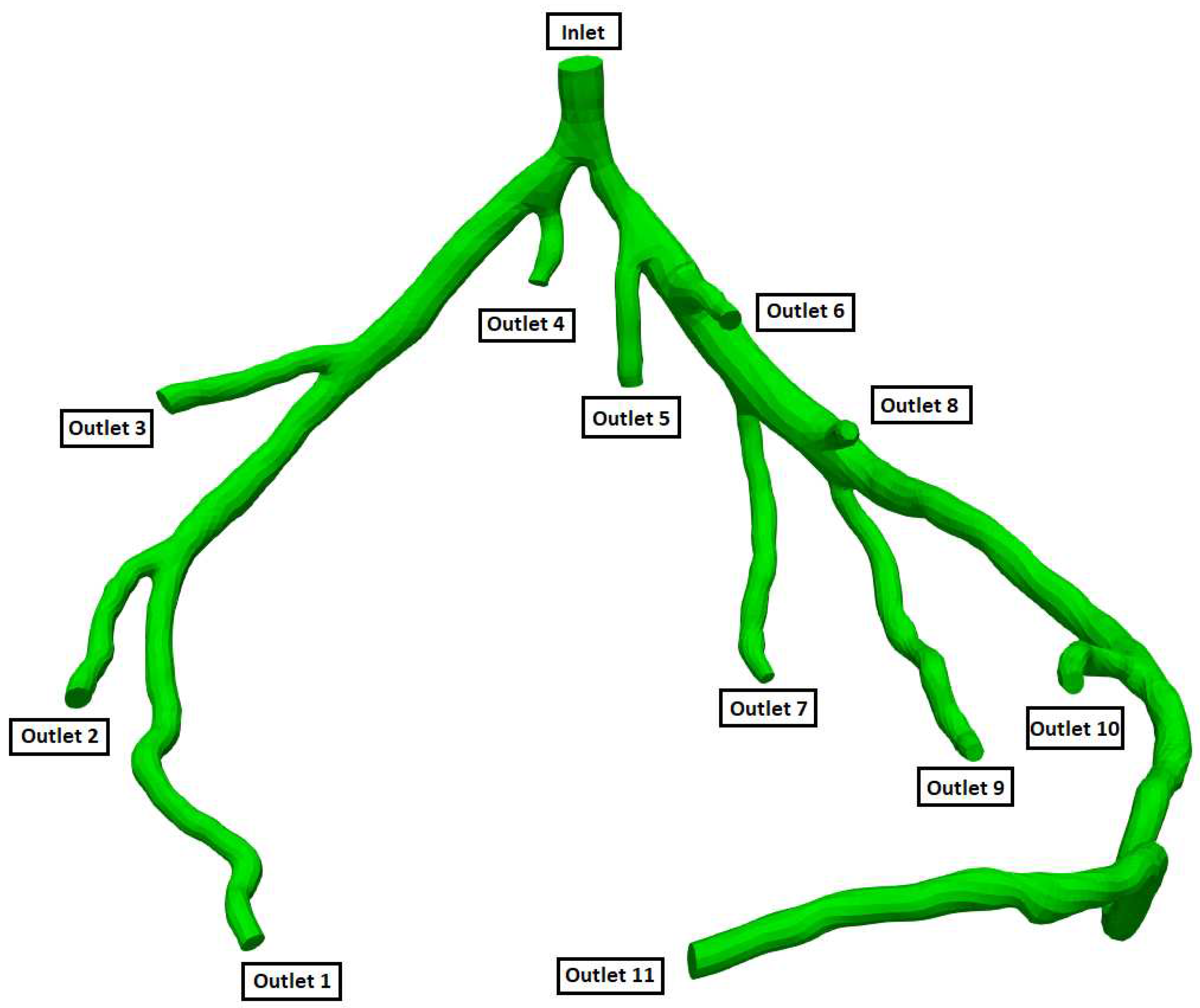
Estimated minimum mesh size for each mesh is about a half of the radius of the smallest artery (inlet/outlet) present in the model. Estimated mesh size for the coronary artery tree model CT209 (as shown in
Figure 3) is 0.1702, and for CHN13 it is 0.2262.
Table 10 and
Table 11 show the statistics of generated meshes. Mesh refinement has resulted in a larger number of mesh elements without the expansion layers near the vessel walls, which are difficult to implement due to the complexity of the geometries, which in turn increase the computational time for each simulation. For example, a decrease of mesh size from 0.20 to 0.1702 has resulted in 1.7 times increase in computational time.
The convergence criteria of for inlet pressure, defined in equation (12), is used for all computations.
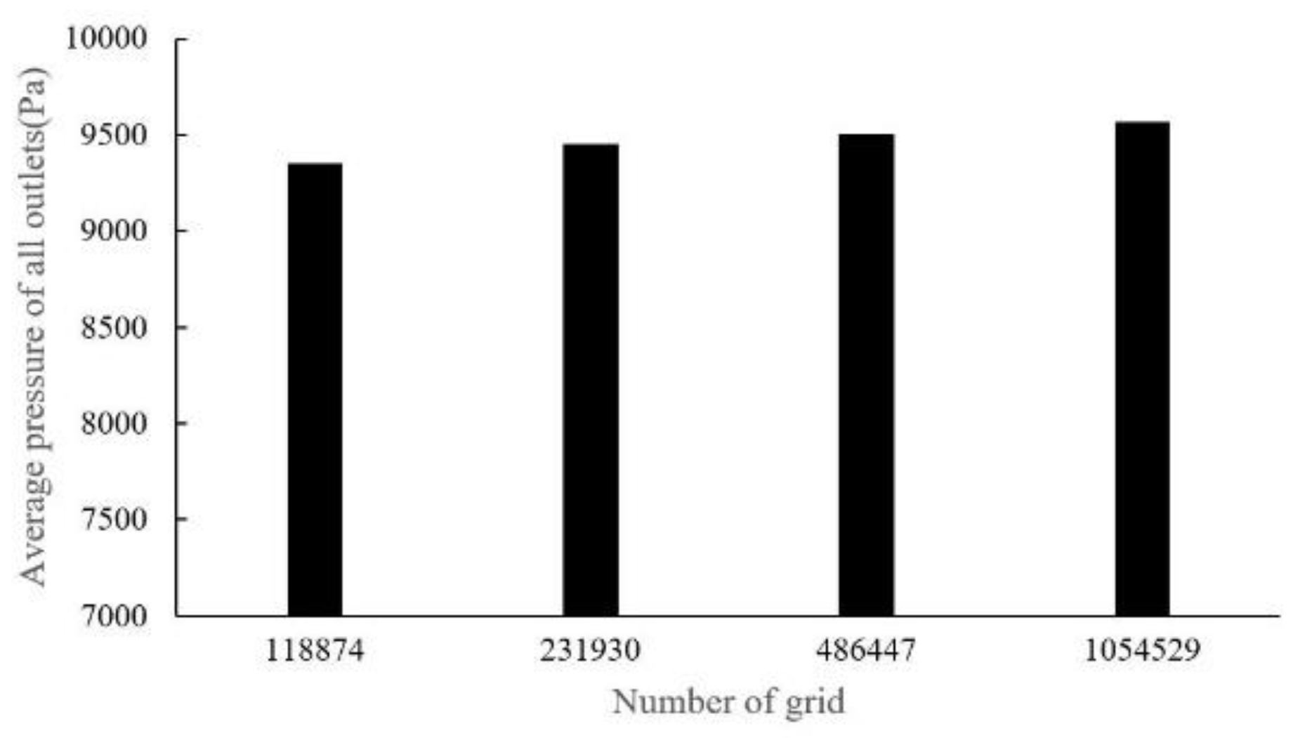
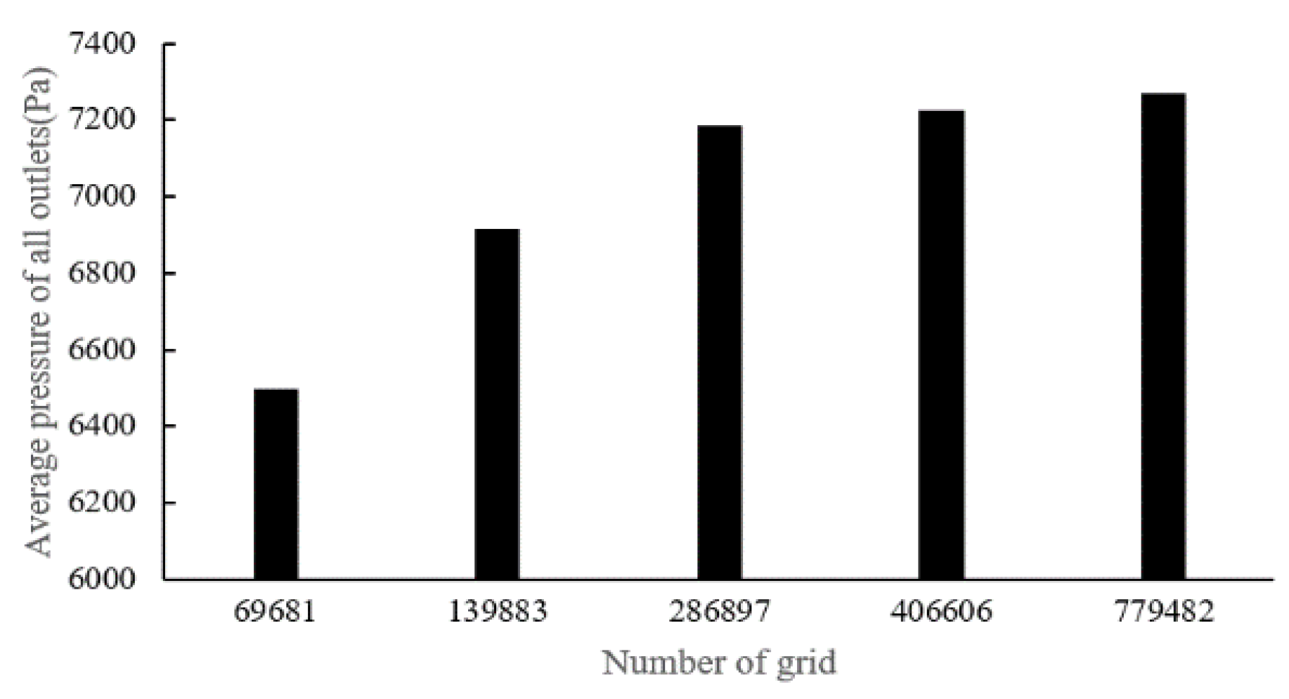
There are four sets of meshes generated for CT14 (with mesh cell numbers as: 118,874, 231,930, 486,447, 1,052,529) and five sets of meshes for CHN03 (with mesh element numbers as: 69,681, 139,833, 286,897, 406,606, 779,482) to study mesh convergence. The results are shown in
Figure 7 and
Figure 8.
Figure 7 shows that when the grid number is increased from 100,000 to about 1.05 million, the change value of the distal pressure is less than 5% (about 2.2%). After mesh dependency test, the model was discretized with a total of about 0.5 million volume cells. Further grid refinement leads to < 1% relative error. For case CHN03, the mesh convergent results are shown in
Figure 8. The number of volume cells was set to 0.4 million at last.
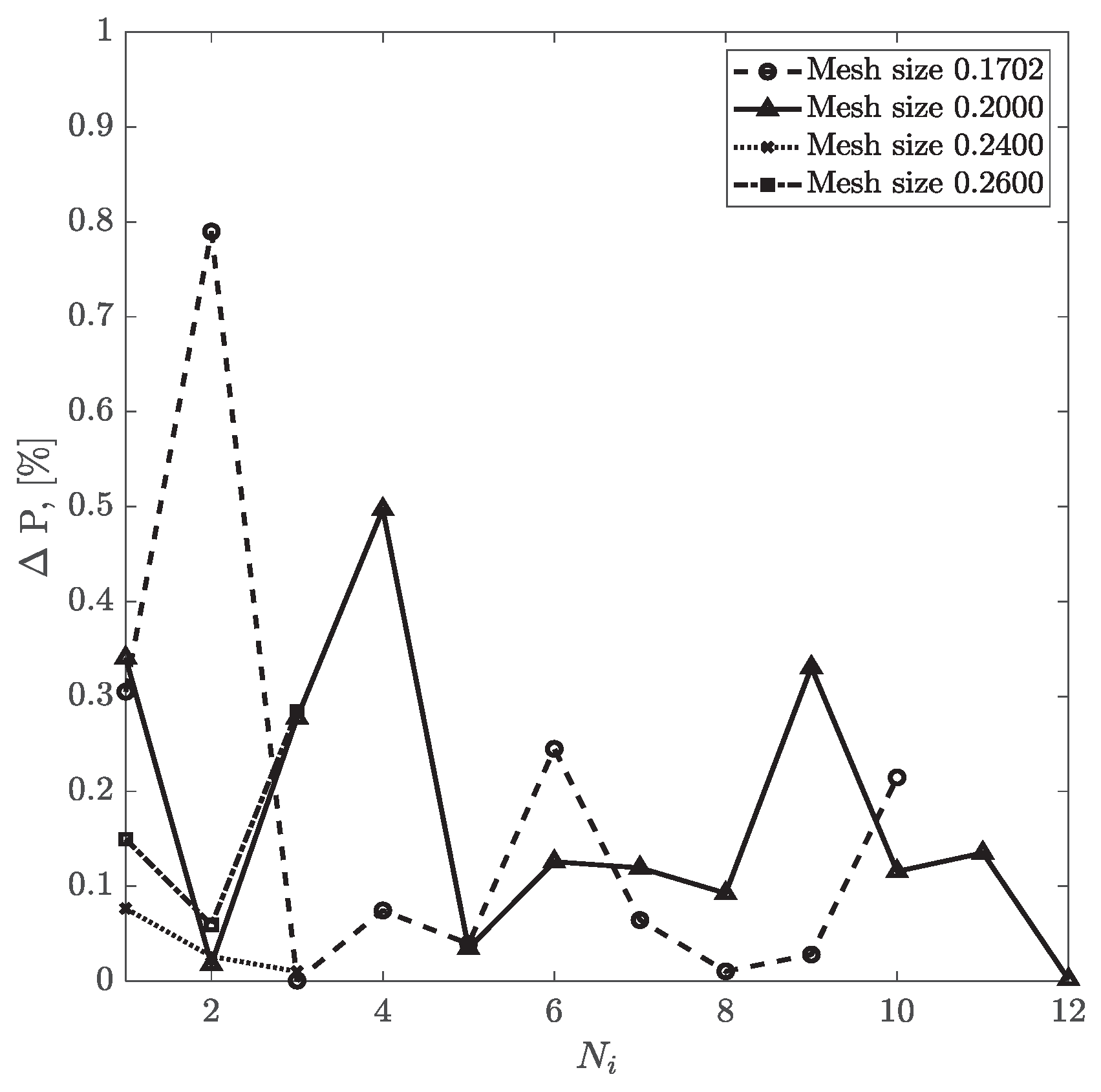
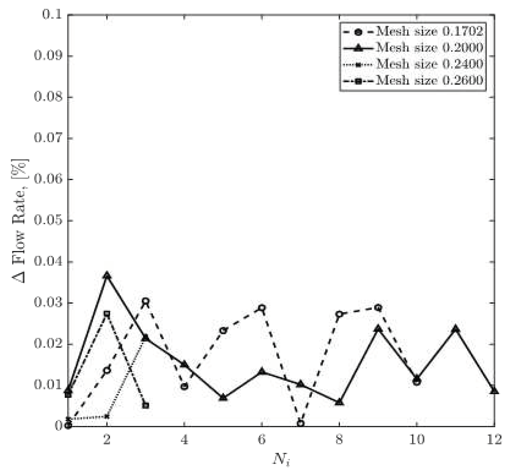
For CT209, the relative difference between experimental and computed values of inlet pressure and inlet flow values are plotted in
Figure 9 and
Figure 10, respectively. The relative percentage differences of calculated and experimentally measured (ICA) pressure and flow rate are obtained using equations (13) and (14). The overall trend shows that with more iterations, the relative difference values for pressure and flow rate decrease steadily for all four mesh sizes. Relative flow rate difference appears to be less than 0.04% for all iterations. The relative difference value for pressure for the mesh size of 0.1702 has dropped from 0.79% in the second iteration to 0.21% in the tenth iteration. However, for the mesh size of 0.20, relative pressure difference has decreased from 0.5% in the fourth round of iteration to 0.001% in the twelfth iteration.
Pressure and velocity residuals at all the outlets are defined as the averages of relative percentage differences in consecutive iterations. The convergence of CFD simulation can be monitored by examining the reduction of the values of the pressure and flow rate residuals at the outlets as well.
Figure 11 and
Figure 12 show pressure and flow rate residuals at the outlets for CT209, respectively, for all iterations where residual values are plotted in logarithmic scale. Mesh sizes of 0.1702 and 0.20 have the same fluctuation behaviors for all round of iterations. Minimum pressure residual values of 1.93E-7 and 2E-7 are observed for both meshes, whereas the maximum values are 3.62E-7 and 4.43E-7 respectively. It is important to note, that the mesh sizes of 0.24 and 0.26 show a different trend of fluctuations. The values of pressure residual fluctuate from 1.30 E-7 to 3.03E-7 in each consecutive simulation, i.e., in each round of iteration. In addition, greater magnitudes of residual fluctuations are observed in
Figure 11 and
Figure 12 for the mesh sizes of 0.24 and 0.26. For example, flow rate residual of 6.75E-6 is observed in the first iteration and it increases up to 2.72E-4 in the second one. However, finer meshes with the mesh sizes of 0.20 and 0.1702 do not show such an increase in flow rate residuals for each consecutive iteration.
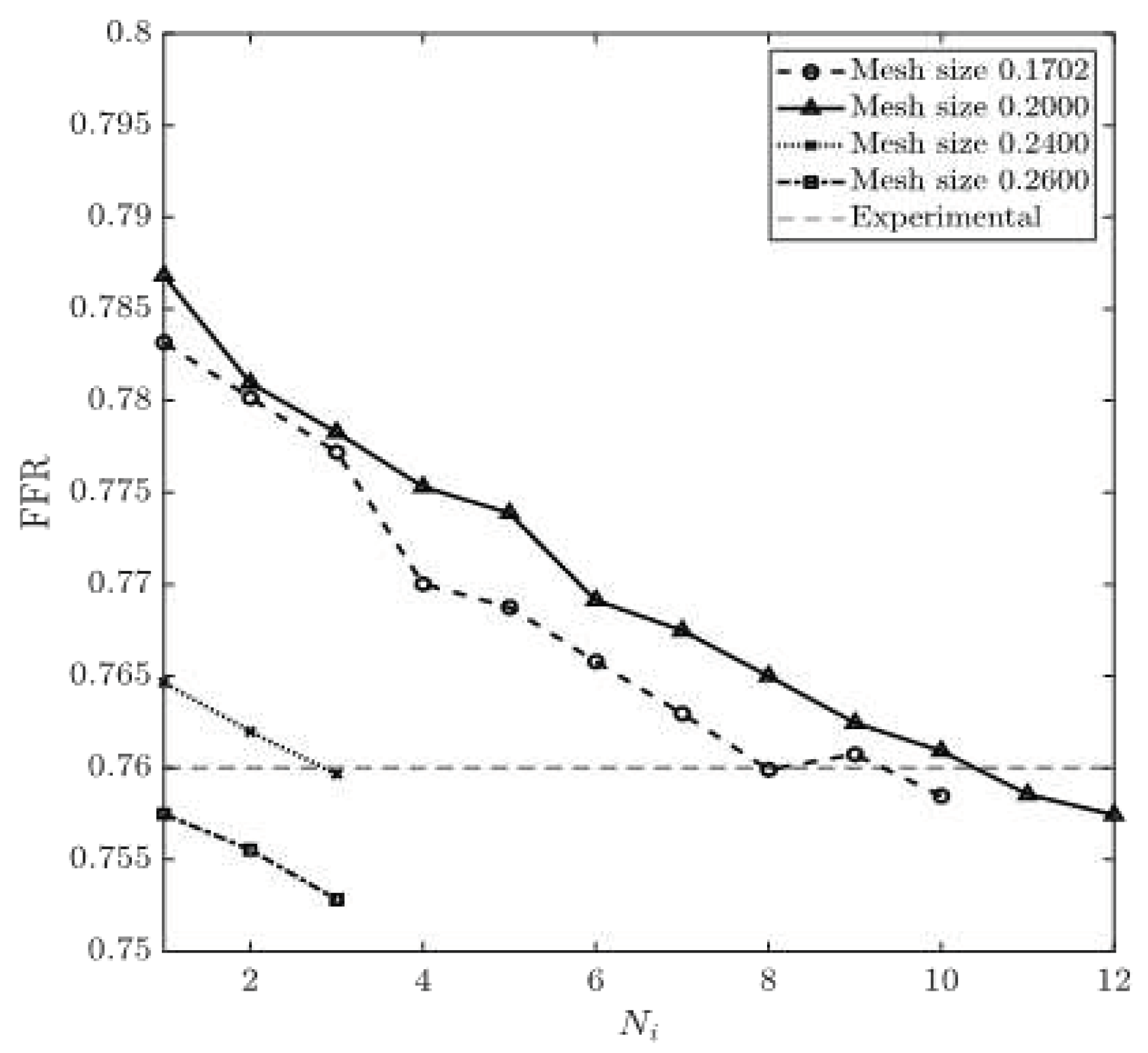
FFR is calculated using equation (15). The experimental value of FFR is 0.76 for CT209 model [16].
Figure 13 and
Figure 14 show the obtained values of FFR at each round of iteration and the percentage relative difference of calculated and experimental FFR (degree of deviation from experimentally obtained FFR). The results obtained from 0.1702 and 0.20 mesh sizes are very close to the experimental value of FFR=0.76 at the end of the eighth and the tenth round of iteration, respectively. At the same time, the results obtained from 0.24 and 0.26 mesh sizes demonstrate a constant decrease in
Figure 13, which yield a constant negative slope. FFR values for mesh sizes of 0.1702 and 0.20 have converged when they have reached the experimental FFR value. The percentage relative difference of FFR values of 0.20% and 0.34% are recorded for the mesh sizes of 0.1702 and 0.20, respectively. Zhang et al. [17] have computed non-invasive FFR value of 0.73 whereas experimental (ICA) FFR is about 0.76 for CT209 model. The final values of FFR for mesh sizes of 0.1702 and 0.20 are FFR=0.758 and FFR=0.757 which agree very well with the ICA FRR.
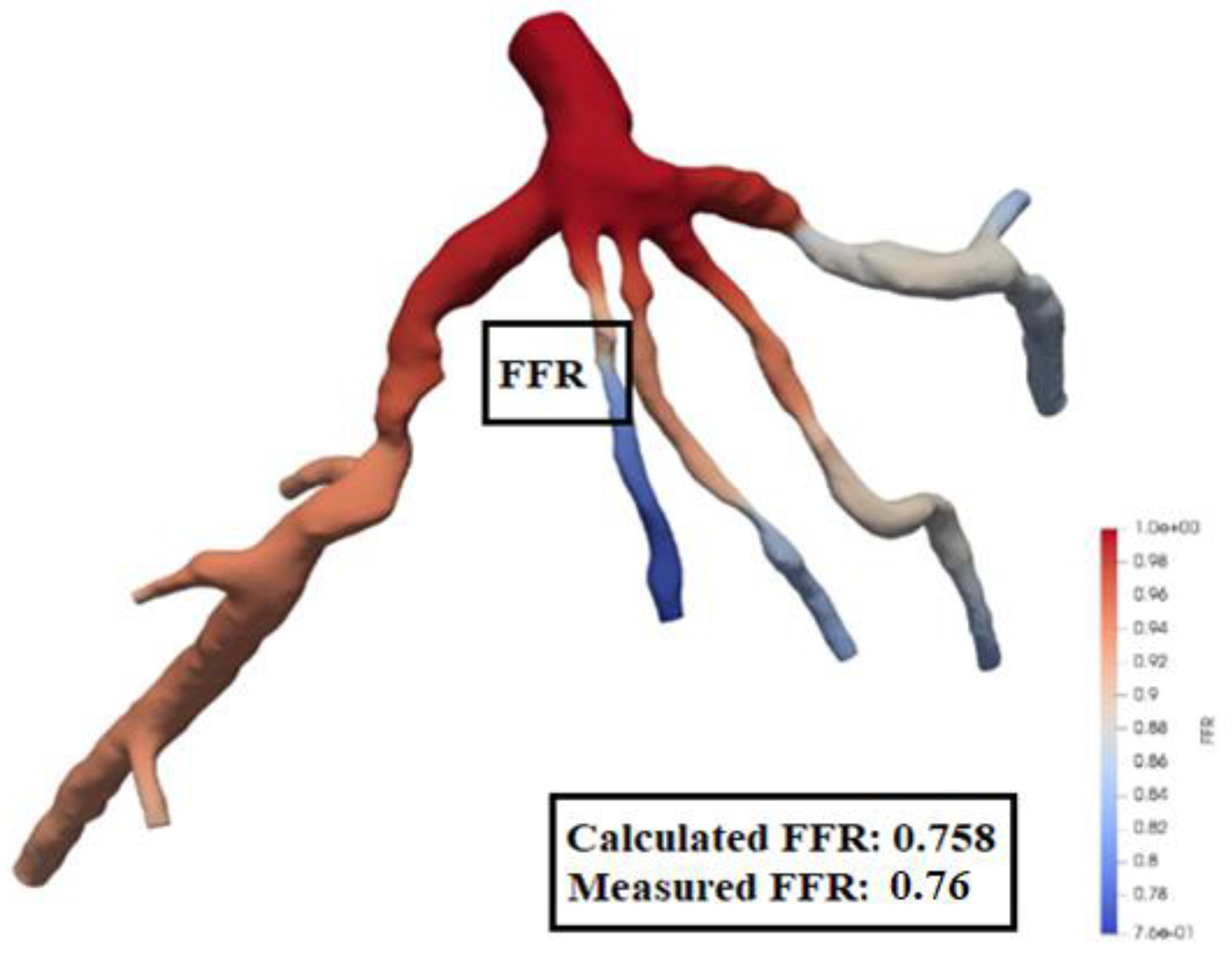
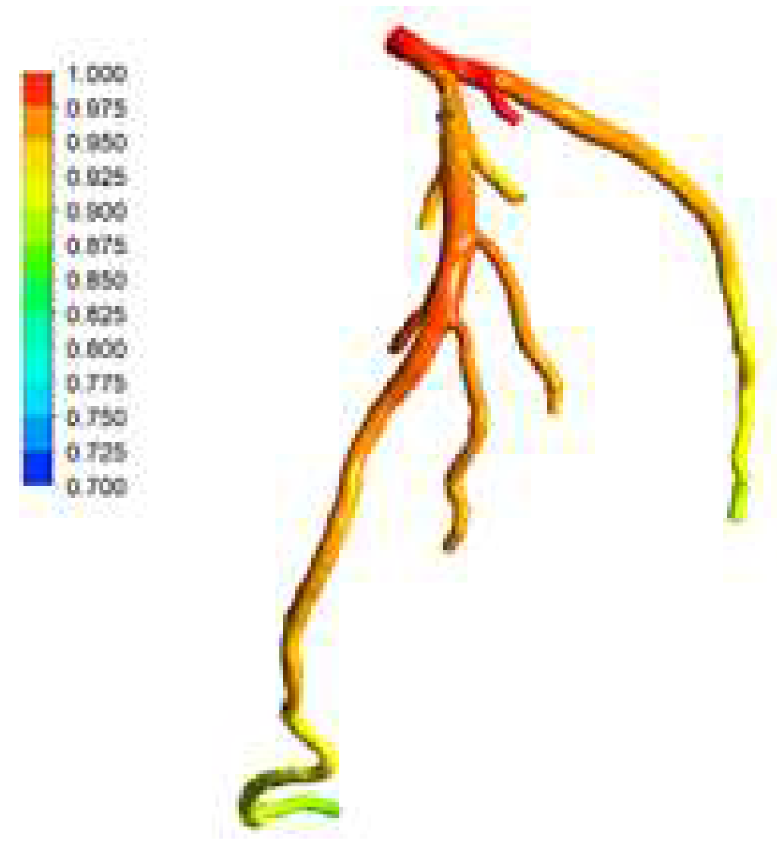
The location of Left Anterior Descending (LAD) Proximal artery is indicated as artery stenosis region for CT209 model in Zhang et al. [17]. The dark blue region of the blood vessel is LAD Proximal in
Figure 15. Therefore, it is found that the artery stenosis is located in the same region as it was observed by Zhang et al. [17].
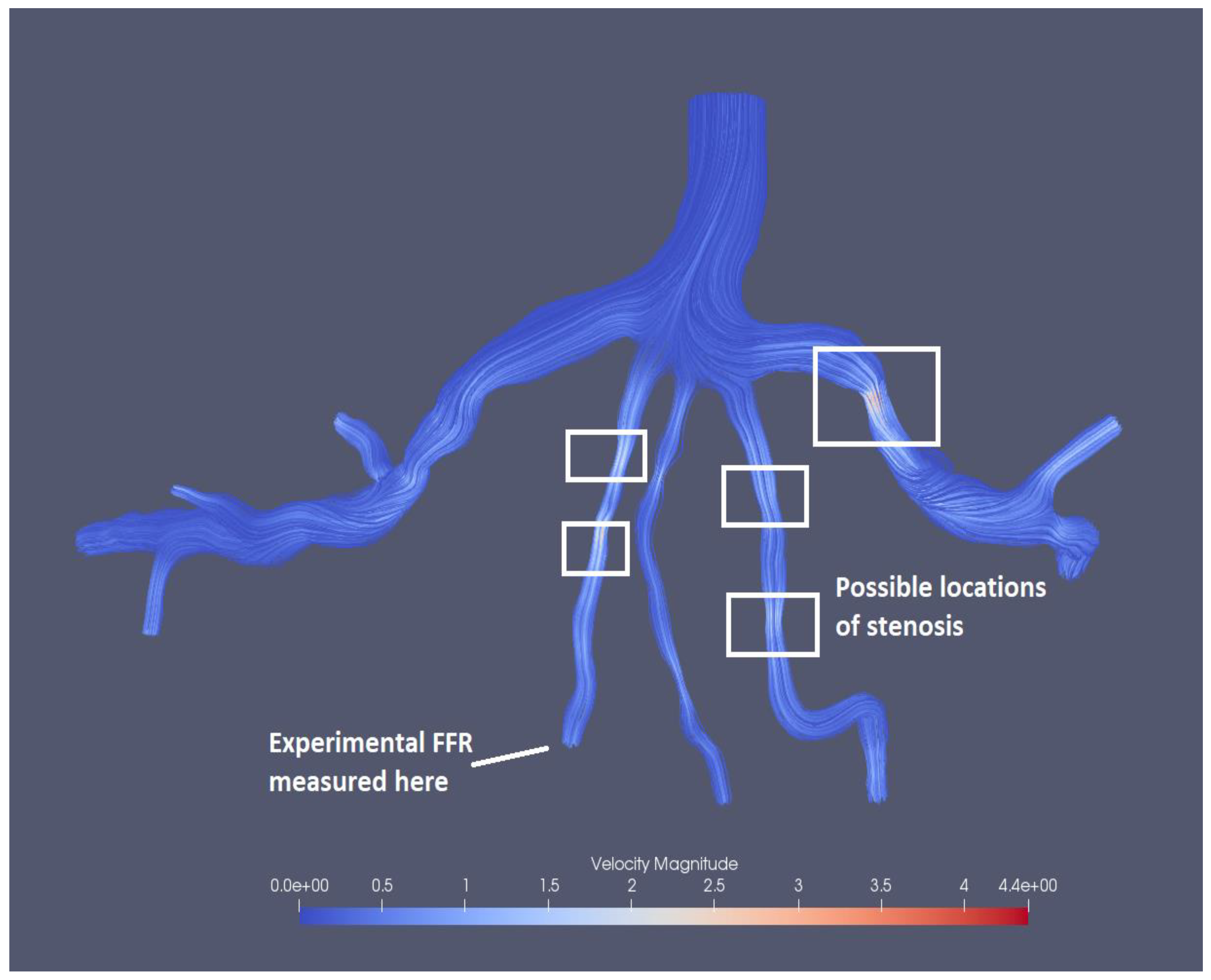
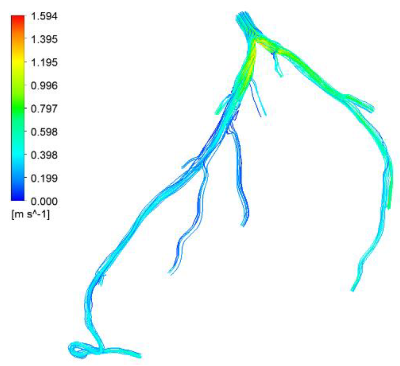
Figure 15 presents the visualized results of FFR at the end of the tenth iteration for the mesh size of 0.1702. The visualization of velocity streamlines is presented in
Figure 16, where it can be observed that there is an increase in velocity magnitude in the stenotic region and several possible stenosis are also identified in the figure based on velocity magnitudes.
The simulations of blood flow in the model CHN13 are performed using three mesh sizes (coarse, fine and very fine). Initially, the number of iterations is set to ten, however, since the relative errors for some mesh sizes show systematic increases, the simulations with 0.53 and 0.22 mesh sizes are stopped at the fifth and sixth rounds of iterations, respectively. The relative inlet pressure differences from the corresponding measurements calculated for the three meshes demonstrate that the maximum pressure difference is less than 1% for all cases, and at the same time, the relative inlet pressure difference is minimum for the mesh size of 0.22 as shown in
Figure 17. The relative differences of inlet flow rates for all three mesh sizes are less than 1% with a maximum of 0.02% observed for the finest mesh (see
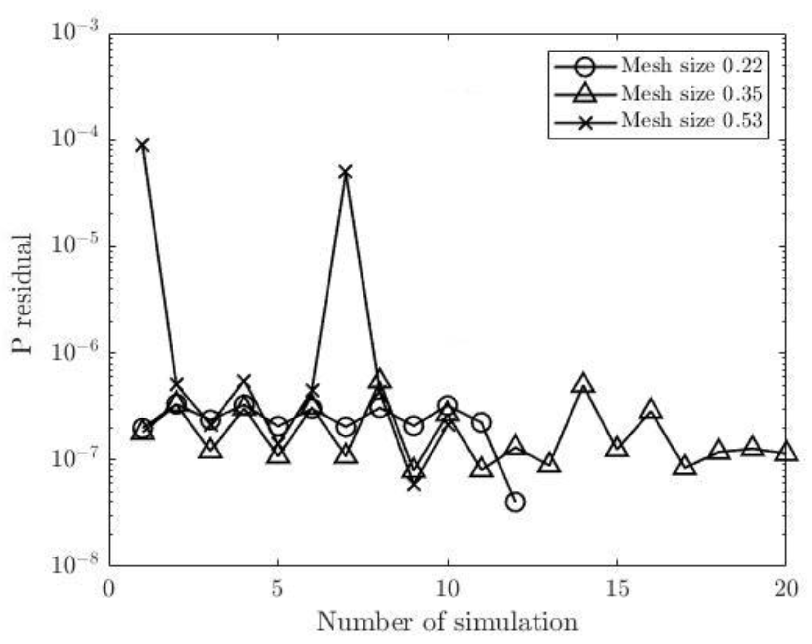
Figure 18). The pressure and flow rate residuals at the outlets for CHN13 are shown in
Figure 19 and
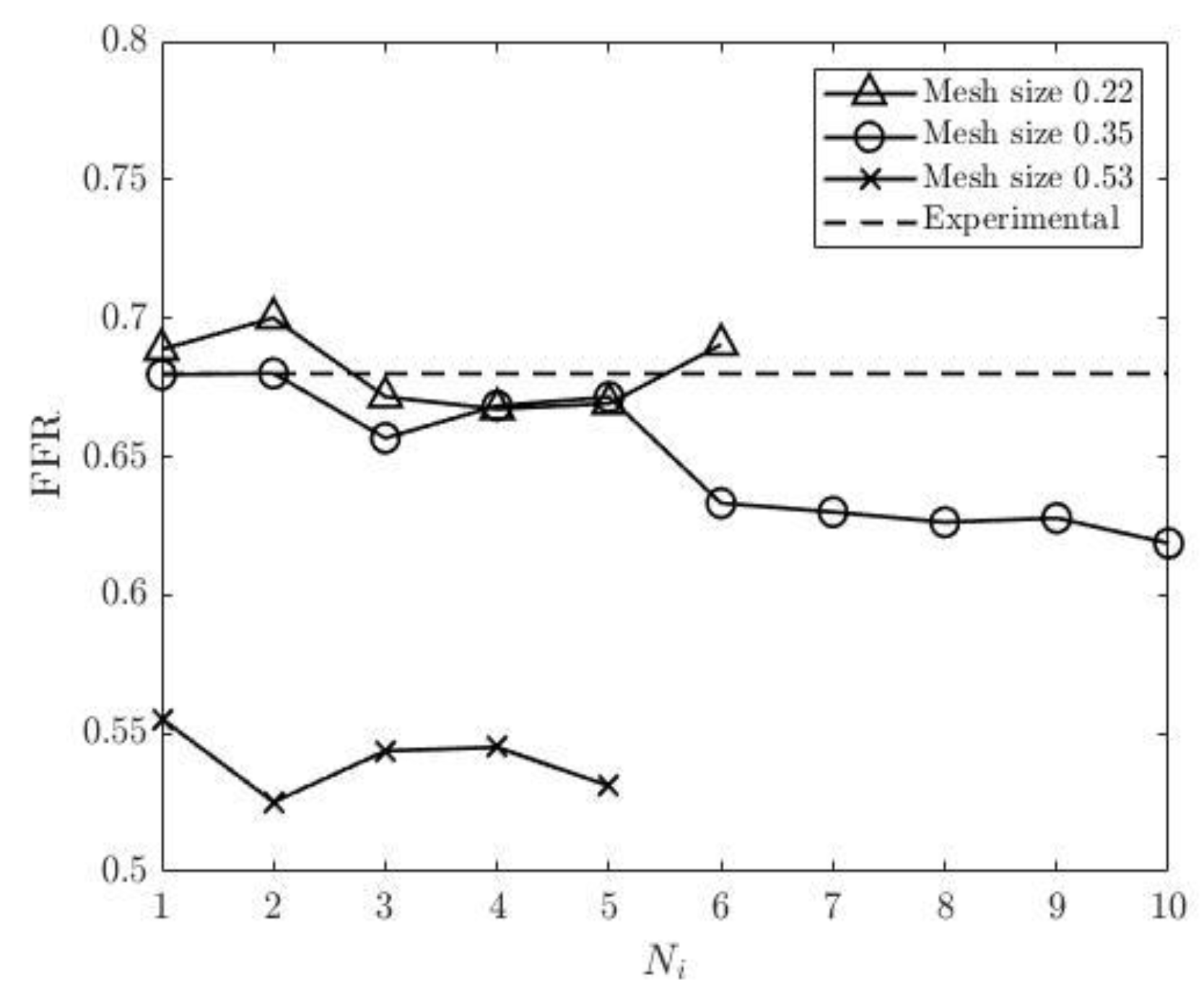
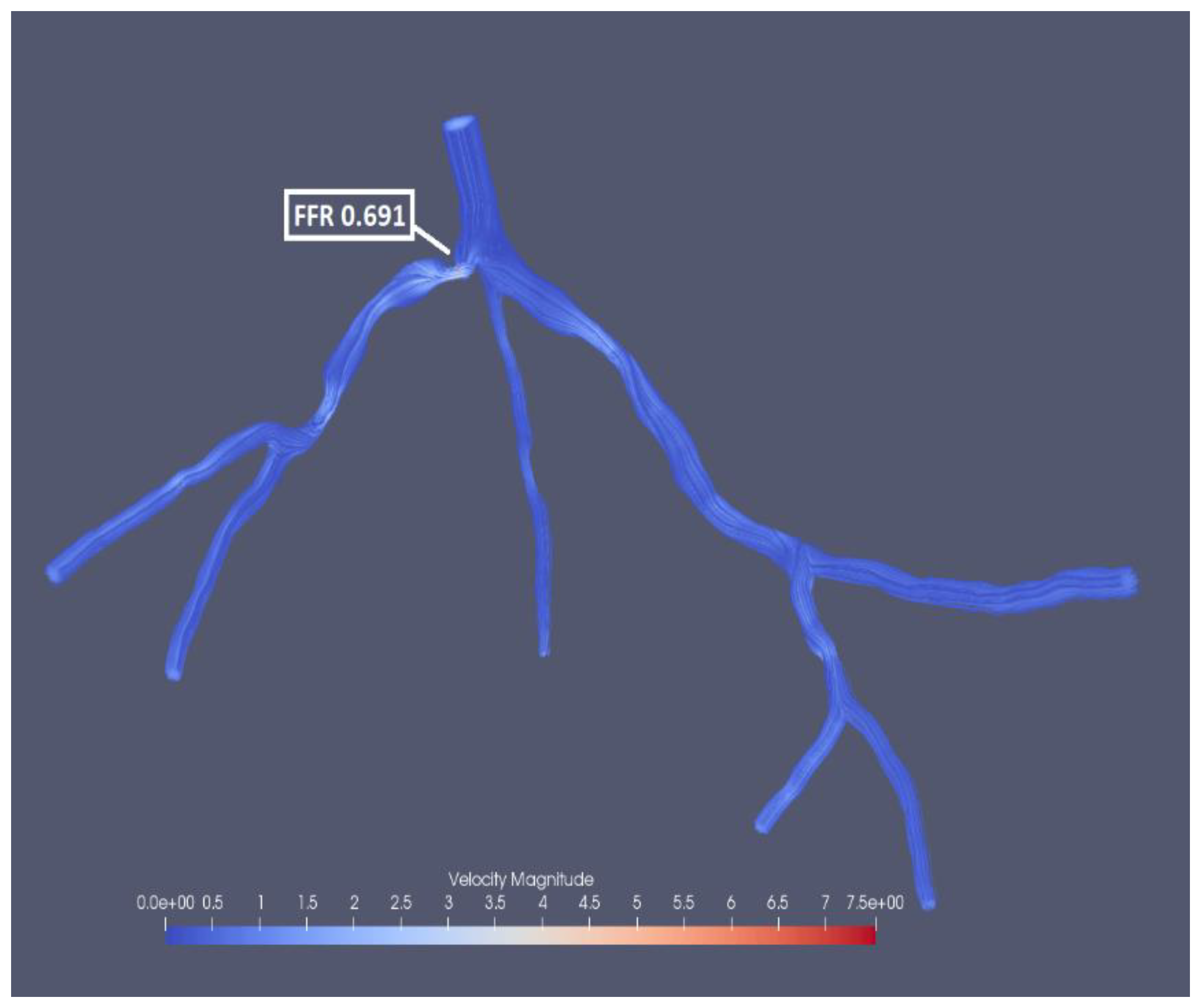
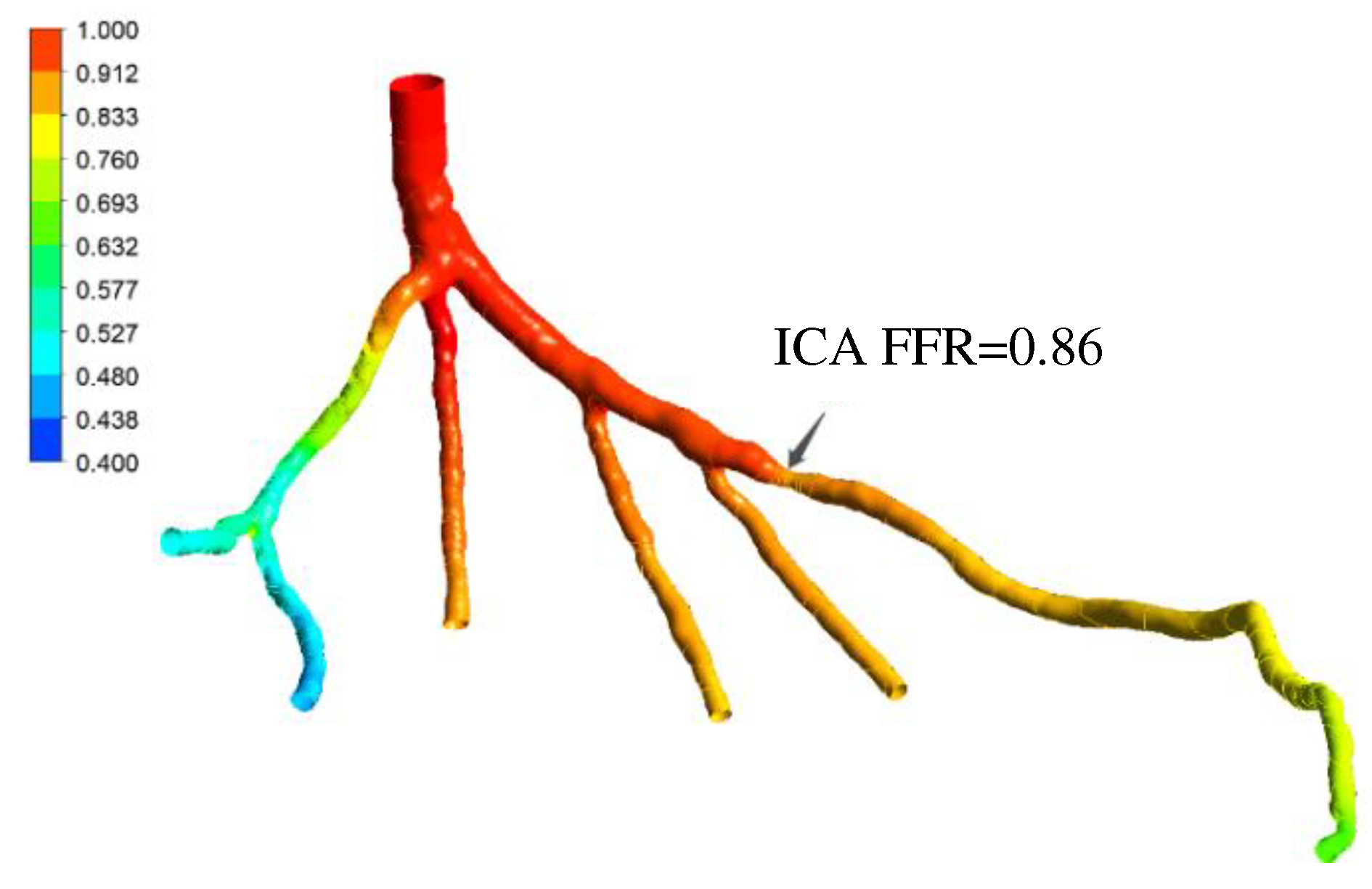
Figure 20, which fluctuate for all three mesh sizes. The most significant fluctuation is observed for pressure residual with the mesh size of 0.53 (from 5.91*10-8 to 8.95*10-5) and for flow rate residual with 0.35 in mesh size (from 1.7*10-6 to 1.71*10-4). Interestingly the finest mesh size has relatively low pressure residuals (in the interval from 4.02*10-8 to 3.32*10-7) and high flow rate residuals (from 2.33*10-5 to 2.03*10-4). The experimental FFR for the CHN13 model is 0.68. The results show that the finest mesh size (0.22) produces the closest to this value. FFR obtained from the simulations with the finest mesh size is equal to 0.691 as shown in
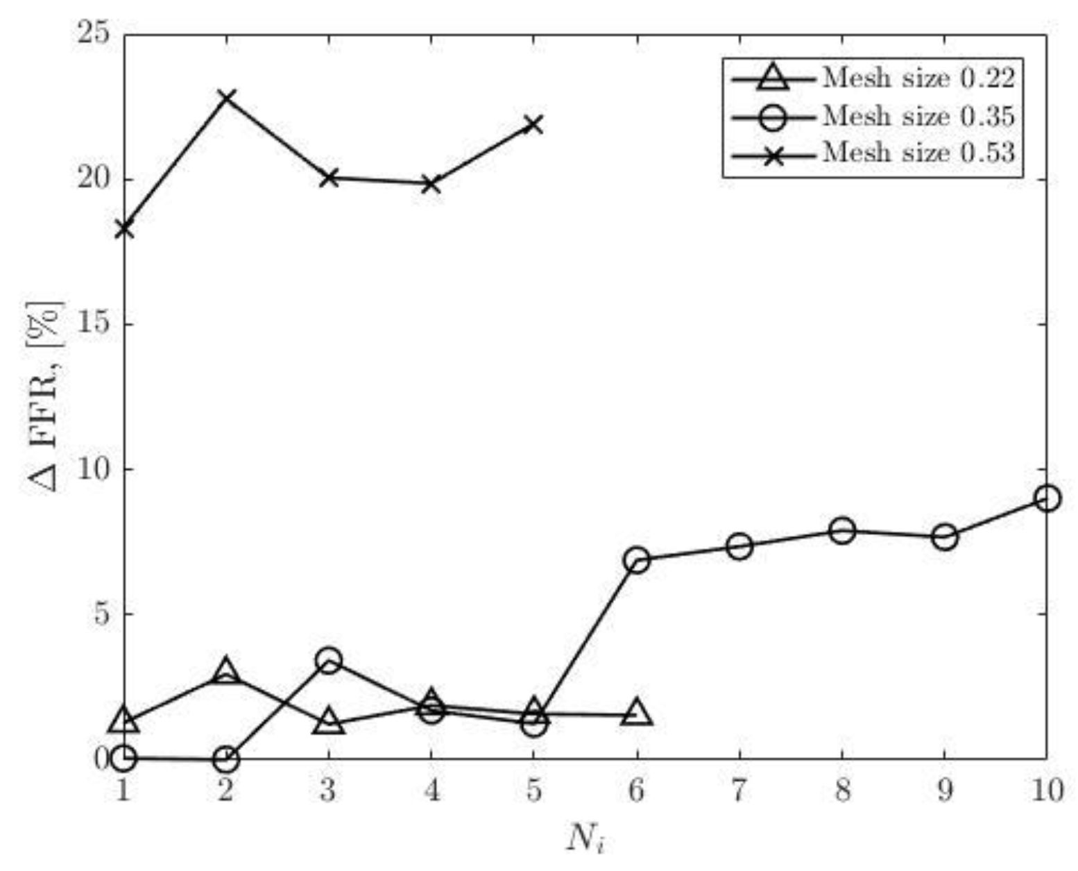
Figure 21. The final values of FFR obtained using 0.35 and 0.53 mesh sizes are 0.619 and 0.531, respectively. Additionally, the results in
Figure 22 show that the accuracy of the FFR obtained from simulations with 0.35 in mesh size decreases with the number of iterations. Consequently, the maximum error is observed in the tenth round of iterations.
Figure 23 shows a significant decrease in FFR at the location of stenosis caused by pressure drop. The velocity streamlines are presented in
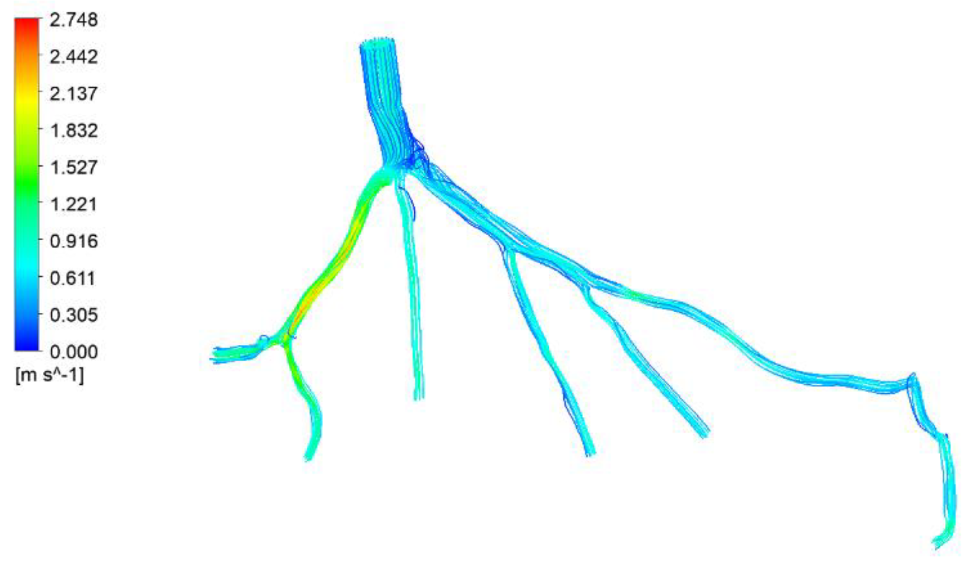
Figure 24. The color of the streamlines at the stenosis indicates an increase in velocity.
Figure 25 shows the comparison between the results obtained by traditional lumped parameter method and those obtained by the current method as well as the ICA measurement. It is found that the current method demonstrates better accuracy and efficiency than the traditional methods.
Figure 26 and
Figure 27 present the visualized pressure distributions for the models CT14 and CHN03, respectively. The calculated FFRs for CT14 and CHN03 by the PBA are 0,975 and 0.691 as shown in
Figure 21,
Figure 22,
Figure 23,
Figure 24,
Figure 25,
Figure 26 and
Figure 27, which have excellent agreement with the corresponding experimental values of 0.97 and 0. 68 respectively. The visualizations of velocity streamlines are represented in
Figure 28 and
Figure 29.
Finally a summary of the comparison of the calculated and experimental ICA FFRs are presented in the
Table 12. The results show that the differences between the relative errors for Ansys and Simvascular is at most of 3.24%. This shows that the proposed PBA produces results that are solver independent.
Further validation of the PBA method is performed using traditional LPM method described in the paper by Zhang et al [17] for model CT14. The LPM method uses a reference pressure, resistances at every outlet representing the flow resistance from the downstream microvasculature, an overall resistance for the whole CAT which is related to the outlet resistances through an population-averaged empirical scaling law [17], and an iterative procedure to calculate the resistances and reference pressure, thus resulting in the outlet pressures in each branch outlet. Three simulations were run for the model CT14 using both methods: the traditional LPM method is run using Ansys, while the proposed PBA is used in Simvascular.
Table 13 compares the flow rates at the outlets, which show that the percentage deviations between the flow rates obtained using PBA and LPM are below 0.1%, yielding on average 0.036%.
It is found that the LPM cannot always guarantee convergence to a unique solution for every case, while the proposed PBA can generate convergence to accurate solutions for all the four cases studied. This shows that the PBA is far more robust than the LPM because the former is physiologically based and patient specific while the latter is not!
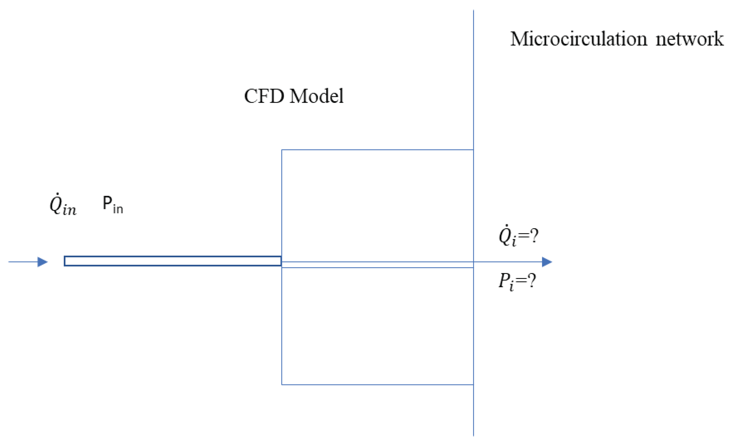
Figure 1.
Schematic of the new boundary model.
Figure 1.
Schematic of the new boundary model.
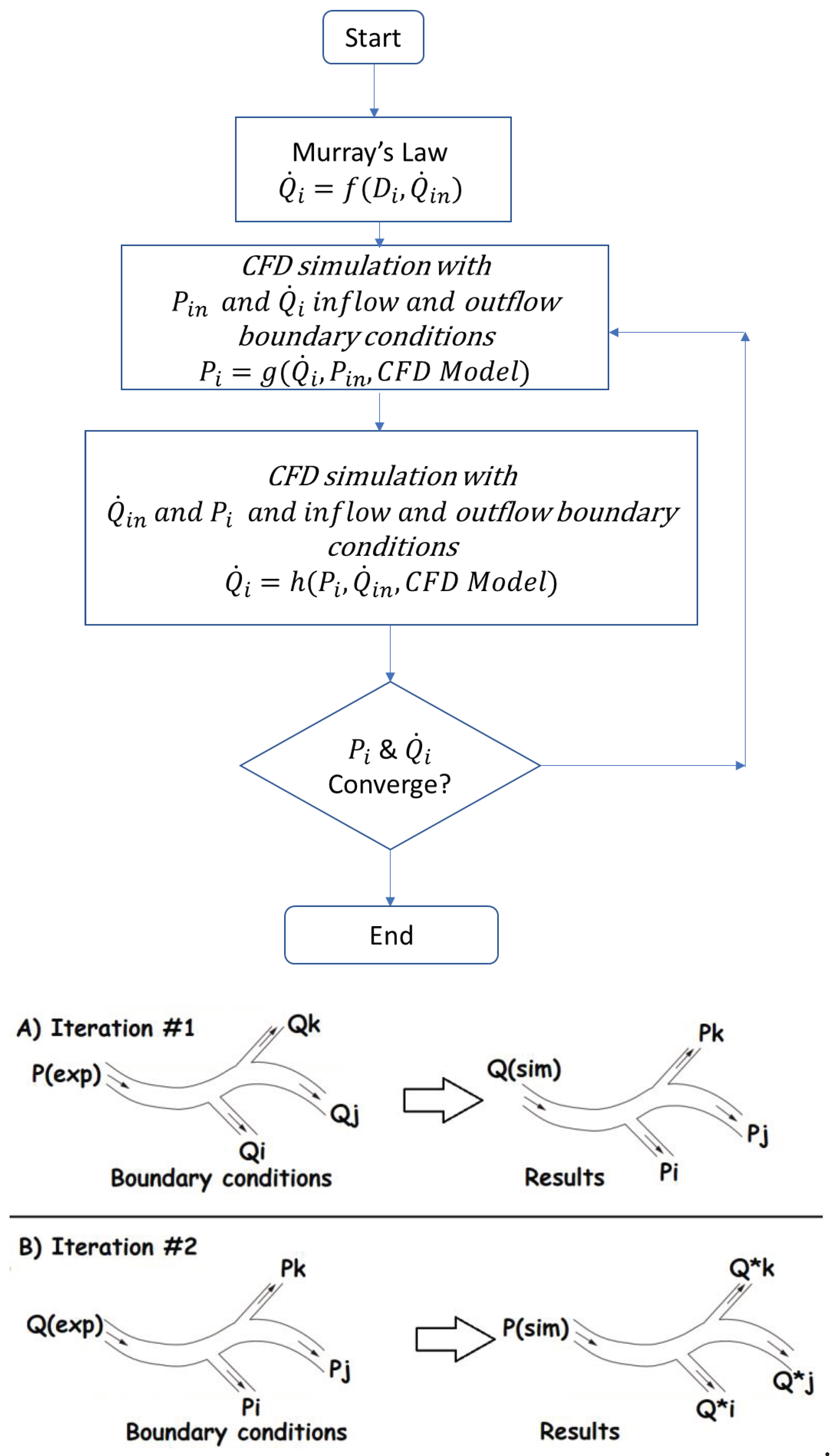
Figure 2.
Algorithm for the outflow boundary conditions.
Figure 2.
Algorithm for the outflow boundary conditions.
Figure 3.
Geometry and Outlets of the CT209 model.
Figure 3.
Geometry and Outlets of the CT209 model.
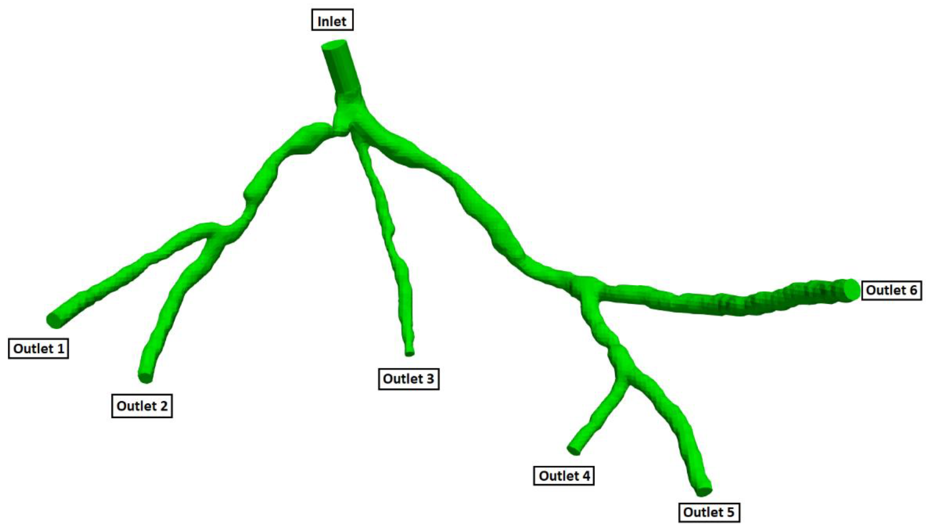
Figure 4.
Geometry and Outlets of the CHN13 model.
Figure 4.
Geometry and Outlets of the CHN13 model.
Figure 5.
Geometry and Outlets of the CT14 model.
Figure 5.
Geometry and Outlets of the CT14 model.
Figure 6.
Geometry and Outlets of the CHN03 model.
Figure 6.
Geometry and Outlets of the CHN03 model.
Figure 7.
Dependency analysis for CT14.
Figure 7.
Dependency analysis for CT14.
Figure 8.
Dependency analysis for CHN03.
Figure 8.
Dependency analysis for CHN03.
Figure 9.
Inlet pressure relative percentage deviation from the experimental value vs No. of iterations for CT209.
Figure 9.
Inlet pressure relative percentage deviation from the experimental value vs No. of iterations for CT209.
Figure 10.
Inlet flow rate relative percentage deviation from the experimental value vs No. of iterations for CT209.
Figure 10.
Inlet flow rate relative percentage deviation from the experimental value vs No. of iterations for CT209.
Figure 11.
Outlet pressure residual vs No. of iterations for CT209.
Figure 11.
Outlet pressure residual vs No. of iterations for CT209.
Figure 12.
Outlet flow rate residual vs No. of iterations for CT209.
Figure 12.
Outlet flow rate residual vs No. of iterations for CT209.
Figure 13.
FFR values in each round of iteration for CT209.
Figure 13.
FFR values in each round of iteration for CT209.
Figure 14.
Relative differences between calculated and experimental FFR in each round of iteration for CT209.
Figure 14.
Relative differences between calculated and experimental FFR in each round of iteration for CT209.
Figure 15.
FFR distribution along with the shape of CT209 model.
Figure 15.
FFR distribution along with the shape of CT209 model.
Figure 16.
Visualization of velocity streamlines in the CT 209 model.
Figure 16.
Visualization of velocity streamlines in the CT 209 model.
Figure 17.
Inlet pressure relative percentage deviation from the experimental value vs No. of iterations for CHN13
Figure 17.
Inlet pressure relative percentage deviation from the experimental value vs No. of iterations for CHN13
Figure 18.
Inlet flow rate relative percentage deviation from the experimental value vs No. of iterations for CHN13.
Figure 18.
Inlet flow rate relative percentage deviation from the experimental value vs No. of iterations for CHN13.
Figure 19.
Outlet pressure residual vs No. of iterations for CHN13.
Figure 19.
Outlet pressure residual vs No. of iterations for CHN13.
Figure 20.
Outlet flow rate residual vs No. of iterations for CHN13.
Figure 20.
Outlet flow rate residual vs No. of iterations for CHN13.
Figure 21.
FFR values in each round of iteration for CHN13.
Figure 21.
FFR values in each round of iteration for CHN13.
Figure 22.
Relative differences between calculated and experimental FFR in each round of iteration for CHN13.
Figure 22.
Relative differences between calculated and experimental FFR in each round of iteration for CHN13.
Figure 23.
FFR distribution along with the shape of CHN13 model.
Figure 23.
FFR distribution along with the shape of CHN13 model.
Figure 24.
Visualization of velocity streamlines in the CHN13 model.
Figure 24.
Visualization of velocity streamlines in the CHN13 model.
Figure 25.
Validation of FFR obtained using PBA with CT14: A) 3D Model of a coronary artery tree; B) FFR obtained from traditional lumped parameter method; C) FFR obtained from ICA; D) FFR obtained using the proposed PBA.
Figure 25.
Validation of FFR obtained using PBA with CT14: A) 3D Model of a coronary artery tree; B) FFR obtained from traditional lumped parameter method; C) FFR obtained from ICA; D) FFR obtained using the proposed PBA.
Figure 26.
Pressure distributions on CT14
Figure 26.
Pressure distributions on CT14
Figure 27.
Pressure distributions on CHN03
Figure 27.
Pressure distributions on CHN03
Figure 28.
Visualization of velocity streamlines in CHN03
Figure 28.
Visualization of velocity streamlines in CHN03
Figure 29.
Visualization of velocity streamlines in CT14
Figure 29.
Visualization of velocity streamlines in CT14
Table 1.
Workflow procedure of Rapid Iterative algorithm.
Table 1.
Workflow procedure of Rapid Iterative algorithm.
| |
|
Inlet |
Outlets |
| 1st round of iteration |
Input to CFD Solver |
a
|
|
|
… |
|
|
*calculated by Murray’s law at beginning
|
| The output from CFD Solver |
|
|
|
… |
|
| Input to CFD solver |
b
|
|
|
… |
|
| Output from CFD Solver |
|
|
|
… |
|
| 2nd round of iteration |
Input to CFD solver |
|
|
|
… |
|
| Output from CFD solver |
|
|
|
… |
|
| Input to CFD solver |
|
|
|
… |
|
| Output from CFD solver |
|
|
|
… |
|
| Nth round of iteration |
- |
- |
- |
- |
- |
- |
Table 2.
Experimentally obtained input parameters for simulation for CT209.
Table 2.
Experimentally obtained input parameters for simulation for CT209.
| Parameter |
Value |
|
90.53 mm Hg (12070.12 Pa) |
| Experimental inlet flow rate |
9.39944 cm3/s |
Table 3.
Experimentally obtained input parameters for simulation for CHN13.
Table 3.
Experimentally obtained input parameters for simulation for CHN13.
| Parameter |
Value |
|
90.61 mm Hg (12870.12 Pa) |
| Experimental inlet flow rate |
7.17551 cm3/s |
Table 4.
Experimentally obtained input parameters for simulation for CT14.
Table 4.
Experimentally obtained input parameters for simulation for CT14.
| Parameter |
Value |
|
76.8 mm Hg (10240.8 Pa) |
| Experimental inlet flow rate |
6.19 cm3/s |
Table 5.
Experimentally obtained input parameters for simulation for CHN03.
Table 5.
Experimentally obtained input parameters for simulation for CHN03.
| Parameter |
Value |
|
76.5 mm Hg (10201.9 Pa) |
| Experimental inlet flow rate |
6.18 cm3/s |
Table 6.
Initial calculated flow rates at each outlet by Murray's law for CT209.
Table 6.
Initial calculated flow rates at each outlet by Murray's law for CT209.
| Murray’s law calculation for outlet flow rates |
| |
|
(cm2) |
(cm) |
(cm3) |
|
(cm3/s) |
| outlet 1 |
1 |
4.114 |
2.289 |
11.988 |
0.315 |
2.965 |
| outlet 3 |
2 |
0.568 |
0.851 |
0.616 |
0.016 |
0.152 |
| outlet 4 |
3 |
0.925 |
1.085 |
1.279 |
0.034 |
0.316 |
| outlet 5 |
4 |
0.977 |
1.116 |
1.388 |
0.037 |
0.343 |
| outlet 6 |
5 |
1.802 |
1.515 |
3.475 |
0.091 |
0.859 |
| outlet 8 |
6 |
4.105 |
2.286 |
11.948 |
0.314 |
2.955 |
| outlet 9 |
7 |
1.674 |
1.460 |
3.111 |
0.082 |
0.769 |
| outlet 10 |
8 |
1.173 |
1.222 |
1.824 |
0.048 |
0.451 |
| outlet 13 |
9 |
1.398 |
1.334 |
2.374 |
0.062 |
0.587 |
Table 7.
Initial calculated flow rates at each outlet by Murray's law for CHN13.
Table 7.
Initial calculated flow rates at each outlet by Murray's law for CHN13.
| Murray’s law calculation for outlet flow rates |
|---|
| |
|
(cm2) |
(cm) |
(cm3) |
|
(cm3/s) |
| outlet 1 |
6 |
2.712 |
1.858 |
6.418 |
0.227 |
1.630 |
| outlet 2 |
1 |
1.832 |
1.527 |
3.564 |
0.126 |
0.905 |
| outlet 3 |
3 |
1.005 |
1.131 |
1.447 |
0.051 |
0.368 |
| outlet 4 |
2 |
1.950 |
1.576 |
3.913 |
0.139 |
0.994 |
| outlet 5 |
5 |
1.969 |
1.583 |
3.970 |
0.141 |
1.009 |
| outlet 6 |
4 |
3.382 |
2.075 |
8.936 |
0.316 |
2.270 |
Table 8.
Initial calculated flow rates at each outlet by Murray's law for CT14.
Table 8.
Initial calculated flow rates at each outlet by Murray's law for CT14.
| Murray’s law calculation for outlet flow rates |
| |
|
(cm2) |
(cm) |
(cm3) |
|
(cm3/s) |
| outlet 1 |
1 |
2.0253 |
1.6058 |
4.1410 |
0.1008 |
0.6238 |
| outlet 2 |
2 |
2.5091 |
1.7874 |
5.7102 |
0.1390 |
0.8602 |
| outlet 3 |
3 |
2.8210 |
1.8952 |
6.8072 |
0.1657 |
1.0254 |
| outlet 4 |
4 |
1.8029 |
1.5151 |
3.4779 |
0.0846 |
0.5239 |
| outlet 5 |
5 |
1.9039 |
1.5570 |
3.7744 |
0.0919 |
0.5686 |
| outlet 6 |
6 |
2.2769 |
1.7026 |
4.9359 |
0.1201 |
0.7436 |
| outlet 7 |
7 |
1.2534 |
1.2633 |
2.0160 |
0.0491 |
0.3037 |
| outlet 8 |
8 |
1.0056 |
1.1315 |
1.4487 |
0.0353 |
0.2182 |
| outlet 9 |
9 |
1.2546 |
1.2639 |
2.0189 |
0.0491 |
0.3041 |
| outlet 10 |
10 |
1.3891 |
1.3299 |
2.3522 |
0.0572 |
0.3543 |
| outlet 11 |
11 |
2.11181 |
1.6398 |
4.4091 |
0.1073 |
0.6642 |
Table 9.
Initial calculated flow rates at each outlet by Murray's law for CHN03.
Table 9.
Initial calculated flow rates at each outlet by Murray's law for CHN03.
| Murray’s law calculation for outlet flow rates |
| |
|
(cm2) |
(cm) |
(cm3) |
|
(cm3/s) |
| outlet 1 |
1 |
2.5675 |
1.8081 |
5.9106 |
0.2240 |
1.3847 |
| outlet 2 |
2 |
2.2262 |
1.6836 |
4.7721 |
0.1808 |
1.1179 |
| outlet 3 |
3 |
2.1930 |
1.6710 |
4.6658 |
0.1768 |
1.0930 |
| outlet 4 |
4 |
1.8206 |
1.5225 |
3.5293 |
0.1338 |
0.8268 |
| outlet 5 |
5 |
1.7784 |
1.5048 |
3.4074 |
0.1291 |
0.7982 |
| outlet 6 |
6 |
2.0126 |
1.6008 |
4.1021 |
0.1555 |
0.9610 |
Table 10.
Mesh information for CT209 Model.
Table 10.
Mesh information for CT209 Model.
| Mesh size (mm) |
Number of cells |
Number of points |
| 0.1702 |
3,949,528 |
674,346 |
| 0.2000 |
2,427,621 |
421,477 |
| 0.2400 |
1,400,809 |
248,645 |
| 0.2600 |
1,100,097 |
197,318 |
Table 11.
Mesh information for CHN13 Model.
Table 11.
Mesh information for CHN13 Model.
| Mesh size (mm) |
Number of cells |
Number of points |
| 0.22 |
1,166,473 |
211,638 |
| 0.35 |
286,803 |
57,015 |
| 0.53 |
80,093 |
18,104 |
Table 12.
Relative errors calculated between the invasive and calculated FFRs by both Simvascular and Ansys CFX.
Table 12.
Relative errors calculated between the invasive and calculated FFRs by both Simvascular and Ansys CFX.
| model |
Calculated FFR |
Invasive FFR |
Relative error, % |
| Ansys CFX |
Simvascular |
Ansys CFX |
Simvascular |
| CT209 |
0.753 |
0.758 |
0.76 |
0.92 |
0.26 |
| CT14 |
0.96 |
0.97 |
0.975 |
1.54 |
0.51 |
| CHN03 |
0.87 |
0.872 |
0.86 |
1.16 |
1.40 |
| CHN13 |
0.658 |
0.691 |
0.68 |
3.24 |
1.62 |
Table 13.
The values of flow rate in each branch of the model CT14 calculated using traditional RCR method and novel PBA method.
Table 13.
The values of flow rate in each branch of the model CT14 calculated using traditional RCR method and novel PBA method.
| Outlet |
(RCR) |
|
Difference, % |
| outlet 1 |
0.6224 |
0.6224 |
0.0042 |
| outlet 2 |
0.8534 |
0.8535 |
0.0175 |
| outlet 3 |
1.0260 |
1.0260 |
0.0066 |
| outlet 4 |
0.5205 |
0.5200 |
0.1005 |
| outlet 5 |
0.5733 |
0.5734 |
0.0023 |
| outlet 6 |
0.7437 |
0.7431 |
0.0827 |
| outlet 7 |
0.3051 |
0.3050 |
0.0275 |
| outlet 8 |
0.2200 |
0.2199 |
0.0559 |
| outlet 9 |
0.3077 |
0.3076 |
0.0143 |
| outlet 10 |
0.3560 |
0.3559 |
0.0233 |
| outlet 11 |
0.6623 |
0.6627 |
0.0566 |
