1. Introduction
Water is a very critical resource that ensures economic and developmental growth (Cherif, et al., 2019). Water quality is one of the most fundamental aspects of freshwater resources that are studied when it comes to water being supplied to the population for consumption (Potes et al., 2018).Water quality is the measure of chemical, physical and biological parameters for the suitability of water for human and animal consumption as well as for industrial usage (Nyasulu, 2012). Water quality is assessed through different parameters to understand its effect on human and aquatic life health (Stevenson, 1953). Surface and subsurface water quality monitoring is also conducted for a variety of reasons including environmental reporting and research. It is measured by several parameters such as dissolved oxygen, nutrients, turbidity, hardness and phytoplankton etc. (Gholizadeh, et al., 2016).
Natural water resources such as rivers and lakes are the major source of water supply to the urban cities. Water pollution, all across the globe, has become one of the major problems affecting water quality (Nyasulu, 2012) of these water resources. Infrastructural development and industrialization are some of the factors leading to the contamination of water resources resulting in poor water quality (Phiri et al., 2005). The key causes of contamination to these natural resources as well as groundwater resources are the ejection of industrial effluents and domestic sewage, which comprises of organic pollutants, heavy metals, chemicals and run-off from human activities as well as construction and agriculture (Goldar and Banerjee, 2004). Total Suspended Solids (TSS) is the measure of total organic and inorganic compounds suspended in water while Total Dissolved Solids (TDS) is the measure of total inorganic chemicals including salts and organic compounds dissolved in water (Soomets et al., 2020). Runoff from built environments and effluents lead to an increase in the TSS and TDS which degrade the quality of water (Khan, 2011). Cultivation along the river banks on the other hand leads to runoff rich in nutrients, due to the use of pesticides and fertilizers, which contributes to the formation of algal blooms (Chimwanza et al., 2006) due to the presence of phosphorus and nitrogen in fertilizers (Pereira et al., 2018). Excess quantities of these nutrients lead to a decrease in Dissolved Oxygen (DO) leading to the formation of harmful algae blooms in water bodies.
Water quality is usually calculated through in situ sample collection & measurements and laboratory measurements. These methods have been in use for many years and provide accurate results if proper procedures are followed (Elhag et al., 2019). These methods, however, have their drawbacks. They are laborious, time-consuming, have minimal spatial coverage of water bodies due to access and reach, and the frequency of water sample collection is limited. Sensors have also been deployed in many cases for continuous measurement of water quality parameters but they have their limitations (Sicard et al., 2015). Compared to in situ measurements, satellite images provide large spatial extent and temporal variations of water bodies (Sagan et al., 2020). Depending on the sensor used, satellite images with a short revisit time enables water bodies to be monitored frequently (Bande et al., 2018). Satellite images also help in estimating the water quality of water bodies, not easily accessible (Peppa, et al., 2020). Satellite images from Sentinel and Landsat have been used by several authors in monitoring water quality in different parts of the world (Gholizadeh, et al., 2016; Bandel et al., 2018; Elhag et al., 2019; Topp et al., 2019; Chen et al., 2020; Kim et al., 2020; Katlane et al., 2020; Shi et al., 2020; Silva et al., 2021).
2. Study Area
Lilongwe River runs through Lilongwe, the capital of Malawi, that is experiencing development and rise in urbanization (Chidya
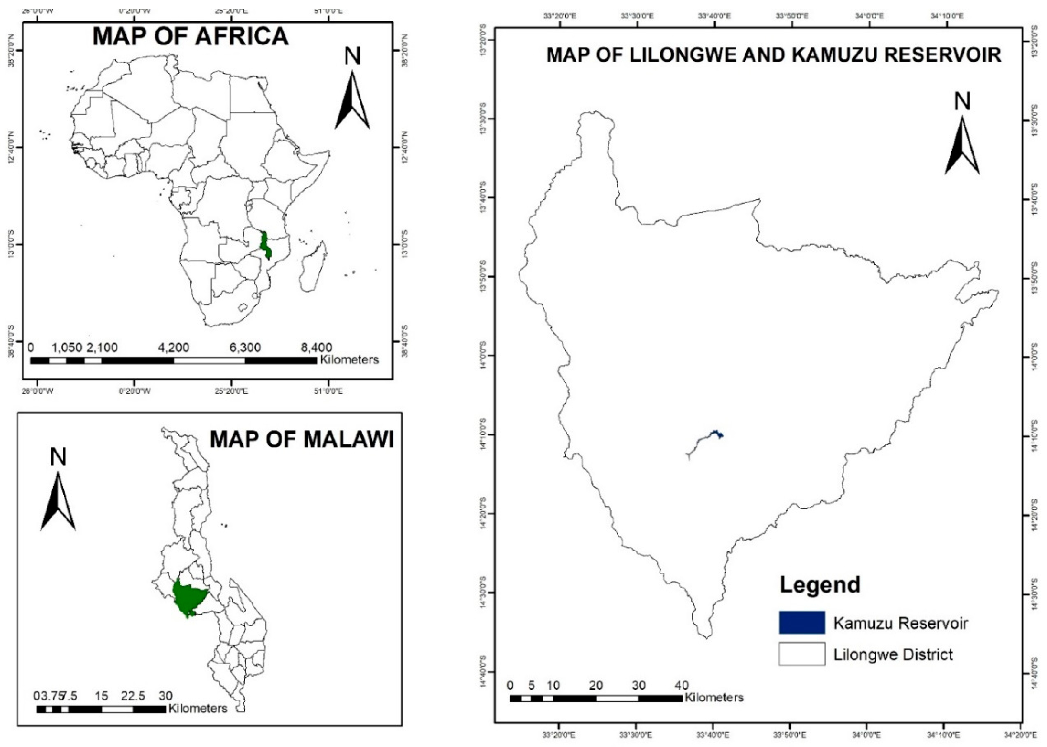
et al., 2016), and a lot of discharge from industrial, domestic, and agricultural activities end up in this river. The study was conducted on the Lilongwe River in the Lilongwe district of the central region of Malawi to understand the change in the water quality of the dam due to anthropogenic activities. Lilongwe district lies between 14.5
0 and 13.5
0 S latitude and between 33.5
0 and 34.5
0 E longitude (
Figure 1). Dzalanyama mountain range borders the country of Mozambique where the river originates. The river spans to a length of approximately 100 km with a catchment area of about 1800 km
2 (Nyasulu, 2012). There are two dams on the Lilongwe River which are used by the Lilongwe Water Board (LWB) for supplying water to the city. These are Kamuzu Dam I (14.17
0 S and 33.64
0 E) which was constructed on the Zambezi basin in 1966, have a capacity of 4,500,000 m
3, and Kamuzu Dam II (14.16
0 S and 33.68
0 E) which was constructed in 1989, just below Kamuzu Dam I, and later rehabilitated in 1992, has a capacity of 19,800,000m
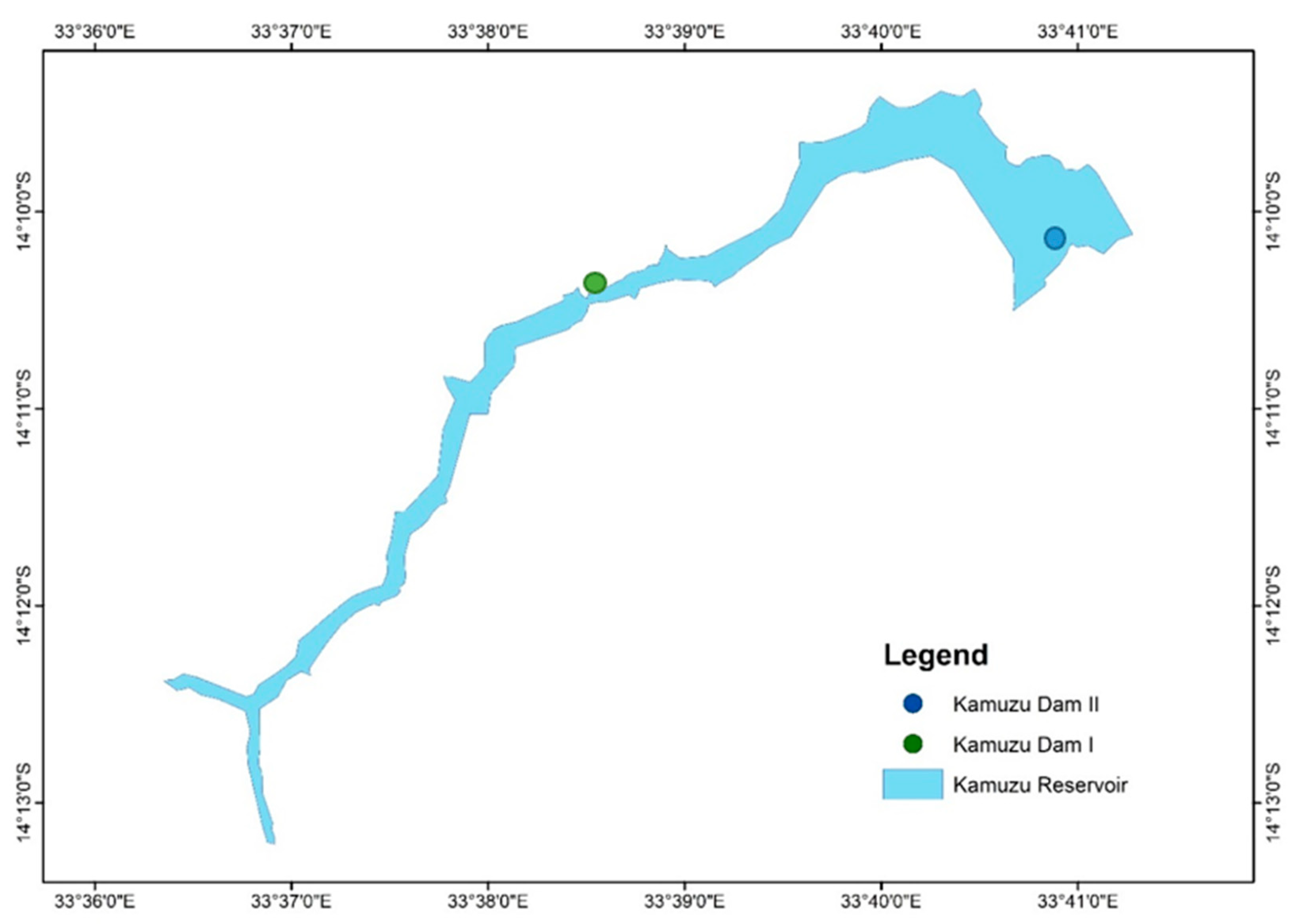
3. Kamuzu Dam I (KD-I) acts as a balancing reservoir and its outflow goes directly into Kamuzu Dam II (KD-II). The reservoir, named Kamuzu Reservoir (
Figure 2) was studied for the present work.
Some authors have studied the water quality of the area (Nyasulu, 2012) and its relationship with the landuse and landcover (Nkwanda et al., 2021), no study has been conducted to assess the variations in water quality parameters of the reservoir and estimation of water quality parameters using satellite images. In this study, the spatial spread of water quality parameters across the reservoir have been derived using the band ratio algorithm using satellite images and the same has been compared with the in-situ data.
3. Materials and Methods
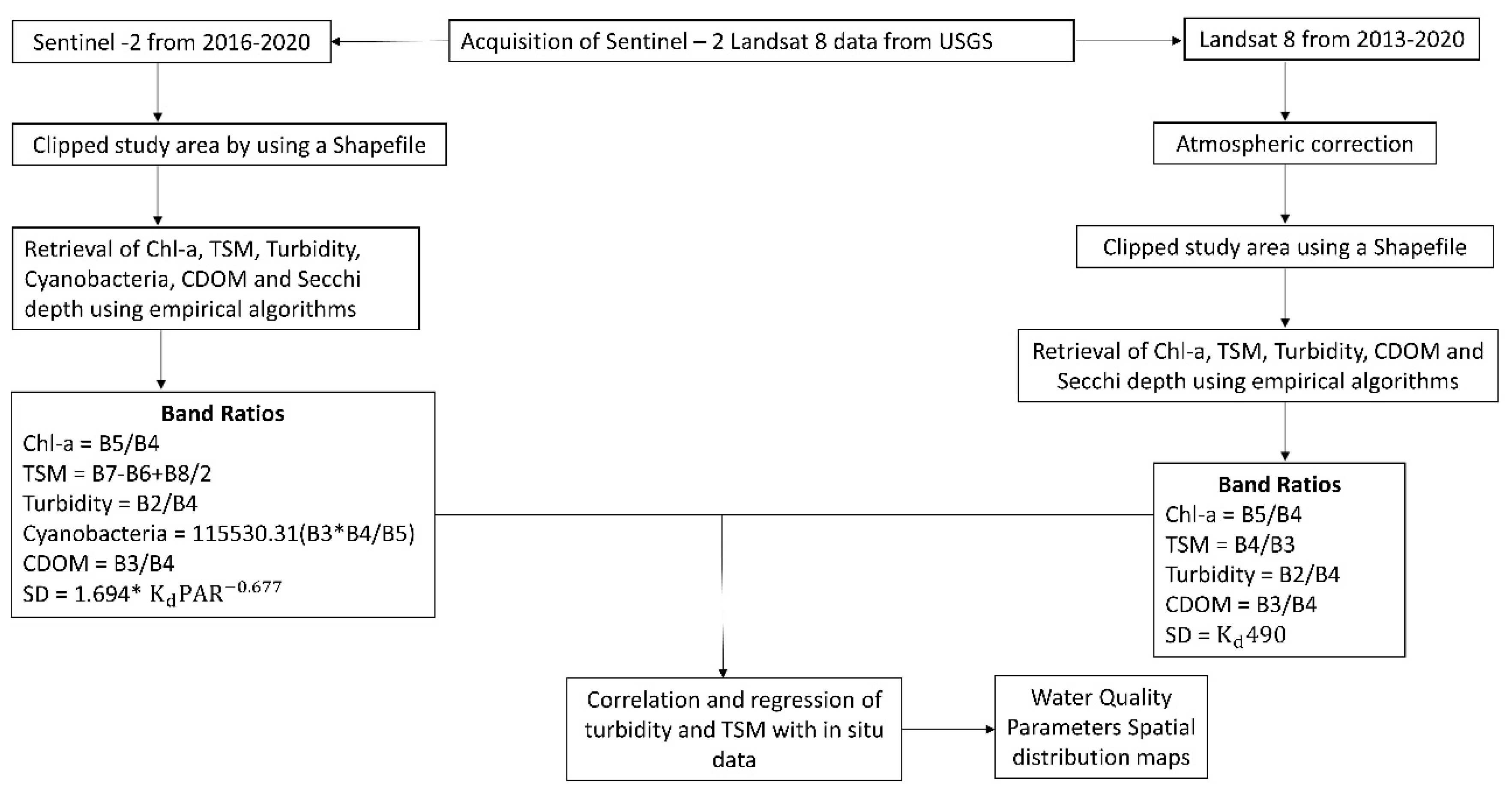
In the present study, the satellite data was used to estimate the water quality parameters which was compared with the in-situ data of the same period. The estimated and in-situ values were further analysed through corelation and regression. The flow chart followed in the study is shown in
Figure 3 which shows the different steps followed for the estimation of water quality using different band ratio for Landsat and Sentinel-2 data and its corelation with the in-situ data and the distribution of the water quality parameter in the reservoir. The satellite data (Sentinel-2 and Landsat 8 images) were downloaded from their respective websites (Copernicus
https://scihub.copernicus.eu/ for Sentinel-2 and Earth Explorer
https://earthexplorer.usgs.gov/ for Landsat 8). Atmospheric correction was applied to the Landsat 8 data, whereas for the Sentinel-2 data no such correction was applied, as it was already corrected for the effects of atmosphere. Both the data sets were clipped using a study-area shapefile to get the image for the study are only. Suitable band ratio algorithms (
Table 1) were applied to the images to estimate the water quality parameter.
The estimated results of water quality parameters from the algorithms were used in a correlation and regression analysis with in-situ data for obtaining the coefficient of determination (R2). For the values obtained from the processed images to correlate with in situ data, an average pixel value was extracted from a 5x5 pixel window corresponding to geographical coordinate of the water sampling point. This was necessary to avoid any bias in the estimated values, as a single pixel value may not represent the parameter value correctly.
3.1. Sentinel-2 MSI Data
Sentinel-2, which was launched in 2015, is a European wide-swath, high-resolution, multi-spectral imaging mission. It comprises of 2 twin satellites, sentinel-2A & 2B having a 5-day revisit frequency time. Sentinel-2 carries an optical instrument payload that samples 12 spectral bands: four bands at 10 m (Bands 2, 3, 4 and 8), six bands at 20 m (Bands 5, 6, 7, 8A, 11 and 12) and three bands at 60 m spatial resolution (Bands 1, 9 and 10). Cloud free Sentinel 2 Level 1C (L1C) MSI data for the study area for the study period has been downloaded which comprises of 100 sq. km tiles. A total 5 cloud free images (2016-2020) corresponding to the dates of the field sampling (±5 days) were downloaded and processed.
3.2. Landsat-8 Data
Landsat-8 is an American Earth Observation Satellite which was launched in 2013 which carries two sensors: the Operational Land Imager (OLI) and the Thermal Infrared Sensor (TIRS). OLI collects data in eight spectral bands (Bands 1-7 and 9) with a spatial resolution of 30 m. Band 8 collects the data with a spatial resolution of 15 m in a panchromatic band. TIRS measures thermal data at 100 m spatial resolution using two bands 10 and 11. Cloud free Landsat-8 images were downloaded from United States Geological Survey (USGS). These images were downloaded to match with the dates of Lilongwe Water Board field sampling data (±5 days). A total number of 7 cloud free (2013-2020) images corresponded to the field sampling dates were downloaded and processed.
3.3. Estimation of Water Quality Parameters Using Satellite Data
Kutser
et al., 2016 used the vegetation red edge and NIR in Sentinel-2 to estimate Total Suspended Matter (TSM) and obtained positive results. Gholizadeh,
et al., 2016, studied many possibilities of band math in Landsat 8 to estimate Chl-a, Secchi depth, Coloured Dissolved Organic Matter (CDOM), Total Suspended Matter (TSM), and Turbidity. Potes
et al., 2018, used the green and coastal aerosol bands and the green, blue and red bands in Sentinel-2 to map turbidity and cyanobacteria respectively in a reservoir. They concluded that Sentinel-2 had a high potential to monitor turbidity and cyanobacteria. Bresciani
et al., 2019, used Sentinel-2 and Landsat 8 to estimate chlorophyll-a, turbidity, and Secchi depth in two reservoirs. They used the Modular Inversion and Processing System to retrieve these parameters. Bande et al., 2018, compared Sentinel-2 and Landsat 8 to generate the effectiveness of one satellite over the other. They estimated that the concentration of chlorophyll-a using the coastal aerosol, blue, green and red bands while the blue and red bands were used to estimate turbidity. The results showed that Sentinel-2 had an edge over Landsat 8 data because of its better resolution. Soomets
et al., 2020, estimated TSM, Chl-a, Secchi depth, and CDOM from Sentinel-2 data using several band ratio algorithms. They obtained good results after comparison with in-situ data. The various band ratios used for the calculation of the water quality parameters, in the present study are listed in
Table 1. These ratios are based upon the above studies.
For Sentinel-2, R denotes the reflectance and the particular number after R denotes the wavelength. For Landsat 8, Rrs denotes the reflectance and Blue, Green, Red denotes the bands. Kd is the light attenuation coefficient.
Since the in-situ data was collected between the period of 2013 to 2020, Sentinel-2 satellite data could not be used for the entire study as it is only available from 2016. To corelate the data between 2013-2016, Landsat 8 data was used.
Cloud-free Landsat-8 satellite data of the Kamuzu reservoir were obtained for the period 2013 to 2020 and Sentinel-2 for the period 2016 to 2020. This period matched with the in-situ data collection dates. Landsat 8 images were pre-processed and processed in ERDAS Imagine and SNAP. Band ratio algorithms, as discussed above, were used to estimate the water quality parameters.
The resulting estimated parameters from the satellite images were correlated with in-situ water quality data to validate the results obtained from the satellite images while the other water quality parameters were illustrated as spatial distribution maps.
3.4. In-Situ Data
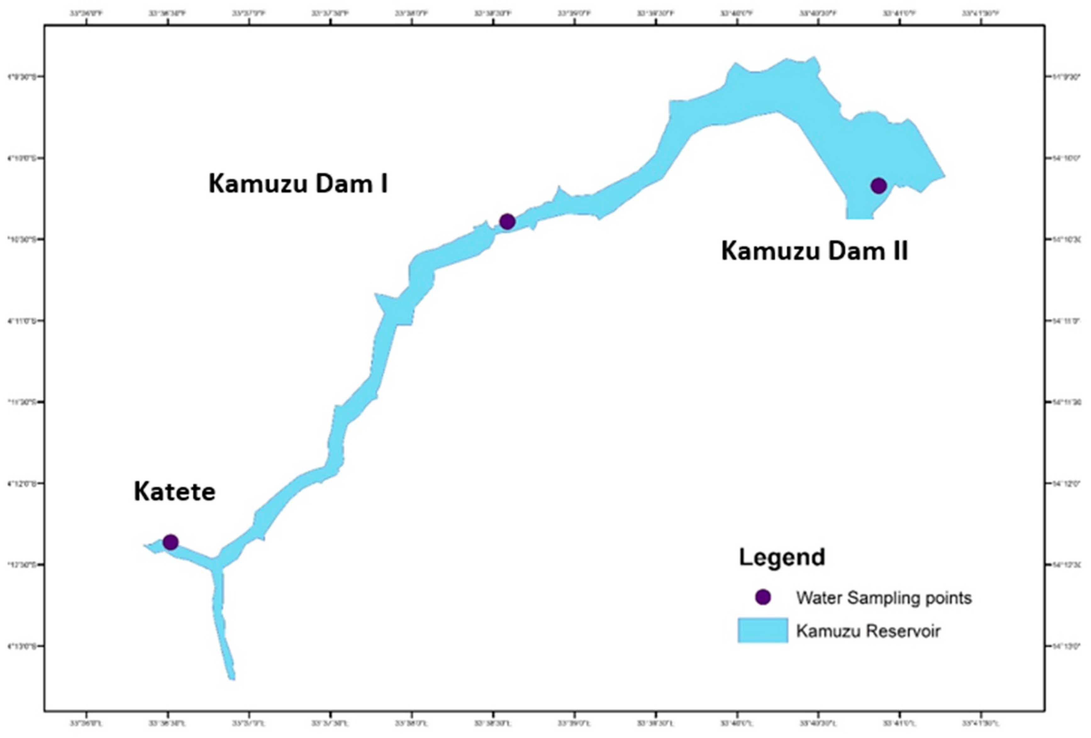
Lilongwe Water Board (LWB) is a Statutory Corporation established in 1947 as utility service provider and is responsible for the provision of water supply services to the City of Lilongwe and surrounding after abstracting raw water from the river through the two dams. The board periodically tests the water for various parameters at the source of the water and treated water. Field sampling data of the LWB was acquired which consisted of TSM and turbidity measured and the location of the sites from where the samples were collected. The LWB collects the data at 14 different points along the river. Out of the 14 data collection points, only 3 sampling points fall in the study area viz., Katete, Kamuzu Dam I (KD-I), and Kamuzu Dam II (KD-II) as shown in
Figure 4. The data ranged from 2013 to 2020, although the frequency of collection was inconsistent. The data obtained from LWB is shown in
Table 2.
Table 2.
In-situ data collected from LWB with name of the stations and the date.
Table 2.
In-situ data collected from LWB with name of the stations and the date.
The satellite images of the same dates for which the sample was collected was used for processing. However, for days when the cloud-free satellite image for the said date was not available, few days prior or post the date was selected and the cloud free image was downloaded and processed for estimation of water quality parameters. Care was taken so that no date of the satellite image is beyond 4 days of the sample collection date (
Table 3).
Field sampling dates corresponding with satellite imagery dates were also used to perform a correlation and regression analysis. Since only two parameters viz., TSM and turbidity were available for comparison, the correlation and regression analysis of the satellite image estimated TSM and turbidity, with the field-collected samples of TSM and turbidity were used to determine the coefficient of determination (R2).
4. Results and Discussion
The result of the estimated water quality parameter for the study is being presented in two parts. The first part describes the spatial distribution of the water quality parameters, as obtained from the satellite images using band-ratio algorithm. In the second part, the co-relation of the estimated parameters with the in-situ data has been done and the co-relation coefficient has been estimated to see the efficacy of the estimated water quality parameters vis-à-vis in-situ data.
4.1. Spatial Distribution of Estimated Parameters Using Sentinel-2 Data
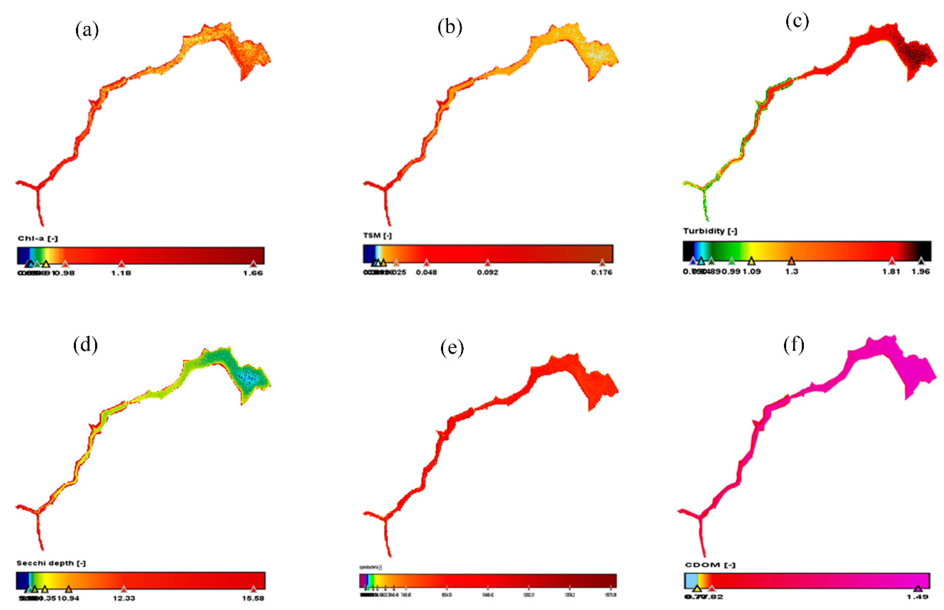
The Sentinel-2 satellite data was used to estimate six water quality parameters for the years 2016, 2017 and 2018.
Figure 5,
Figure 6, and
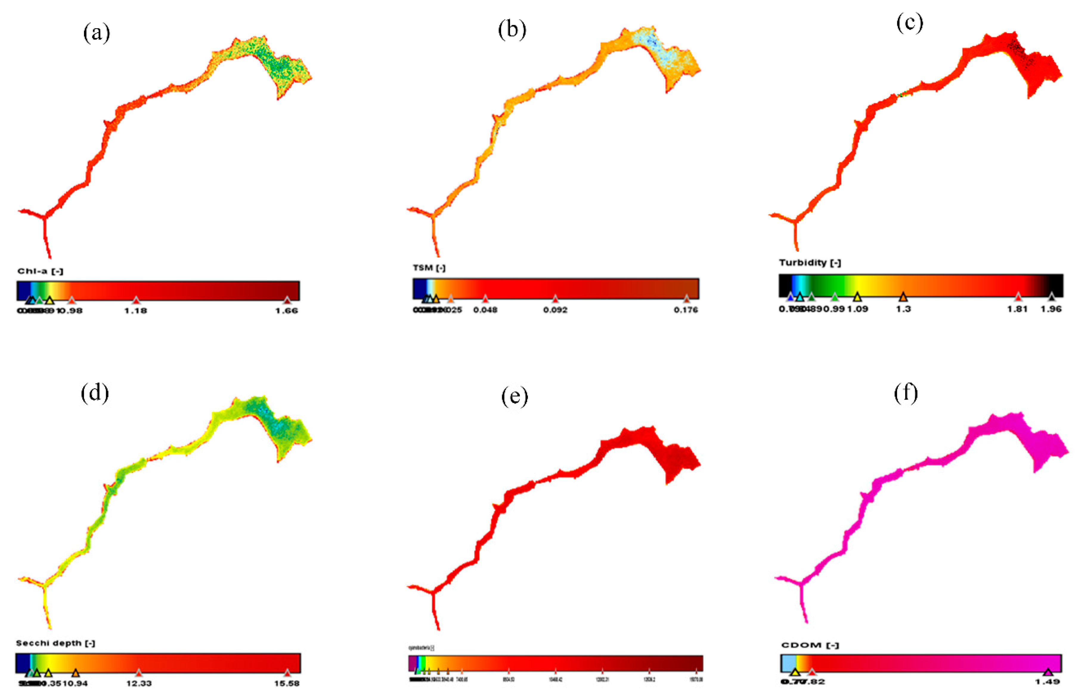
Figure 7 shows the spatial distribution of Chl-a, TSM, Turbidity, Secchi depth, Cyanobacteria and CDOM as estimated using Sentinel-2 images for the year 2016, 2017 and 2018 respectively.
Figure 5a shows that there is a high concentration of chlorophyll-a towards the Katete sampling point and some patches of high concentration towards KD-II. According to Gholizadeh, et al, 2016 there is a direct relationship between chlorophyll-a and cyanobacteria since cyanobacteria are capable of photosynthesis which needs chlorophyll for successful processing. The relationship is evident in figures 5a and 5e as both the parameters have higher concentration near Katete whereas it decreases for KD-I and KD-II sample points.
Figure 5b, 5c, and 5d, shows the spread of TSM, Secchi depth, and Turbidity. As can be seen that there are some patches of low concentration of TSM (
Figure 5b) towards the KD-I and II, and Secchi depth (
Figure 5d) is low for the same region whereas turbidity and Seechi depth shows a negative co-relation ((
Figure 5c and 5d). TSM and CDOM usually influence the scattering in the water which is evident from
Figure 5b and 5f. CDOM and TSM are in direct co-relation as both the values are high near southern tip of the water body whereas it is uniformly distributed in the northern region. Increase in turbidity relates to less of planktons and hence less of dissolved oxygen and Chl-a, which is also observed in
Figure 5a and 5c.
Figure 6a-f shows the spatial distribution of the estimated water quality parameters for 2017 using the Sentinel image of 16
th September 2017. The observation is similar to the observation of 2016. As per the
Figure 6a, there is a high concentration of chlorophyll-a around the Katete sampling region, but the concentration is low towards KD-II.
Figure 6b shows the distribution of total suspended matter and is high at the southern part whereas it reaches to a minimum in the northern part near KD-II. The spatial distribution of turbidity is represented in
Figure 6c which is almost similar and on the mid-high side for the entire study area, except for the northern region where it is maximum. This is also reflected in the Seechi depth spatial distribution in
Figure 6d. For most of the region the values are moderate whereas for the northern region the values are very less (wherever there is a higher value of turbidity). Cyanobacteria and CDOM distribution are almost uniform throughout the reservoir. Except for
Figure 6e and f, all other distribution follows the conventional patterns i.e., wherever there is more turbidity, the seechi depth is less representing not so clear water, less of Chl-a because of less dissolved oxygen and less of planktons.
The results obtained in
Figure 7 for the year 2018 are similar to those in
Figure 5 and
Figure 6 for years 2016 and 2017 respectively. The relationships observed between water parameters are similar to the earlier years.
The three Sentinel-2 processed figures (
Figure 5,
Figure 6, and
Figure 7) have shown variation in the Chl-a values. The estimated spatial distribution of Chl-a for 2017 and 2018 are almost similar. However, when Chl-a values are compared with 2016, it shows a major change in chlorophyll-a concentration for KD-II sampling point but almost similar values for Katete and KD-I, which has lower concentrations. The high concentrations of Chl-a are observed from Katete running towards KD-I and is similar for all the three years for which the study has been done. The high concentration around Katete and KD-I region can be attribute to the fact that there are settlements and agricultural activities around the region and agricultural and domestic wastes ends up in the water leading to high concentrations of Chl-a. The values of Chl-a decreases northwards as there are less settlements around the dam area and almost no effluents are passed onto the water body. However, the concentration of Chl-a in 2016 in the northern region was almost similar to that of southern part, which needs to be studied in more detail.
The figures also show the relationship that is there between Secchi depth, turbidity, and TSM. All the figures show a direct relationship between Secchi depth and TSM while there is an inverse relationship between Secchi depth and turbidity. The depth of water transparency is low towards the KD-II compared to the KD-I and Katete sampling regions, at the same time TSM concentration is low while turbidity concentration is high.
4.2. Spatial Distribution of Estimated Parameters Using Landsat Data
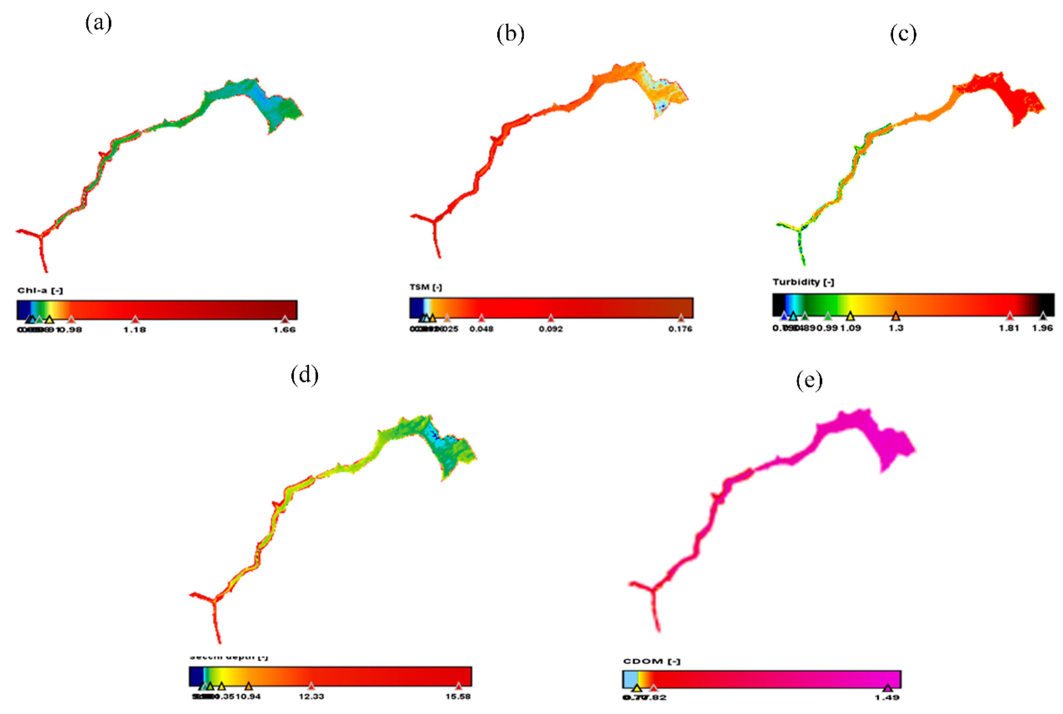
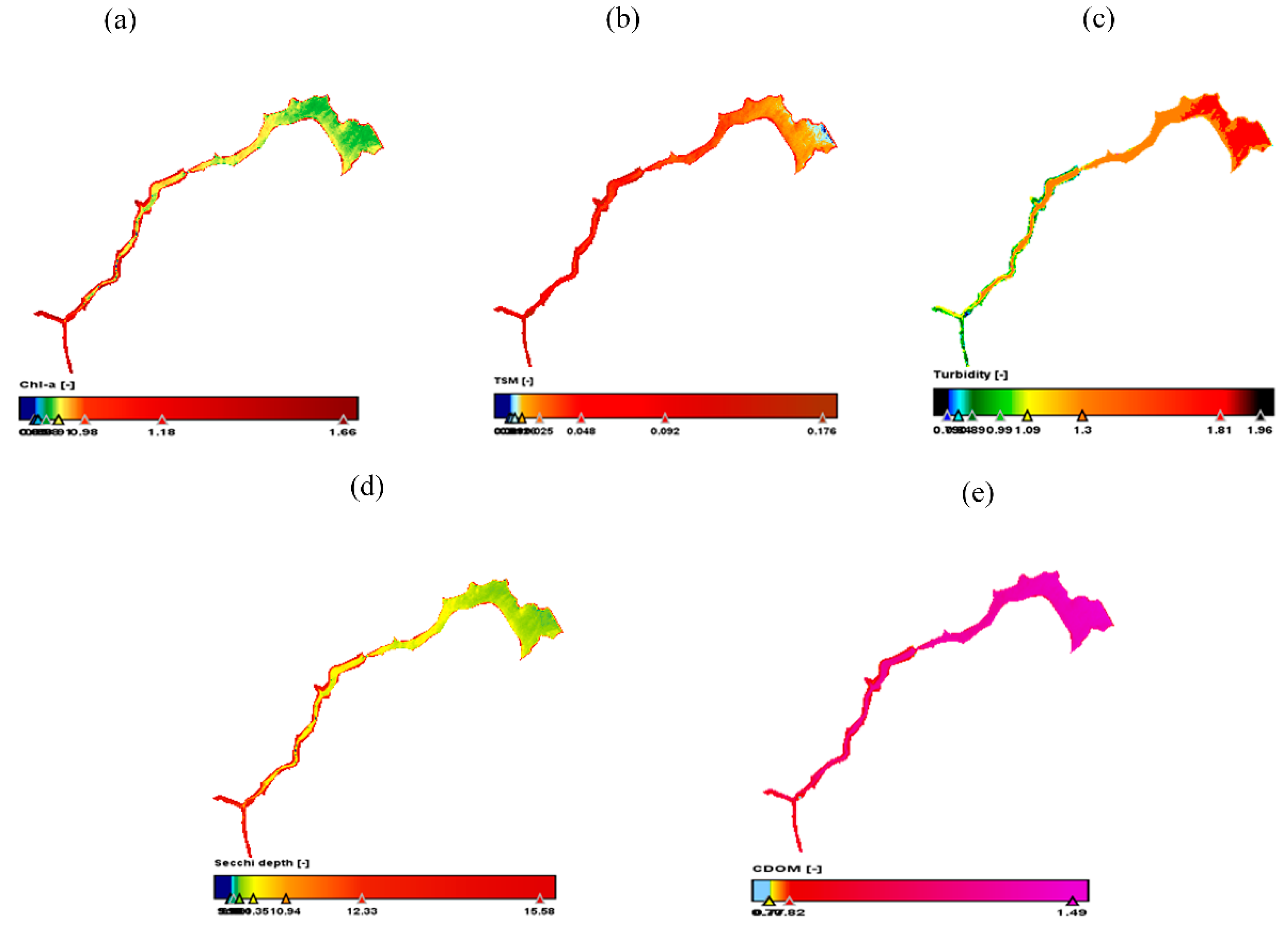
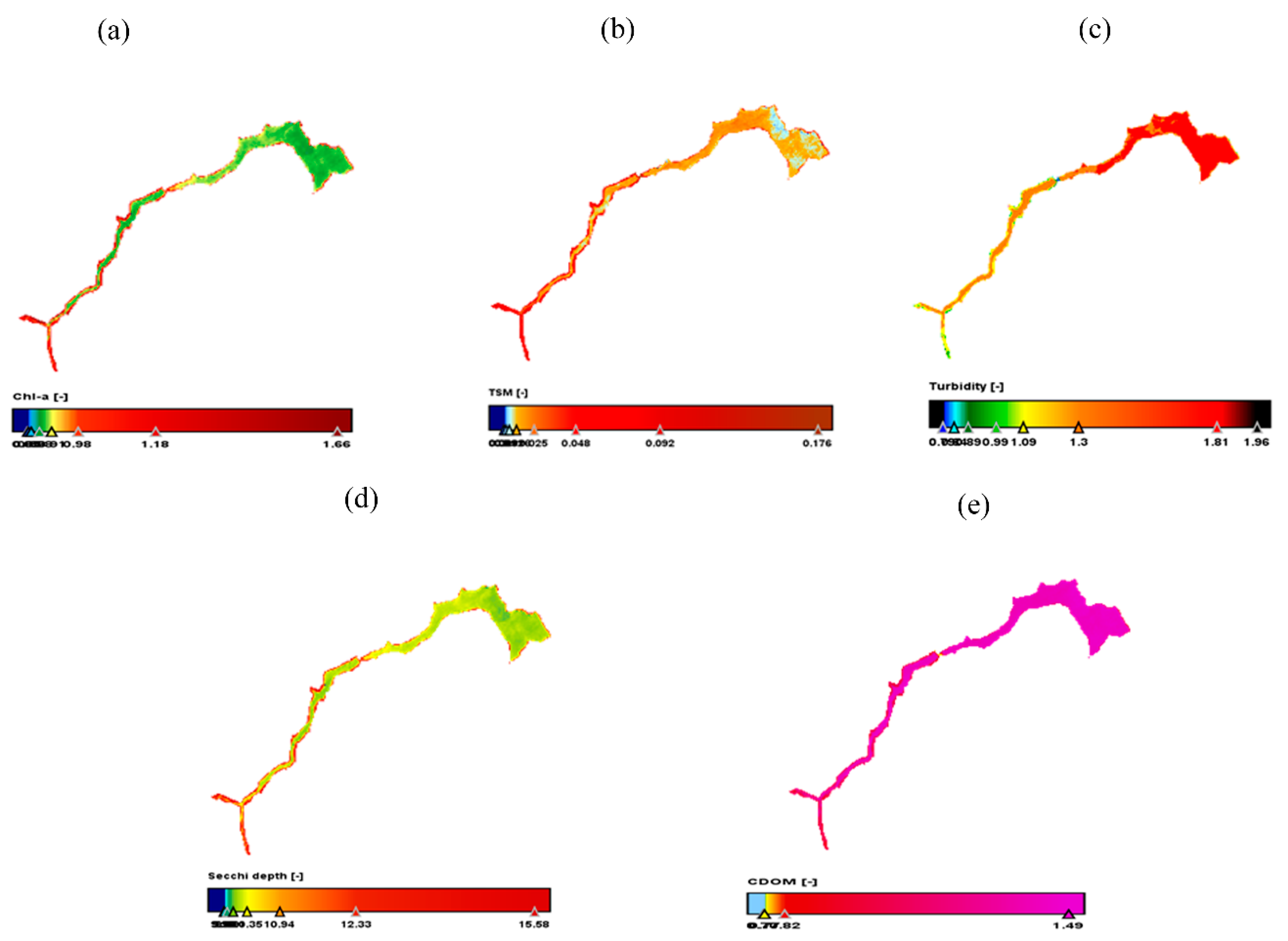
Landsat-8 satellite data was used to estimate five water quality parameters for the years 2013, 2014 and 2019. Figure. 8, 9, and 10 show the spatial distributions of Chl-a, TSM, Turbidity, Seechi depth and CDOM, as estimated from the Landsat-8 data. The spatial distribution of these parameters for all the years are almost similar as can be observed in the figures. The Chl-a distribution indicates a high concentration towards the Katete sampling region but has a low concentration towards the KD-I & II. CDOM distribution shows a low concentration near Katete which increases towards KD-I and increases further towards KD-II and remains almost uniform near KD-II. Turbidity and Seechi depth distribution shows an inverse relationship, which is expected, and turbidity increases from Katete to KD-I and further towards KD-II and corresponding Seechi depth decreases from Katete towards KD-I and further to KD-II. TSM and turbidity also follows an inverse relationship for the region between Katete and KD-I, however, for the area around KD-II, the turbidity has a very high value, but the TSM does not vary accordingly. There are some patches in the area around KD-II where the TSM varies from moderate to low which is also reflected similarly in the distribution of Seechi depth. Few patches of low concentration of TSM and Seechi depth near the KD-II sampling point needs to be investigated more, as all other parameters are distributed as expected.
Comparing the results of parameters between the time series, the Chl-a is almost similar for Katete between 2013, 2014 and 2019. However, the value increases for 2014 from 2013 and then it decreases for 2019. CDOM values for all the years are similar for all the observation stations and are more or less uniform over the period. Turbidity is least at Katete station for all the years but has increase over time. For KD-I, the turbidity increases as compared to Katete and further increases around the observation point KD-II. Turbidity in the northern region near KD-II is maximum for all the years but decreases in 2014 as compared to 2013 but again increases in 2019. For all the years, Seechi depth is inversely related with the turbidity and same is the case with TSM.
4.3. Validation of the Estimated Data vs In-Situ Data Using Co-Relation and Regression Analysis
As stated earlier, only two data viz., turbidity and TSM were common between the estimated and in-situ data collected for the study area between the study period. A co-relation and regression analysis was performed between the two data to understand the efficacy of the satellite image derived water quality parameters and whether these could replace the manual and tedious data collection procedure. In-situ data were available for 3 sampling points over a period resulting in 15-20 data points to be validated depending upon the availability of the cloud free satellite data. For all the sample points the TSM and Turbidity values were read from the satellite generated TSM and Turbidity spatial distribution maps (
Figure 5,
Figure 6,
Figure 7,
Figure 8,
Figure 9 and
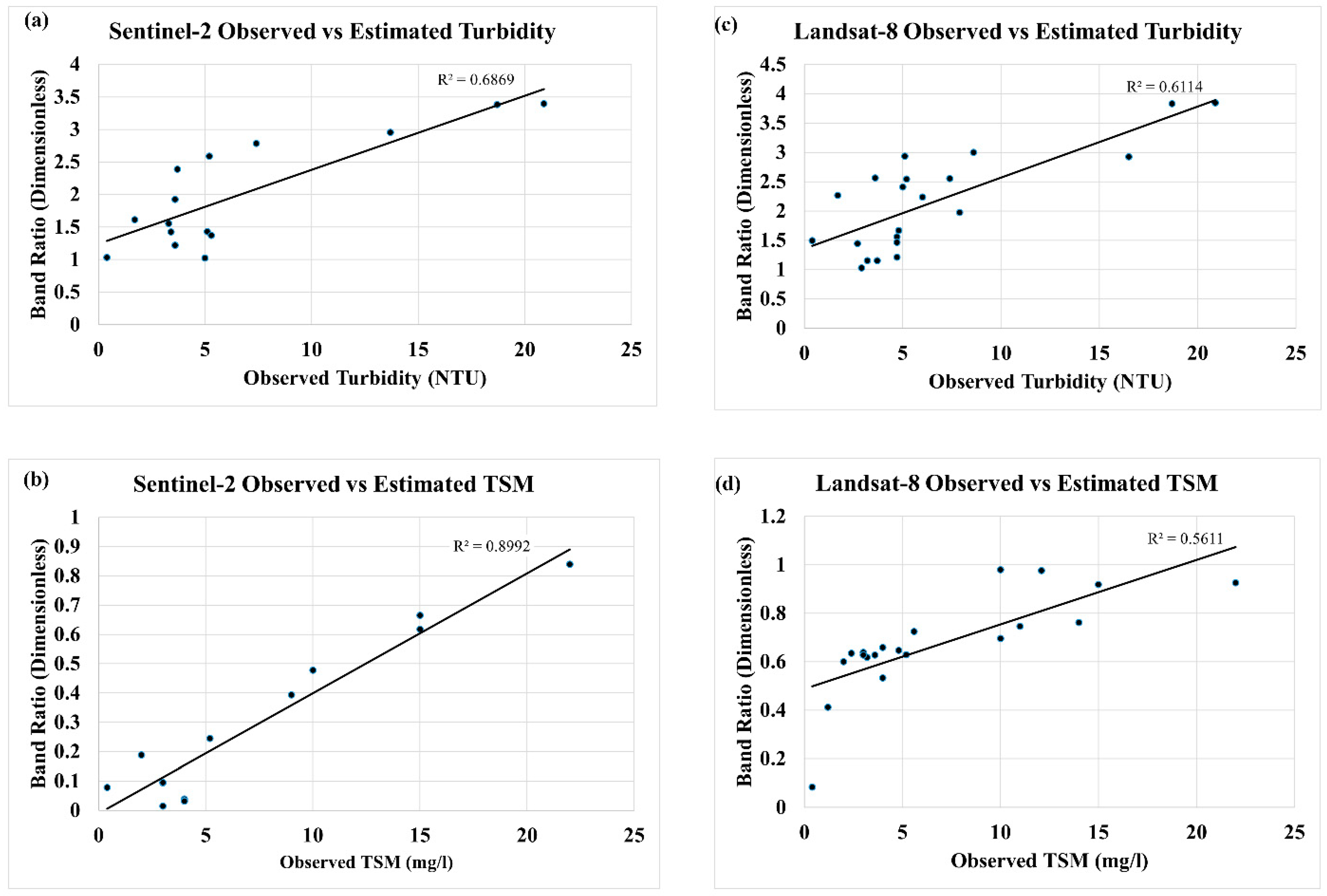
Figure 10). Since these estimated data were found using band-ratio algorithms, the resultant values were dimensionless. A co-relation graph between the observed and estimated values were plotted, as shown in
Figure 11.
Figure 11 (a) and (b) are the co-relation curve for Sentinel-2 data vis-à-vis observed values as obtained by field sampling whereas
Figure 11 (c) and (d) is that of Landsat-8. It was observed that the co-relation co-efficient of TSM is 0.9 (
Figure 11(b)) and that of turbidity is 0.7 (
Figure 11 (a)). The same for Landsat-8 was found to be 0.6 (
Figure 11 (c)) and 0.56 (
Figure 11 (d)) respectively. As the turbidity and TSM values shows a strong co-relation for Sentinel-2 data as compared to the Landsat-8 data, the same may be used to estimate the TSM and turbidity values to a reasonable accuracy. However, the number of sample points were less, nonetheless, it can be concluded that Sentinel-2 satellite data and band-ratio algorithms can be used to fairly estimate the water quality parameters for a large water body as has also been reported by several other studies. The better accuracy of Sentinel-2 is a result of the better spatial resolution of the satellite data than the Landsat-8 data. Since the observed samples over the years were not tested for other parameters and hence the estimated values could not be compared, but a fair assessment of the parameters can be done using satellite data.
The variation in the estimated data for some of the parameters at few locations may be attributed to the fact that the water body under study is a fairly large water body and the samples were taken only from the banks of the river and the dam, whereas the satellite data used in the study was of 10m and 30m spatial resolution spread over the entire dam. Better spatial resolution such as 5m or 1m satellite data may result in better estimation of the water quality parameters.
5. Conclusions
Remote sensing is an effective way through which some of the challenges faced in water quality monitoring can be solved. From the results obtained through co-relation analysis of TSM and turbidity retrieved from Sentinel 2 and the in-situ data, it has been observed that a reliable precision can be obtained using estimation of turbidity and TSM from satellite images. Although Landsat 8 was also used to estimate TSM and turbidity, the co-relation results shows that the parameters estimated using Sentinel 2 were significantly better than Landsat 8, because of better spatial resolution. It can be concluded that remotely sensed data can result in effective water quality monitoring.
The results also shows that Sentinel 2 and Landsat 8 data has great potential for estimating water quality parameters as it was possible to estimate and map Chl-a, TSM, turbidity, cyanobacteria, and CDOM concentrations as well the Secchi depth using band ratio algorithms. The water quality can be estimated and assessed on a wider range through spatial distribution maps. This study further shows that remote sensing can address the problem of limited in situ data. The frequency of in situ samplings is also a problem that was witnessed in the number of times data was collected over 7 years. With Sentinel 2 and Landsat 8 having short revisit times of 5 and 16 days respectively, they come as a solution to this problem.
The results in this study have also shown that the highest concentrations of all the water parameters in the reservoir is at the upstream region where Katete is situated to where the Kamuzu Dam I is, as compared to the region between Kamuzu dam I and Kamuzu dam II. This is the region where the population is high compared to all the other regions of the catchment of the two reservoirs. Many anthropogenic activities occur around this area, the most common one being farming. The reservoir hence acts as drainage for most of the agricultural effluents when they are washed off by runoff.
The authors used offline processing of downloaded satellite images which took considerable amount of time. However, with historical and current satellite data at varying resolutions and processing tools available on Google Earth Engine (GEE) platform, water quality assessments have become much simpler and faster. A detailed study of the region about seasonal variation of water quality parameters with anthropogenic activities may be undertaken using GEE to understand the effect of these activities on the changing water quality of the reservoir.
Acknowledgments
The authors would like to thank the Water Quality Officer, Mr. Charles Kachingwe, of Lilongwe Water Board (LWB), Malawi for assistance in acquiring the in-situ data and the permission to use the data in this paper. BC would also like to thank the Government of Malawi for sponsoring him for the post-graduate program in Sharda University, during which the work was carried out. SP is thankful to Ms Sakshi Rai for helping in preparing the final diagrams.
References
- Ansper, A. and Alikas, K. (2018) ‘Retrieval of Chlorophyll a from Sentinel-2 MSI Data for the European Union Water Framework Directive Reporting Purposes’, Remote Sensing, 11(1), p. 64. [CrossRef]
- Bande, Prosper, Elhadi Adam, Mohamed A. M. Abd Elbasit, Samuel Adelabu (2018). Comparing landsat 8 and sentinel-2 in mapping water Quality at Vaal Dam. Paper published in IGRASS 2018 conference by IEEE.
- Bresciani, Mariano, Claudia Giardino, Daniela Stroppiana, Maria Antonietta Dessena, Paola Buscarinu, Loretta Cabras, Karin Schenk, Thomas Heege, Hendrik Bernet, Giorgos Bazdanis & Apostolos Tzimas (2019) Monitoring water quality in two dammed reservoirs from multispectral satellite data, European Journal of Remote Sensing, 52:sup4, 113-122. [CrossRef]
- Cherif, E. K., Salmoun, F. and Mesas-Carrascosa, F. J. (2019) ‘Determination of Bathing Water Quality Using Thermal Images Landsat 8 on the West Coast of Tangier: Preliminary Results’, Remote Sensing, 11(8), p. 972. [CrossRef]
- Chen, Junde, Defu Zhang, Shuangyuan Yang, Yaser Ahangari Nanehkaran (2020). Intelligent monitoring method of water quality based on image processing and RVFL-GMDH model. IET Image Process., 2020, Vol. 14 (17), pp. 4646-4656. [CrossRef]
- Chidya, R. C., Mulwafu, W. O., & Banda, S. C. (2016). Water supply dynamics and quality of alternative water sources in low-income areas of Lilongwe City, Malawi. Physics and Chemistry of the Earth, Parts A/B/C, 93, 63–75. [CrossRef]
- Chimwanza, B., Mumba, P.P., Moyo, B.H.Z. and Kadewa, W. (2006). The impact of farming on river banks on water quality of the rivers. Int. J. Environ. Sci. Technol. [CrossRef]
- Elhag, Mohamed, Ioannis Gitas, Anas Othman, Jarbou Bahrawi and Petros Gikas (2019). ‘Assessment of Water Quality Parameters Using Temporal Remote Sensing Spectral Reflectance in Arid Environments, Saudi Arabia’, Water, 11, 556, pp 1-14. [CrossRef]
- Gholizadeh, M., Melesse, A. and Reddi, L. (2016) ‘A Comprehensive Review on Water Quality Parameters Estimation Using Remote Sensing Techniques’, Sensors, 16(8), p. 1298. [CrossRef]
- Goldar, B. and Banerjee, N. (2004) ‘Impact of informal regulation of pollution on water quality in rivers in India’, Journal of Environmental Management, 73(2), pp. 117–130. [CrossRef]
- Katlane, R., Cecile Dupouy, Jean Claude Berges and Anna Mannai (2020) Estimation of Chl-a conc in estarine water of Kneiss Archpileago gulf of Gabes using Sentinel-2A and EO1 data. Paper published in IEEE conference M2GRASS 2020.
- Khan, Mashhood Ahmad and Ghouri, Arsalan Mujahid, (2011). Environmental Pollution: Its Effects on Life and Its Remedies. Researcher World: Journal of Arts, Science & Commerce, Vol. 2, No. 2, pp. 276-285, 2011, Available at SSRN: https://ssrn.com/abstract=1981242.
- Kim, Yong Hoon, Seunghyun Son, Hae-Cheol Kim, Bora Kim, Young-Gyu Park, Jungho Nam and Jongseong Ryud (2020). ‘Application of satellite remote sensing in monitoring dissolved oxygen variabilities: A case study for coastal waters in Korea Application of Sentinel 2 MSI Images to Retrieve Suspended Particulate Matter Concentrations in Poyang Lake’, Environment International, 134, 105301, pp 1-10. [CrossRef]
- Kutser, Tiit, Gema Casal Pascual, Claudio Barbosa, Birgot Paavel, RenatoFerreira, Lino Carvalho & Kaire Toming (2016) Mapping inland water carbon content with Landsat 8 data, International Journal of Remote Sensing, 37:13, 2950-2961. [CrossRef]
- Nkwanda, I.S., Feyisa, G.L., Zewge, F., and Makwinja, R. (2021). Impact of land-use/land-cover dynamics on water quality in the Upper Lilongwe River basin, Malawi. Int J Energ Water Res 5, 193–204. [CrossRef]
- Nyasulu, T.H. (2012) ‘Assessment of the Quality of Water in Urban Rivers-A case study of Lilongwe River in Malawi, Unpublished MS thesis available at https://catalog.ihsn.org/index.php/citations/33290 (last accessed June 2022).
- Peppa, M., Vasilakos, C. and Kavroudakis, D. (2020) ‘Eutrophication Monitoring for Lake Pamvotis, Greece, Using Sentinel-2 Data’, ISPRS International Journal of Geo-Information, 9(3), p. 143. [CrossRef]
- Pereira, L. S. F., Andes, L.C., Cox, A.L. and Ghulam, A (2018). ‘Measuring Suspended-Sediment Concentration and Turbidity in the Middle Mississippi and Lower Missouri Rivers Using Landsat Data’, JAWRA Journal of the American Water Resources Association, 54(2), pp. 440–450. [CrossRef]
- Phiri, O., Mumba, P., Moyo, B.H.Z. and Kadewa, W. (2005) ‘Assessment of the impact of industrial effluents on water quality of receiving rivers in urban areas of Malawi’, International Journal of Environmental Science & Technology, 2(3), pp. 237–244. [CrossRef]
- Potes, M., Rodrigues, G., Penha, A.M., Novais, M.H., Costa, M.J., Salgado, Rui and Morais, M.M. (2018). ‘Use of Sentinel 2 – MSI for water quality monitoring at Alqueva reservoir, Portugal’, Proceedings of the International Association of Hydrological Sciences, 380, pp. 73–79. [CrossRef]
- Sagan, V., Kyle T. Peterson, Maitiniyazi Maimaitijiang, Paheding Sidike, John Sloan, Benjamin A. Greeling, Samar Maalouf, Craig Adams (2020). Monitoring inland water quality using remote sensing: potential and limitations of spectral indices, bio-optical simulations, machine learning, and cloud computing, Earth-Science Reviews, Volume 205, 103187. [CrossRef]
- Shi, Kun, Yunlin Zhang, Yibo Zhang, Boqiang Qin, Guangwei Zhu (2020). Understanding the long-term trend of particulate phosphorus in a cyanobacteria-dominated lake using MODIS-Aqua observations. Science of the Total Environment 737 (2020) 139736. [CrossRef]
- Sicard, C., Glen, C., Aubie, B., Wallace, D., Jahanshahi-Anbuhi, S., Pennings, K., Daigger, G.T., Pelton, R., Brennan, J.D. and Filipe, C.D.M. (2015). ‘Tools for water quality monitoring and mapping using paper-based sensors and cell phones’, Water Research, 70, pp. 360–369. v.
- Silva, M. G. G.; D. J. Silva; P. D. Costa; R. C. Silva; T. E. B. Cassimiro; L. S. Amorim; D. A. Rocha; Z. M. A. Peixoto (2021). Analysis of water quality at hydrographic basin scale using satellite images, co-occurrence matrices and Bayes classifier. Water Supply 21 (8): 4418–4428. [CrossRef]
- Soomets, T., Uudeberg, K, Jakovels, D., Brauns, A., Zagars, M. and Kutser, T. (2020). ‘Validation and Comparison of Water Quality Products in Baltic Lakes Using Sentinel-2 MSI and Sentinel-3 OLCI Data’, Sensors, 20(3), p. 742. [CrossRef]
- Stevenson, A. H. (1953) ‘Studies of Bathing Water Quality and Health’, American Journal of Public Health and the Nations Health, 43(5_Pt_1), pp. 529–538. [CrossRef]
- Toming, Kaire, Tiit Kutser, Alo Laas, Margot Sepp, Birgot Paavel, and Tiina Nõges. 2016. "First Experiences in Mapping Lake Water Quality Parameters with Sentinel-2 MSI Imagery" Remote Sensing 8, no. 8: 640. [CrossRef]
- Topp, S.N., Tamlin M. Pavelsky, Daniel Jensen, Marc Simard and Matthew R. V. Ross (2020). Research Trends in the Use of Remote Sensing for Inland Water Quality Science: Moving Towards Multidisciplinary Applications. Water 2020, 12 169. [CrossRef]
- Zheng, Z., Ren, J., Li, Y., Huang, C., Liu, Ge, Du, C. and Lyu, H. (2016). ‘Remote sensing of diffuse attenuation coefficient patterns from Landsat 8 OLI imagery of turbid inland waters: A case study of Dongting Lake’, Science of The Total Environment, 573, pp. 39–54. [CrossRef]
Figure 1.
Locator Map of Study Area.
Figure 1.
Locator Map of Study Area.
Figure 2.
Kamuzu Reservoir along Lilongwe River, Central Malawi, and the location of the Dams.
Figure 2.
Kamuzu Reservoir along Lilongwe River, Central Malawi, and the location of the Dams.
Figure 3.
Methodology flowchart showing different steps.
Figure 3.
Methodology flowchart showing different steps.
Figure 4.
Water Sample points on the study area.
Figure 4.
Water Sample points on the study area.
Figure 5.
Sentinel 2 spatial distribution maps showing (a) chlorophyll-a, (b) TSM, (c) Turbidity, (d) Secchi depth, (e) Cyanobacteria, and (f) CDOM for 2nd August 2016.
Figure 5.
Sentinel 2 spatial distribution maps showing (a) chlorophyll-a, (b) TSM, (c) Turbidity, (d) Secchi depth, (e) Cyanobacteria, and (f) CDOM for 2nd August 2016.
Figure 6.
Sentinel 2 spatial distribution maps showing (a) chlorophyll-a, (b) TSM, (c) Turbidity, (d) Secchi depth, (e) Cyanobacteria, and (f) CDOM for 16th September 2017.
Figure 6.
Sentinel 2 spatial distribution maps showing (a) chlorophyll-a, (b) TSM, (c) Turbidity, (d) Secchi depth, (e) Cyanobacteria, and (f) CDOM for 16th September 2017.
Figure 7.
Sentinel 2 spatial distribution maps showing (a) chlorophyll-a, (b) TSM, (c) Turbidity, (d) Secchi depth, (e) Cyanobacteria, and (f) CDOM for 3rd July 2018.
Figure 7.
Sentinel 2 spatial distribution maps showing (a) chlorophyll-a, (b) TSM, (c) Turbidity, (d) Secchi depth, (e) Cyanobacteria, and (f) CDOM for 3rd July 2018.
Figure 8.
Landsat 8 spatial distribution maps showing (a) Chlorophyll-a, (b) TSM, (c) Turbidity, (d) Secchi depth, and (e) CDOM for September 2013.
Figure 8.
Landsat 8 spatial distribution maps showing (a) Chlorophyll-a, (b) TSM, (c) Turbidity, (d) Secchi depth, and (e) CDOM for September 2013.
Figure 9.
Landsat 8 spatial distribution maps showing (a) Chlorophyll-a, (b) TSM, (c) Turbidity, (d) Secchi depth, and (e) CDOM for October 2014.
Figure 9.
Landsat 8 spatial distribution maps showing (a) Chlorophyll-a, (b) TSM, (c) Turbidity, (d) Secchi depth, and (e) CDOM for October 2014.
Figure 10.
Landsat 8 spatial distribution maps showing (a) Chlorophyll-a, (b) TSM, (c) Turbidity, (d) Secchi depth, and (e) CDOM for September 2019.
Figure 10.
Landsat 8 spatial distribution maps showing (a) Chlorophyll-a, (b) TSM, (c) Turbidity, (d) Secchi depth, and (e) CDOM for September 2019.
Figure 11.
Co-relation graph between observed and estimated values of TSM and turbidity for Landsat-8 and Sentinel-2 satellite data.
Figure 11.
Co-relation graph between observed and estimated values of TSM and turbidity for Landsat-8 and Sentinel-2 satellite data.
Table 1.
Band ratios used to retrieve Chl-a, TSM, Turbidity, CDOM, SD and Cyanobacteria from satellite images.
Table 1.
Band ratios used to retrieve Chl-a, TSM, Turbidity, CDOM, SD and Cyanobacteria from satellite images.
| Sentinel-2 |
Landsat 8 |
| Band ratio |
Water Quality Parameter |
Reference |
Band ratio |
Water Quality Parameter |
Reference |
| R704/R664 |
Chl-a |
(Ansper and Alikas, 2018) |
Rrs(NIR)/ Rrs(Red) |
Chl-a |
(Gholizadeh, et al., 2016) |
| R782-R740+R832/2 |
TSM |
(Soomets et al., 2020) |
Rrs(Red)/ Rrs(Green) |
TSM |
(Gholizadeh, et al., 2016) |
| R492/R664 |
Turbidity |
(Bande et al., 2018) |
Rrs(Blue)/ Rrs(Red) |
Turbidity |
(Bande et al., 2018) |
| R559/R664 |
CDOM |
(Toming et al., 2016) |
Rrs(Green)/
Rrs(Red) |
CDOM |
(Toming et al., 2016) |
| 1.694*KdPAR-0.677
|
SD |
(Soomets et al., 2020) |
Kd490 |
SD |
(Zheng et al., 2016) |
| 115530.31*(R559*R664)/R704 |
Cyanobacteria |
(Potes et al., 2018) |
|
|
|
Table 3.
Number of days difference between the sample date and image date.
Table 3.
Number of days difference between the sample date and image date.
Sample collection date
(mm/dd/yyyy)
|
Image difference in days
(+ is for advanced and – for prior date)
|
| 10/09/2013 |
2 |
| 04/10/2014 |
-3 |
| 15/06/2016 |
1 |
| 04/08/2016 |
-1 |
| 07/08/2018 |
2 |
| 09/09/2019 |
4 |
| 31/10/2019 |
0 |
|
Disclaimer/Publisher’s Note: The statements, opinions and data contained in all publications are solely those of the individual author(s) and contributor(s) and not of MDPI and/or the editor(s). MDPI and/or the editor(s) disclaim responsibility for any injury to people or property resulting from any ideas, methods, instructions or products referred to in the content. |
© 2023 by the authors. Licensee MDPI, Basel, Switzerland. This article is an open access article distributed under the terms and conditions of the Creative Commons Attribution (CC BY) license (http://creativecommons.org/licenses/by/4.0/).

