
Submitted:
26 January 2024
Posted:
29 January 2024
Read the latest preprint version here
Abstract
A statistical simulation is presented which reproduces the correlation obtained from EPR coincidence experiments without non-local connectivity. In addition to the spin polarization, we identify spin coherence as an attribute, and complementary to polarization, which is anti-symmetric and generates the helicity. This changes the point particle spin to a structured one with two orthogonal magnetic moments of spin $\frac{1}{2}$ each. They couple in free flight to form a spin 1, a boson. Upon encountering a filter, the boson decouples into its two independent spins axes of $\frac{1}{2}$, with one aligning with the filter and the other randomizing. The process of decoupling from a free-flight boson to a measured fermion is responsible for the quantum correlation which results in the observed violation of Bell's Inequalities. The only variable in this work is the angle that orients a spin on the Bloch sphere, first identified in the 1920's. The new features introduced here result from changing the spin symmetry from SU(2) to the quaternion group, $Q_8$.
Keywords:
foundations of physics
; dirac equation
; spin
; quantum theory
; non-locality
; helicity
Introduction
We consider the correlation obtained from coincidence EPR experiments [1,2,3]. An EPR pair, [4], is defined as two particles that were originally in a singlet state and separated, [5]. In that process, we assume no non-local entanglement persists so the pair forms a product state.
We develop a spin theory which includes a Pauli bivector [6], . From this a spin becomes structured and geometrically equivalent to a photon, Figure 1, [7] . It has two orthogonal spin axes, and in free-flight these couple to give a spin of magnitude 1, a boson. We show that the observed violation of Bell’s Inequalities results from the decoupling of the coherent spin of 1 to a polarized spin of . The process epitomizes and formalizes the wave-particle duality.
The complementary property to the measured spin polarization is the helicity, which is destroyed in a polarizing field as it changes to a fermion. We refer to the two state point particle spin as a fermion electron spin, , which is the solution to the Dirac equation, [8] and the boson electron, that carries both polarization and helicity. We first review quaternion, or Q-spin [7], without details. A computer simulation is then presented that generates the correlation from both polarization and coherence, and finally we discuss some consequences.
This paper is the third of three in which quaternion spin, or Q-spin, is presented. In the first paper, [7], the Dirac equation is modified to include a bivector, which is the origin of helicity and Q-spin. The second paper, [6] shows that its correlation accounts for the observed violation of BI.
Motivation and spin structure
EPR coincidence experiments, [1,2,3], violate Bell’s Inequalities (BI), [9] and applying Bell’s Theorem, [10] is interpreted as proof that Nature is non-local. We show here that the violation is due to the complementary property of spin polarization: its coherent helicity. Coherence is not evident from the usual singlet state given by
State operators, [11], do display coherence, so taking the outer product of Eq.(1), gives a matrix,
The polarized states are diagonal, , and the coherent states are off-diagonal, . The resulting matrix is the entangled state, , and can be represented as the tensor product between the two identity matrices, Ii and the scalar product between the two Pauli spin vectors. The off-diagonal coherent terms are responsible for the entanglement and preclude the product state. If those two coherent states are dropped, then the singlet state becomes a product state, ρ1ρ2. According to Bell, products state cannot account for the violation of BI. However, rather than assert this means that the violation is due to non-locality, here we simple say it is due to the dropped coherent terms. Therefore, we study them.
We view these state operators as describing the pure states of single particles rather than a statistical ensemble over similarly prepared EPR pairs. Eventually we average over all the different spin orientations, , in the simulation. There is no statistical interference between EPR pairs and every pair produces a coincidence event. Using Eq.(2) we obtain the EPR correlation from an entangled state as shown in [7], which is the well know expression,
Likewise, the product state gives,
In EPR coincidence experiments, the observed correlation is not consistent with the product state, Eq.(4) but rather gives the full correlation given in Eq.(3). One of the many statements of the EPR paradox [12], is the conclusion that entanglement must be maintained over spacetime. This is justified by Bell’s Theorem, but how such non-local connectivity is maintained is not understood, and defies rational explanation, [13]. [14,15].
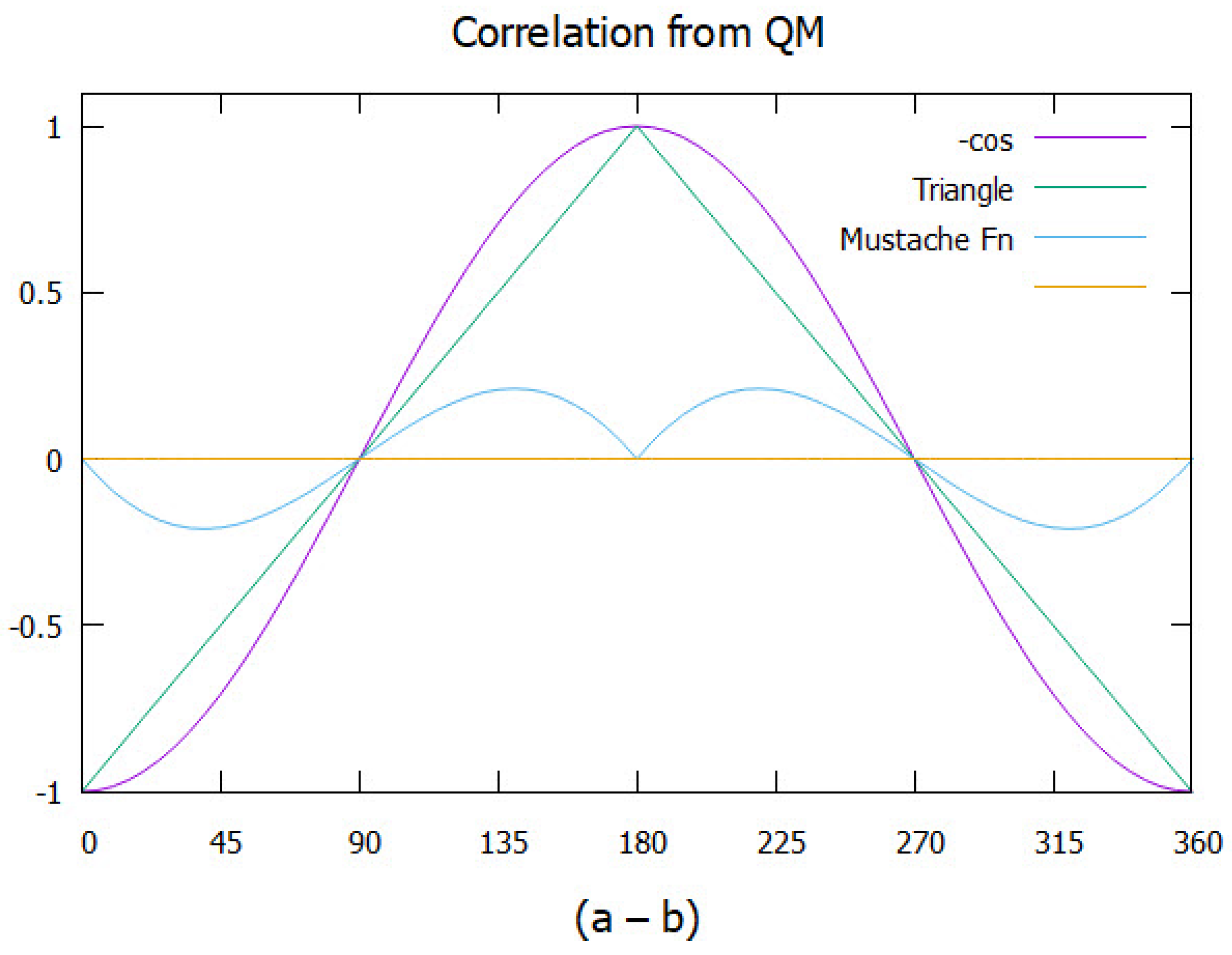
The correlation arising from an EPR pair, Eq.(3), has the well-known value of CHSH = giving the observed violation. This is plotted in Figure 2 versus . The product state given in Eq.(4), does not violate BI with a CHSH = 2. This is displayed in the figure as the triangle. Subtracting the two separates out the part that is responsible for the observed violation of BI, with CHSH = 0.828. We call this the mustache function. Bell’s theorem asserts this correlation can only arise from non-locality, or equivalently that no Local Variable (LV) model can account for the observed violation. In contrast, here we attribute the missing correlation to quantum coherence that was dropped upon particle separation under the assumption of locality.
In conclusion, if the quantum coherence terms are dropped when an EPR pair separates, the resulting product state does not agree with the experimental results. Including these terms is the purpose of this paper, and we show that they account for the full quantum correlation. That is, the violation is a result of coherence rather than non-local connectivity.
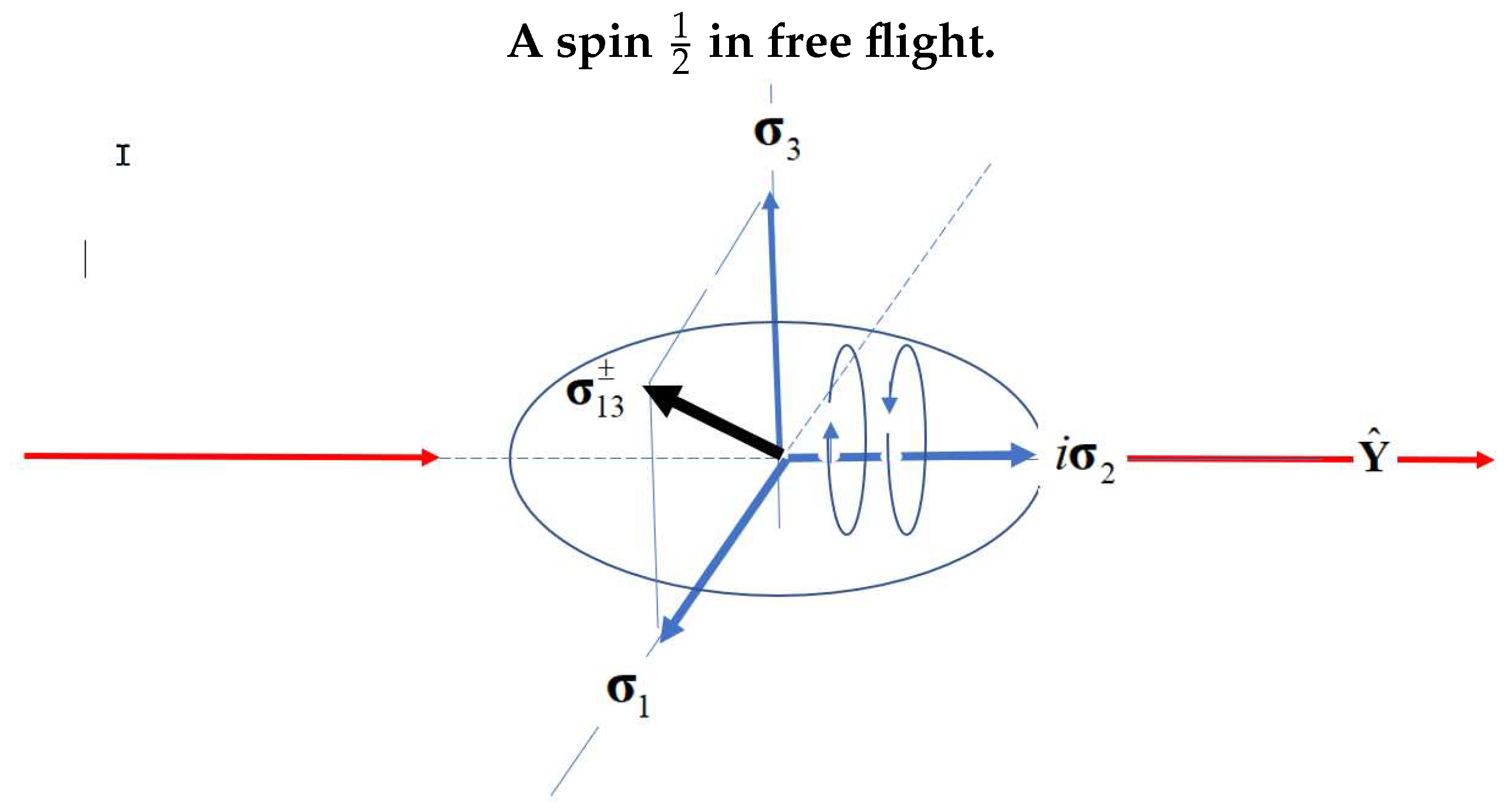
Figure 1.
Two properties of spin: its polarization perpendicular to its helicity. The helicity is in the direction of propagation and averages out the polarizations.
Figure 1.
Two properties of spin: its polarization perpendicular to its helicity. The helicity is in the direction of propagation and averages out the polarizations.
Geometric algebra
The calculation of Eqs.(3) and (4) involve the quantum trace over a dyadic, . One of the most fundamental equations from geometric algebra, [16] expresses a dyadic as the geometric product in terms of the symmetric scalar product and the anti-symmetric wedge product. This leads to the well-known relationship between spin components of
Note that this expression is complementary since the dyadic cannot be simultaneously symmetric and anti-symmetric (i cannot simultaneously be equal and not equal to j). Only one of the two can occur at any instant.
Although the coherent terms play no role in determining the observed spin polarization, they are still present. Polarization depends upon the difference between two measured spin states, . Here is a unit vector on the Bloch sphere. Motivated by Eq.(5), we defined the helicity, [6], as a complementary attribute to the polarization,
Using this anti-symmetric, anti-Hermitian second rank tensor operator in the same calculation as given above for the product states, Eq.(4), generates the missing correlation, [6],
Of course, added to the product of cosines in Eq.(4), this correlation fully accounts for the calculated in Eq.(3), suggesting the observe violation of BI is a result of helicity. Note also that the correlation from the two complementary parts, Eq.(4) and Eq.(7) is added. This is an example of the Conservation of Geometric Correlation, [6].
The Dirac equation
Here we summerize the results of reference, [7]. The Dirac equation provides the mathematical basis for spin. If helicity is an element of reality, it must be consistent with the Dirac equation. Just as Dirac interpreted his four dimensional field as consisting of a matter-antimatter pair of two states each, so should it also give a formal basis for the existence of helicity.
The Dirac field is represented by the gamma matrices, , involving time and the three spatial components. The Dirac equation contains no bivector so cannot describe the helicity. However, a bivector can be introduced by multiplying one gamma matrix by the imaginary number chosen to be . This is the only fundamental change introduced in the theory and the solution follows standard methods, [17].
Since Q-spin is structured, we define a BFF of which is a rotation away from the LFF, . Spin spacetime is .
As they must, the gamma matrices still anti-commute but the change to the Pauli spin components in the gamma matrices describes spin in terms of rather than . By multiplying by i, the usual spin symmetry of SU(2), is changed to being a normal subgroup of the quaternion group, . Whereas Dirac’s field is , the spin spacetime field becomes, . Introducing the bivector into the Dirac equation renders it non-Hermitian, [7]. It’s two solutions, , are mirror states analogous to Dirac’s matter-antimatter description.
Free particles exist in isotropy, whence the two spatial components, , are indistinguishable. Permuting them with a parity operator leaves them unchanged. In contrast the bivector is odd to parity, . This directly shows the two solutions are mirror states which reflect under parity, , and therefore have no definite parity, [7], themselves. These are the origin of the ± in the spin spacetime field.
However, the two mirror states can be combined to give states that are odd and even to parity, which leads immediately to the separation of spin spacetime, [7], into two distinct parts giving: a two dimension Dirac equation for the two spatial components; and a massless Weyl spinor equation for the bivector. The solution to the 2D Dirac equation is a plane, or disc, of spin angular momentum. The solution to the Weyl equation is a unit quaternion which spins the disc. The 2D spin states are even to parity while those of the quaternion space are odd to parity.
The quaternion version of the Dirac equation justifies the helicity as a real attribute of spin which is perpendicular to the 2D spin plane and co-linear to the LFF axis. Taking this as the axis of linear momentum, gives the view in Figure 1 with helicity spinning that axis. The two orthogonal spatial components, , are viewed as two spin axes, each carrying a magnetic moment . These are the mirror states. Also shown is the bisector of the two ferminoic axes, which depicts the boson. Notice that this structure is geometrically equivalent to that of a photon. The EPR pairs are in free flight from the source up until they encounter their filters.
In free flight only helicity is manifest since the spinning of the axis of linear momentum averages out the orthogonal resonance spin 1. The boson is still present on the particle, but suppressed as helicity dominates.
Upon encountering an anisotropic environment due to a polarizing field, the two spin axes, (3,1), are no longer indistinguishable and the mirror property is lost. This leads to the decoupling of Q-spin into its two polarized states of . We observe only one since the helicity is transferred to the aligned spin axis which causes its orthogonal twin to average to zero, Figure 3 (left and right panels). This recovers Dirac spin which obey’s Dirac’s equation and is the spin of that we measure. EPR coincidence experiments observe the transition from a boson in free-flight to a fermion upon measurement. How the resonant spin decouples depends upon the filter strength and its orientation relative to the resonant spin. This is discussed in the following section.
Two spin axes on the same particle is a different interpretation than given by Dirac, his being that the mirror states form a matter-antimatter pair.
Coherence and polarization are complementary properties of a spin.
Q-spin in a polarizing field
The complementary attributes of spin, polarization and coherence, simultaneously exist. However, only one is manifest at any instant. Just as a dyadic Eq.(5) is the sum of two complementary contributions, so we express Q-spin, , possessing both properties,
There are two of these, one for each axis, , , and they describe the disc which comes from the 2D Dirac equation. We combine these two axes, just like combining any angular momentum which constructively interfere to produce a purely resonance spin being a boson of magnitude 1,
The signs define the quadrants of the BFF. Since the results are the same for any quadrant, we use the first.
There are a number of expressions for this spin which we present without derivation, [7]. These show how the quaternions arise and govern the properties of a spin. The BFF is clearer than using the LFF, but eventually we must transform to the LFF where the experiments are done.
First, in the absence of a field, the expression for a single spin in free-flight is, (see [7] Eq.(10))
This shows each axis multiplied by a unit quaternion that rotates around the Y axis. The axis is rotated by , and axis is rotated by . Hence the two axes coincide and bisect the first quadrant and form the resonant boson spin, see Figure 4. By permuting the signs in Eq.(9), bisectors of all the quadrants are found, corresponding to the boson resonance spins. Of course, for a single Q-spin, only one of the quadrants carries a boson at any instant.
The transformation from the BFF to the LFF is given by,
In the presence of a field, the expectation value of the boson spin is
where the field is expressed in the LFF and oriented by angle
Contracting the field, Eq.(13), with Eq.(10), gives,
where the projections determine the contributions from each axis in the LFF,
This expression shows the competition between the two axes. In the absence of the vector field, the two axes are indistinguishable, but the field introduces asymmetry. Hence, one axis is closer to the field than the other, so the least action principle asserts it aligns while its partner spins orthogonal to it and averages out, see Figure 3 (left and right). The angles are given in the caption.
If or , then the field is aligned with the or axis respectively. Since the polarization from one axis is lost, the aligned axis has only of the polarization.
To get the full polarization, the resonance boson bisector must have , so the field is co-linear with the bisector and the polarization has magnitude of 1 due to equal contributions from and .
Choosing shows the field vector co-linear with the axis, orthogonal to with zero value.
If the field is co-linear with the boson spin, then it precesses without uncoupling. This is illustrated in the lower middle part of Figure 3, but as the field is oriented further from the bisector, the precession changes to nutation, wobbles and then decompose as the field strength increases and moves further from the resonance spin and closer to one of the fermionic axes. From Figure 4 the bisector lies 45° from either or axes. We therefore assume the boson decouples directly, without nutation, when the field axis lies greater than from the bisector. When, however, the field vector lies within from the boson, it precesses as a spin 1. Define a 45° wedge centered on the bisector, and within that cone, the boson spin remains intact until the field strength overpowers the spin-spin coupling, and it decouples.
Depending of these orientation effects, Q-spin either persists as a boson, or rapidly decouples to a fermion.
To find the expression where the bisectors are projected onto the LFF, use
which leads to, (see [7] Eq.(34))
Both axes of the BFF bivector are projected onto the LFF of Z and X respectively, and each is multiplied by a unit field quaternion. The magnitude of each term determines which axis aligns and which is averages out.
All the above can be expressed by a product of three quaternions, (see [7] Eq.(43)),
The first quaternion is a phase which is discussed above; the second is a geometric factor that orients the spin disc in the BFF; and the last is a field quaternion that sets the field position in the LFF.
Separating a EPR pair
Initially in a singlet state at the source, an EPR pair separates and the two independent particles move towards their respective filters. In the process they conserve linear momentum, angular momentum, and helicity, see Figure 5. The discs depict the separation process with the middle disc displaying the resonance spins of 1 which are anti-parallel for Alice and Bob at the source. Alice’s spin moves right and Bob’s moves left. Their initial orientation at the source is set by the angle . The axis of linear momentum spins with helicity being either left or right. Bob’s orientation is to conserve angular momentum. Both spin around the Y axis in the same direction, thereby maintaining them as anti-parallel in free flight.
Note that Alice and Bob are in opposite frames. Alice is in a right handed frame by the right hand rule, and Bob in the left. The two frames are related by complex conjugation, so that whereas they both have the same sense of precession, their helicities are opposite when Bob is viewed from a RH frame.
In the following we obtain the correlation from coincidence experiments in different cases.
Correlation from an EPR pair
In the absence of the filters, , the correlation is given by the product of the Q-spins for Alice and Bob,
The spins are anti-correlated at separation which requires differs between Alice and Bob by , see Figure 5. Also we have taken into account that the helicities of Alice and Bob’s spins are opposite, expressed by the complex conjugation. The second term reverses the helicity of both, so the correlation is real . As expected, after leaving a common source, in free-flight before encountering filters, the correlation between Alice and Bob is -1 consistent with the two spins remaining anti-parallel and anti-correlated from the source up to the filter.
Approaching a filter
As the spins of Alice and Bob approach their randomly set filters, the correlation between the two resonance states is
This is identical to the result that maintains entanglement as seen in Eq.(3). Using Q-spin the correlation is maintained by the common angle without any non-local connectivity between Alice and Bob. Note there is no contraction between the two spins because they have separated and no contraction is possible.
If one of the spins is polarized there is no helicity and only the scalar part of the quaternion is present,
and only the product state survives even if one spin is coherent,
If a spin is oriented with then , or if then and
To get the full correlation, Eq.(20), Alice and Bob’s particles must both be boson spins. Then the full correlation is obtained. If one or the other has decoupled into a fermion, only a product state is possible. That means the correlation from coherence can only be measured when the spins of both Alice and Bob are oriented within the same 45° wedge on either side of the anti-parallel boson spins. Within this wedge, as seen in Fig.(/reffig:CHSH), the boson axis, labeled with a 1, represents Alice and Bob’s anti-parallel bosons. Alice’s field axis
Interpretation of the CHSH inequality
Coupling of angular momentum is common in all spectroscopes [18], including transport properties of gases, [19,20]. In our case, the resonance spin is stable in free-flight but will eventually decouple as it approaches a filter. At a given distance, the decoupling depends upon the orientation of a spin relative to the filter; and its strength relative to the spin-spin coupling within Q-spin.
The violation of BI is expressed by the CHSH inequality, [1], which shows no classical system can exceed . EPR coincidence experiments, [1,2,3], violate this. Starting with a local singlet state at the source, the CHSH value of is found which exceeds 2. This is universally accepted as proof for non-locality, as Bell’s theorem asserts, [10].
Consider now, that the filter settings for both Alice and Bob are shown in Figure 6. Bob’s is one of and , and Alice’s settings is one of and a1 are shown, with = (d − c) and a1 =
(d + c). There are four experiments expressed in the CHSH inequality, whence Alice and Bob have settings of (−c, a3) , (d, a3), (d, a1), and (c, a1). We choose these setting because they give the maximum violation of the CHSH inequality.
The BFF for Alice and Bob coincide, and moreover, relative to the LFF, the BFF can take any orientation, (see Figure 4 and vary the angle between 0 and ). As the orientation of the BFF changes randomly, then the boson vector, will sample the filter with different ’s. Alice and Bob’s spins remain anti-parallel until they reach their filters, after which they start to feel a pull in opposite directions. In the cone, Alice is attracted to and Bob to , after which both precess about their field axis. This orientation ensures within the cone the bosons persists, and moving outside the cone, causes one to start to decouple. Alice and Bob stay within the cone of the time.
In summary, for fixed field settings, the boson’s will feel the field, and as long as a boson remain within the cone, Alice and Bob will align as bosons. Outside that setting, one axis, either Alice of Bob, will be beyond from its field, and will decompose to a fermion.
The maximum correlation for the S=CHSH inequality for the four experiments is determined by the filter setting as shown in Figure 6, giving,
Once aligned with a filter axis, Figure 7 shows Alice’s spin 1 precessing about filter direction, and Bob’s around his filter direction. This is consistent with Alice’s boson aligning with the field vector, intact, and the same for Bob at . As confirmation the bosons precesses intact, note a spin makes an angle of with the field direction. For a spin the angle is while a spin 1 has angle of 45°, thereby supporting the assertion that the boson is precessing in the field before decoupling, and is responsible for the violation, and not the fermion spin of .
We do not treat the dynamics of the 2D spin approaching the filter, but if the magnetic moment for each spin axis is , then the resonance spin of 1 has before it decouples and a Larmor frequency double that of the fermions with spin .
Simulation model
In contrast to a structureless point particle, Q-spin displays four internal motions with four axes. First the axis of linear momentum is spun by a quaternion. Next the two fermion axes can precess about their axes, or couple to give the fourth axis being the boson. In spin spacetime there are two dimensions, and . Additionally each axis carries helicity, Eq.(8), so each fernion axis also separates into a quaternion which spins the fermion axis. The coupled boson has no such quaternion. This gives 2 spatial dimensions in Minkowski space and dimensions from each hyper-sphere, for a total of 14 spatial dimensions associated with Q-spin. However, when the two fermions couple to a boson, one spatial dimension is lost since the boson is one dimensional.
The Q-spin structure then is due to the interaction between vectors, and the decoupling of a one dimensional boson into two fermions, each with one dimension. The coupled and uncoupled cases depend upon the angles shown in Eqs.(14) and (17). Either equation can be used, and Eq.(14) is simpler and is reproduced here,
We use the least action principle to determine the alignment and decoupling.
For polarization coincidences, either one of the two fermionic axis aligns, and we choose the real part of either axis above. Then we simply determine if it spins L (negative) or R (positive) giving a plus or minus click. This gives the triangle, Figure 8, and a CHSH value of 2. Specifically the simulation for polarizations uses either axis, .
and determines its sign.
The correlation from the bosons required that eventually it will decouple and become a fermion. Hence we first determine which of the two axes lies closer to the filter, and that axis aligns. Then we determine the sign of that axis as positive or negative giving + or − clicks. We write the two coupled boson axes as,
and then determine the larger axis as the one that will become polarized. We then determine its sign giving a + or − click.
Note that the field angle is doubled. This is because the coupled boson has twice the Larmor frequency compared with the fermion. Without this doubling, the simulation fails, again giving confirmation that the boson is present.
The boson correlation leads to the mustache function, and the coherence contribution from the coherence terms in Eq.(2). The CHSH value from coherence is 1. Specifically for coherence, first determine the larger axis,
and then uses that axis to determine the clicks.
Of course the same is done for Bob, and the coincidences from both Alice and Bob combine their clicks into equal coincidences or unequal coincidenes, .
The simulation determines the correlation between classical axes. It is not a quantum simulation, rather being a model that the treatment here suggests. Such classical simulations can account for the correlation without non-locality, [21], see also [22]. We note the total CHSH from polarization and coherence gives a total of CHSH=3, in contrast to that from an entangled state of .
Simulation results
The FORTRAN and C code, available with this paper, determines clicks from polarized states and coherent events using the above algorithms.
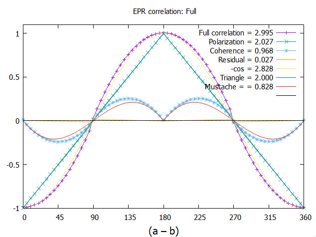
The results are given in Figure 8. The simulated correlation from either polarization axis gives the polarization as the triangle, with a CHSH = 2.027. The mustache coherence which depends on the coupling of the two axes into one axis, is shown in same figure and gives a CHSH = 0.968. That is, the simulation gives a total CHSH value of 2.995, or almost 3. The simulation gives more correlation than from quantum theory CHSH = 2.828.
Since polarization and coherence are complementary attributes, they are independent each contributing their correlation which is the sum of the two.
The theoretical CHSH value for polarizations is 2, whereas in Figure 8 it is 2.027. There is residual correlation that remains as shown in Figure 9. A cross over occurs close to the horizontal axis. It is hardly discernible. Considering it might be an artifact, various tests did not remove it. This has similar symmetry to the mustache coherence and supports this to be a real feature in the model. The are two discontinuities at and are necessary for the residue to be physical. We assert this residual contribution to coherence is due to correlation in the polarization states. If confirmed, the polarization exceeds BI, [9], by a small amount and violates his theorem [10].
Determining the correlation
Polarization and coherence are complementary properties which means that they are not manifest simultaneously [23,24]. Pauli stated [25] "Intuitively, observables are complementary if the experimental arrangements allowing their unambiguous definitions are mutually exclusive." In the case discussed here, the two complementary properties of polarization and coherence cannot yet be distinguished in EPR coincidence experiments. The origin of complementarity for spin is Eq.(5) which displays distinct properties which are symmetric and anti-symmetric, and therefore exclusive one from the other.
The correlation between equal coincidence events (), , and unequal events(), is given by
which gives the minus cosine similarity in EPR experiments.
Between these complementarity events there can be no mixed states since each exists in its own space and cannot belong to the same convex set. If they did, then a lever law mixing of two extreme points would apply, determined by the probabilities, and . However, with no mixed states, the probabilities are replaced by Boolean operators that ensure complementarity,
with or , with the sum of the contributions being the total number of events, .
Suppose that it is possible to filter the system such that the experiments can distinguish between the two, then we can write the total correlation as collecting the different events in different bins,
The correlation from each is evaluated to obtain the full correlation as shown in Figure 8 being the sum of the two contributions. Note the value of a correlation is independent of the total number of clicks, so for the calculation we did the following: first in Eq.(30) assume and and the polarization algorithm was used to give the triangle in Figure 8. Then we set and and calculated the mustache curve using the coherence algorithm.
We find that the correlation at the source from an entangled singlet, is divided between correlation from polarization and coherence. This is consistent with the conservation of geometric correlation, [6], which states that the total correlation at the source is conserved between EPR pairs upon separation.
A filter, in principle, might be constructed by polarizing the beam at the source for both Alice and Bob, adjust to be the same for all EPR pairs, and then arrange the filters at the desired angle relative to the polarized source. Such a pre-filter should distinguish between polarization and coherent states, allowing the coincidences to be sorted into bins, shown in Eq.(30), and then the corerlations evaluated.
Additionally, a filter might vary the strengths of the applied field to inhibit or promote decoupling
The mustache function
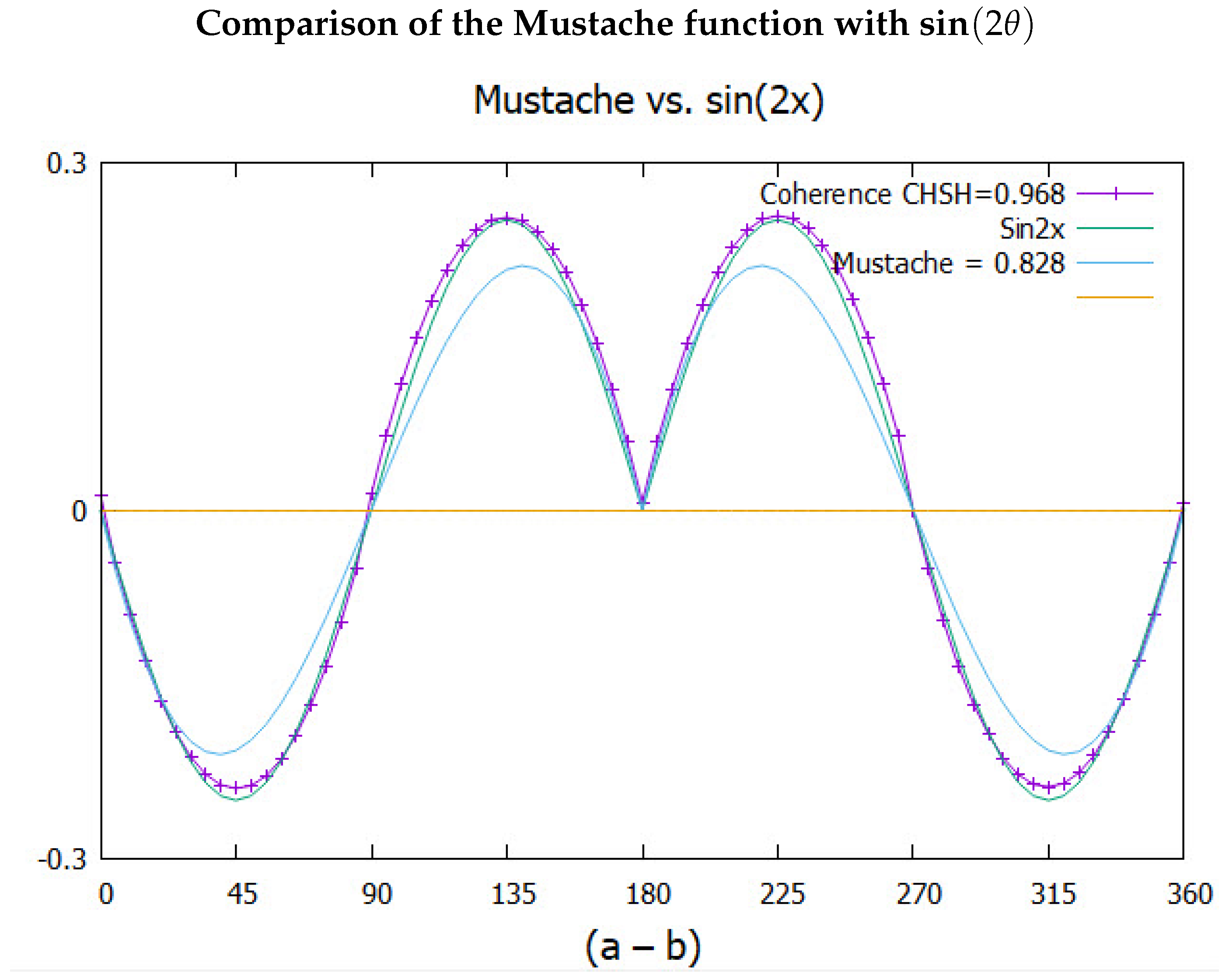
The coherence from the boson decoupling is responsible for the mustache, giving more correlation, but a similar structure, to the quantum correlation, see Figure 8. The Q-spin correlation , resembles two opposing sine waves which are reflected at . The following gives a good fit,
This is plotted in Figure 11 along with the simulated data points which match Eq.(31). Also plotted for comparison is the correlation from quantum theory. Note the filter angle is doubled, consistent with a magnetic moment of . Note also the prefactor of . Recall that of the time, the spins in the field are are bosons, and only of the coincidences contribute to the mustache, and to the polarization.
Figure 10.
The function given in Eq.(31) compared to the simulation. Also shown is the correlation from quantum theory.
Figure 10.
The function given in Eq.(31) compared to the simulation. Also shown is the correlation from quantum theory.
Discussion
We find the two complementary properties exist simultaneously. This supports Einstein in the famous Einstein-Bohr debates, [12]. However, only one property can be realized at any instant, thereby supporting Bohr’s notion of complementarity, [26]. Coherence and polarization are incompatible elements of reality. They influence each other. The spinor spins the polarization; the indistinguishably of the two polarization axes creates the parity for the helicity to know which way to spin.
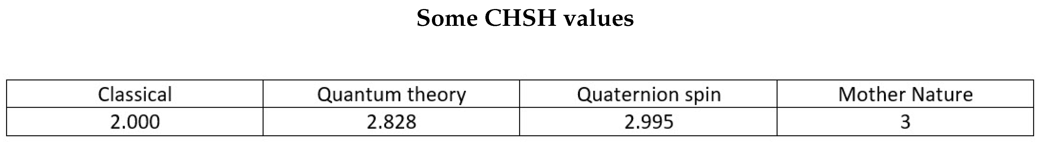
Figure 11 lists four values of the CHSH inequalities. The value of 2 quantifies the Invisible Boundary [27], between polarization and coherence. Quantum theory gives the value of which is less than that from the simulation of 2.995, which is close to 3. The value 3 is a result of modeling the three axes of Q-spin: the two polarized and one coherent, suggesting a CHSH = 1 for each axis.
The CHSH values leading to 2.995 from the simulation are and . This suggests a convergence to , which is correlation per axis. This leads to a CHSH value of 3 which supports equal contributions from each axis.
Spin
In this treatment, non-local entanglement is replaced by helicity. The Dirac spin is replaced with Q-spin. Both these features come from changing the symmetry from SU(2) to . The visualization of Q-spin, which is geometrically identical to that of a photon, see Figure 1, carries a 2D spin plane that forms its own “World Sheet”, [28]. The 2D structure of Q-spin admits anyons [29], consistent with a boson and a fermion on one particle. This is not possible in 3D or for a point particle.
When the Dirac equation is changed to include Q-spin, the two resulting mirror states are fundamental properties of Nature. They have no parity, only reflection, but they combine into states of even parity, polarization, and odd parity coherence.
Spin carries helicity as an element of reality, and quaternions exist in the hypersphere of four spatial dimensions. Spin extends to these spaces which are beyond our visualization, but nonetheless remains an element of reality beyond our dimension. The only part of a quaternion that is visible to us is the stereographic projection from onto our Minkowski spacetime. From that we can observe an axis spinning and we can account for the observed violation of BI.
According to the treatment here, however, EPR are validated in asserting that quantum theory is incomplete. Quantum mechanics is a theory of measurement but not of Nature. It does not include those higher dimensions of the hyper-sphere, needed for the coherence, nor does it include anti-Hermitian operators as elements of reality. Despite being contrary with the accepted philosophy, the treatment here gives an alternate and local realistic description of the microscopic.
In calculating expectation values, the state operator is given in reference ([6]), which includes both polarization axes. We do not include contributions from the helicity in the state operator because it is not physically observable in our spacetime. In the BFF, Q-spin is expressed by Eq.(10) with two axes, and projected along the field direction. The magnitude of those projections determine which axis is favoured to align, whereas if both axes are more or less equally projected, being in a wedge, then the resonance spin of magnitude 1 is favoured.
To repeat, in free-flight Q-spin acts like a boson and in a perturbing field, it acts like a fermion.
Bell
The CHSH form of Bell’s inequalities provides a quantitative measure of correlation, and enables us to separate classical (polarization) from quantum (helicity) correlation. Bell’s theorem is distinct from his inequalities and asserts in Bell’s words [10],
If [a hidden-variable theory] is local it will not agree with quantum mechanics, and if it agrees with quantum mechanics it will not be local.
Although this is an incorrect interpretation by Bell regarding the violation of his inequalities, the mathematics of his theorem is not disputed. The question arises as to how Q-spin can account for the observed correlation without non-local connectivity which directly contradicts the theorem.
Bell assumed only classical correlation in deriving his inequalities. He neglected the complementary property, whereby a spin has two distinct elements of reality, each of which contributes to the correlation in different ways. In agreement with Einstein, [4] both complementary properties exist on a particle at the same instant. Filters cannot presently distinguish between the two but if they could, then the complementary property should be evident.
In short, in his classical treatment, Bell assumes that Nature is described by observables belonging to one convex set. A quantum system can have several distinct convex sets which describe incompatible components of a system. In our case there is one for polarization another for coherence.
We have found that the violation of Bell’s Inequalities is a result of an additional source of correlation by a complementary attribute of the system.
In this work, there are no hidden variables. Nonetheless, we find a CHSH value of 2 for polarization and 1 for coherence, neither of which violates Bell’s theorem. The theorem is misleading, pointing to non-locality as the consequence of the violation, whereas here it is due to the decoupling of the resonance spin. Bell’s theorem states that classical events cannot exceed a CHSH of 2. Simply stated, Bell’s Theorem is not applicable to quantum systems. The stark conclusion is that non-locality, which is universally accepted, is replaced by this local treatment that leads to the conclusion that the observed violation is evidence for local realism and not non-locality, [30].
We do not criticize local entanglement and only assert that non-local entanglement is untenable. We view local entanglement as an essential property of quantum theory. Indeed we concur with who famously stated, [31], that entanglement was not “a” but “the” difference from classical. However, we can show that an entangled singlet state is an approximaiton. For this reason, the quantum correlation of is less than the simulated value of CHSH=3. Entanglement is a fundamental property of quantum theory but not of Nature. It simplifies calculations by dropping coherent terms, and the price is missing correlation and structure.
Note, however, that the simulated CHSH = 2.027 for polarization shows that a local realistic theory can violate BI. It arises from canceled terms in forming the singlet approximation.
Conclusions
The existence of Q-spin requires accepting that Nature has reality beyond our spacetime; that there is information lost; [32], and there are properties in Nature we cannot observe. Some limitations of quantum mechanics can be addressed by replacing Dirac spin with Q-spin, and entanglement with helicity.
In the vast majority of cases of interest, spin is not in free flight but is polarized in bonds. Q-spin, however, if accepted, changes our fundamental view of Nature, and requires re-examination of areas of quantum theory that have hitherto relied on non-local connectivity, [1,2,3,33] to [37].
The violation of Bell’s inequalities is not evidence for non-locality, a difficult concept to grasp, but rather evidence for the existence of helicity and other properties of Nature that are responsible for local realism.
Acknowledgments
The author is grateful to Pierre Leroy, (programmer) and Chantal Roth, PhD (programmer) for their help and patience with simulation methods. I thank Pierre who converted the FORTRAN Program to C.
References
- Clauser, J. F., Horne, M. A., Shimony, A., Holt, R. A. (1969). Proposed experiment to test local hidden-variable theories. Physical review letters, 23(15), 880. [CrossRef]
- Aspect, Alain, Jean Dalibard, and Gérard Roger. “Experimental test of Bell’s inequalities using time-varying analyzers.” Physical review letters 49.25 (1982): 1804. Aspect, Alain (15 October 1976). “Proposed experiment to test the non separability of quantum mechanics”. Physical Review D. 14 (8): 1944–1951. [CrossRef]
- Weihs, G., Jennewein, T., Simon, C., Weinfurter, H., Zeilinger, A. (1998). Violation of Bell’s inequality under strict Einstein locality conditions. Physical Review Letters, 81(23), 5039. [CrossRef]
- Einstein, Albert, Boris Podolsky, and Nathan Rosen. “Can quantum-mechanical description of physical reality be considered complete?.” Physical review 47.10 (1935): 777. [CrossRef]
- Greenberger, D. M., Horne, M. A., Shimony, A., Zeilinger, A. (1990). Bell’s theorem without inequalities. American Journal of Physics, 58(12), 1131-1143. [CrossRef]
- Sanctuary, B. Spin with helicity.. Preprints 2023, 2023010571. [CrossRef]
- Sanctuary, B. Extrinsic Quaternion Spin. Preprints.org 2023, 2023020055. [Google Scholar] [CrossRef]
- Dirac, P. A. M. (1928). The quantum theory of the electron. Proceedings of the Royal Society of London. Series A, Containing Papers of a Mathematical and Physical Character, 117(778), 610-624. [CrossRef]
- Bell, John S. “On the Einstein Podolsky Rosen paradox.” Physics Physique Fizika 1.3 (1964): 195.
- Bell, J. S. “Speakable and Unspeakable in Quantum Mechanics” (Cambridge University Press, 1987), 2004. See “Locality in quantum mechanics: reply to critics. Epistemological Letters”, Nov. 1975, pp 2–6.”.
- Fano, Ugo. “Description of states in quantum mechanics by density matrix and operator techniques.” Reviews of modern physics 29.1 (1957): 74. [CrossRef]
- Jammer, M. (1974). Philosophy of Quantum Mechanics. the interpretations of quantum mechanics in historical perspective.
- Newton to Bentley, 25 February 1692/3, The Correspondence of Isaac Newton, ed. H. W. Turnbull (Cambridge: Cambridge University Press, 1961).
- Einstein, Albert. Born-Einstein Letters 1916-1955: Friendship, Politics and Physics in Uncertain Times. Palgrave Macmillan, 2014.
- Mullin, W. J. (2017). Quantum weirdness. Oxford University Press.
- Doran, C., Lasenby, J., (2003). Geometric algebra for physicists. Cambridge University Press. [CrossRef]
- Peskin, M. E., Schroeder, D. V. (1995). An Introduction To Quantum Field Theory (Frontiers in Physics), Boulder, CO.
- Herzberg, Gerhard. Molecular Spectra and molecular structure-Vol I. Vol. 1. Read Books Ltd, 2013.
- Turfa, A. F., Connor, J. N. L., Thijsse, B. J., Beenakker, J. J. M. (1985). A classical dynamics study of Senftleben-Beenakker effects in nitrogen gas. Physica A: Statistical Mechanics and its Applications, 129(3), 439-454. [CrossRef]
- Sanctuary, B. C., J. J. M. Beenakker, and J. A. R. Coope. "Influence of nuclear spin couplings on the thermomagnetic torque in HD." The Journal of Chemical Physics 60.8 (1974): 3352-3353. [CrossRef]
- Arto Annila, Marten Wikstrom, 2021, viXra:2112.0118 Quantum Entanglement: Bell’s Inequality Trivially Violated Also Classically. Category: Quantum Physics Quantum entanglement and classical correlation have the same form Arto Annila and Marten Wikstr.
- Geurdes, H. (2023) Bell’s Theorem and Einstein’s Worry about Quantum Mechanics. Journal of Quantum Information Science, 13, 131-137. [CrossRef]
- Kiukas, J., Lahti, P., Pellonpää, JP. et al. Complementary Observables in Quantum Mechanics. Found Phys 49, 506–531 (2019). [CrossRef]
- Busch, P., Grabowski, M., Lahti, P.: Operational Quantum Physics, LNP 31. Springer, New York, 1994, 2nd Corrected Printing (1997).
- Dirac, Paul Adrien Maurice. The principles of quantum mechanics. No. 27. Oxford university press, 1981.
- Bohr, Niels. "Can quantum-mechanical description of physical reality be considered complete?." Physical review 48.8 (1935): 696. [CrossRef]
- Wick, David. “The Infamous Boundary: Seven decades of heresy in quantum physics.” Springer Science and Business Media, 2012.
- Maldacena, J.; Susskind, L. Cool horizons for entangled black holes. Fortschritte der Physik 2013, 61, 781–811. [Google Scholar] [CrossRef]
- Wilczek, F. (1982). Quantum mechanics of fractional-spin particles. Physical review letters, 49(14), 957. [CrossRef]
- Abellán, Carlos, et al. Challenging local realism with human choices. arXiv preprint 2018. arXiv:1805.04431.
- Schrödinger E., “Discussion of probability relations between separated systems”. Mathematical Proceedings of the Cambridge Philosophical Society. 31 (4): 555–563 (1935). [CrossRef]
- Braunstein, Samuel L., and Arun K. Pati. “Quantum information cannot be completely hidden in correlations: implications for the black-hole information paradox.” Physical review letters 98.8 (2007): 080502. [CrossRef]
- Bennett, C. H., Brassard, G., Crépeau, C., Jozsa, R., Peres, A., Wootters, W. K. (1993). Teleporting an unknown quantum state via dual classical and Einstein-Podolsky-Rosen channels. Physical review letters, 70(13), 1895. [CrossRef]
- Kim, Y. H., Yu, R., Kulik, S. P., Shih, Y., Scully, M. O. (2000). Delayed “choice” quantum eraser. Physical Review Letters, 84(1), 1. [CrossRef]
- Van Raamsdonk, M. (2010). Building up spacetime with quantum entanglement. General Relativity and Gravitation, 42(10), 2323-2329. [CrossRef]
- Bashar, M. A., Chowdhury,M. A., Islam, R., Rahman, M. S., and Das,S. K. , “A Review and Prospects of Quantum Teleportation," 2009 International Conference on Computer and Automation Engineering, 2009, pp. 213-217. [CrossRef]
- Gisin, N., Ribordy, G., Tittel, W., Zbinden, H., Quantum cryptography. Reviews of modern physics, 74(1), 145, 2002. [CrossRef]
Figure 3.
The longer arrow denotes the direction of the polarizing field. The two polarization axes form Q-spin of even parity from the coupling of two mirror states. (middle top), The two mirror states in free flight, and couple to give the boson spin 1. (left and right) The axis closer to the field axis aligns. (middle lower) When the boson spin is close to the field, it precesses as a spin 1 before decoupling into its fermion components.
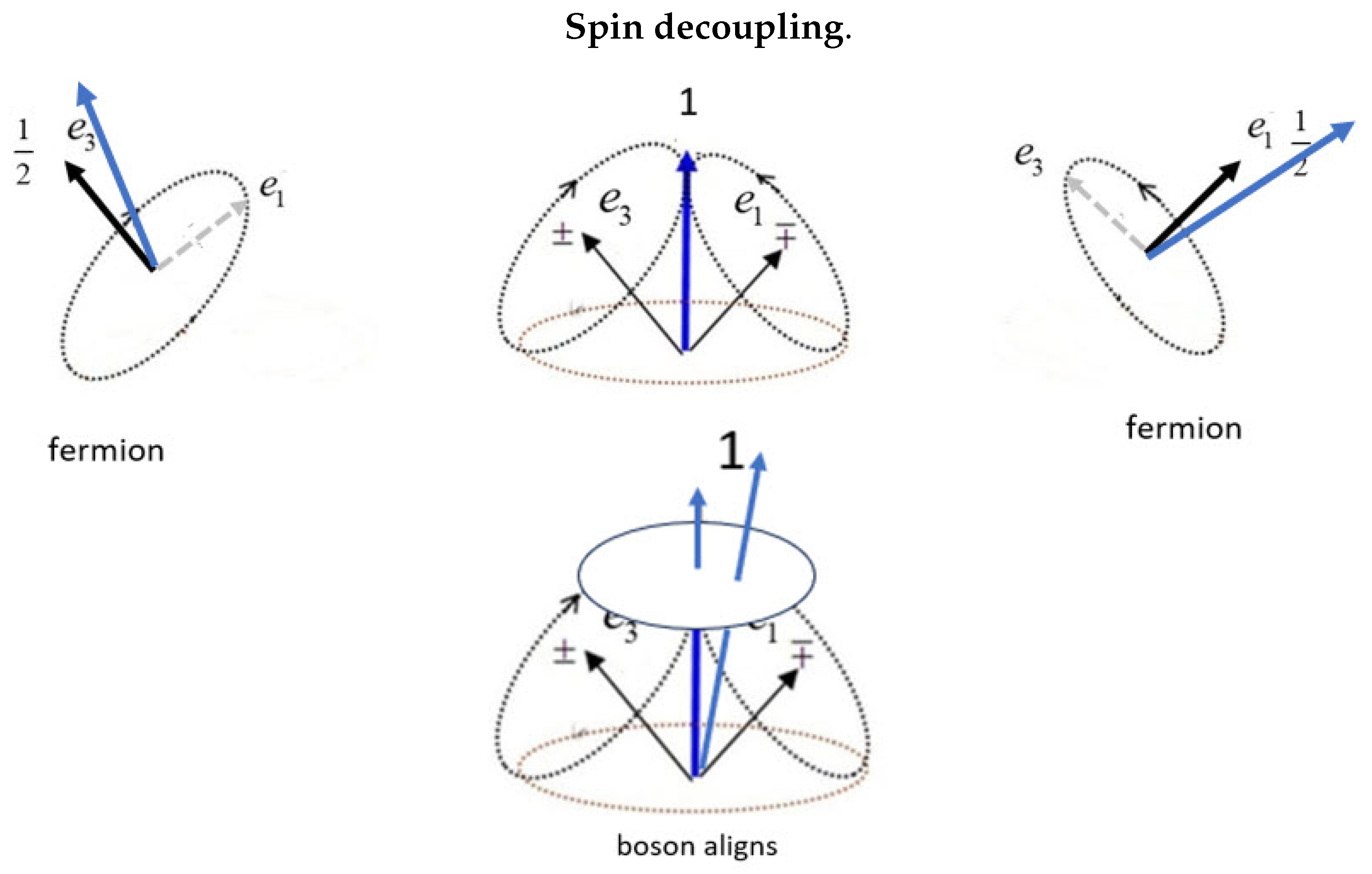
Figure 4.
The BFF showing the plane and the bisectors of the quadrants with boson spins of 1. The boson is labeled. The plane is oriented in the LFF by the Z axis, and the angle is shown. Also orients the field vector in the LFF. The angle is the orientation of a spin vector on the Bloch sphere.
Figure 4.
The BFF showing the plane and the bisectors of the quadrants with boson spins of 1. The boson is labeled. The plane is oriented in the LFF by the Z axis, and the angle is shown. Also orients the field vector in the LFF. The angle is the orientation of a spin vector on the Bloch sphere.
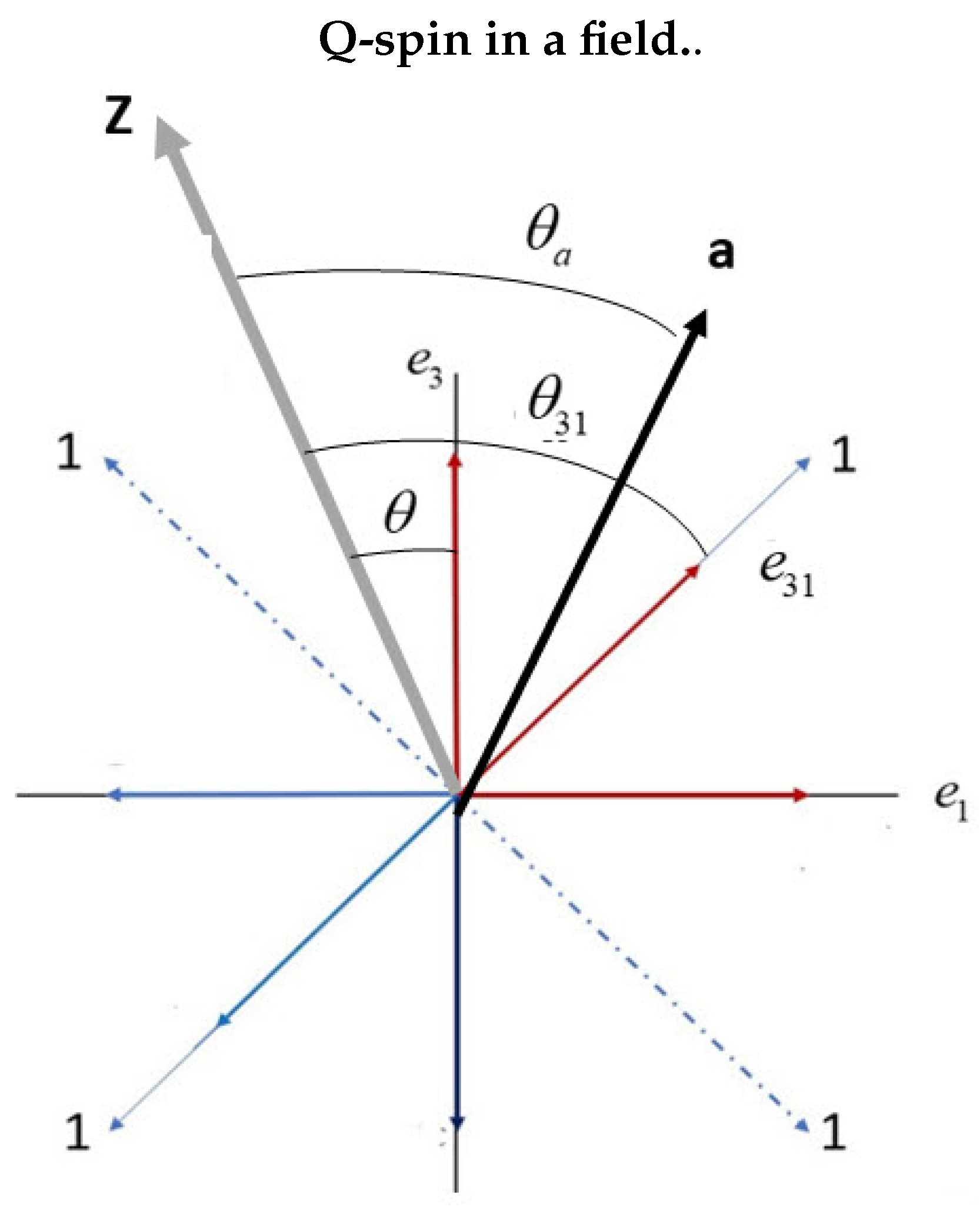
Figure 5.
Alice goes right in a RH coordinate frame and Bob goes left in a LH frame. The two spins precess in the same direction, either clockwise or anti-clockwise. Changing Bob’s frame from L to R means the helicity of the two particles is opposite. Note in the center figure that Alice and Bob start off with the same but opposite orientation in the BFF indicated by .
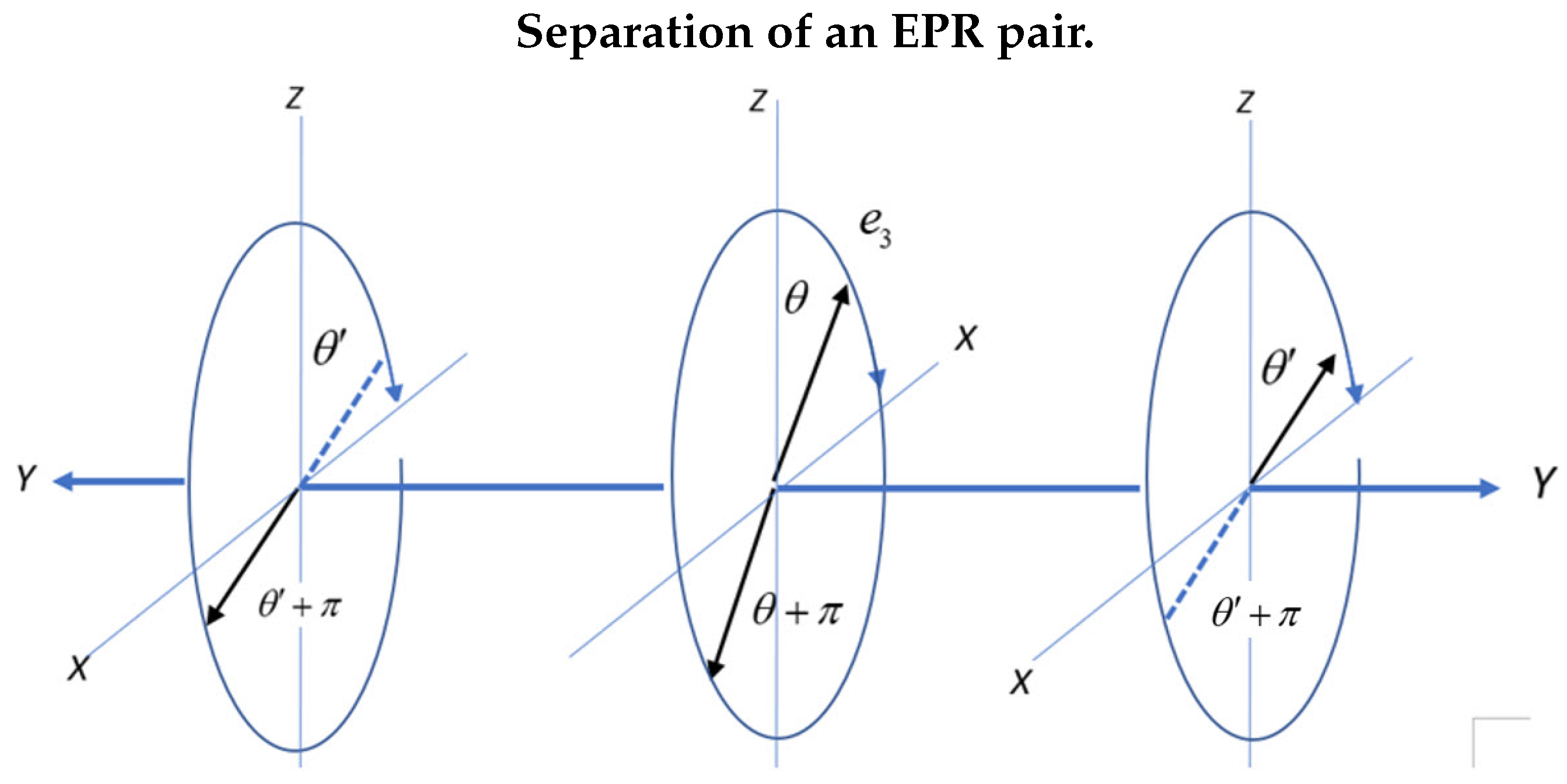
Figure 6.
Showing both Alice and Bob’s spins by looking along the axis of linear momentum, orthogonal to the screen. Within the two 45° wedges both Alice and Bob’s spins are bosons. The heavy lines are possible filter settings, such that if one axis is Alice’s filter setting, the adjacent setting is Bob’s and so on alternating from Alice and Bob.
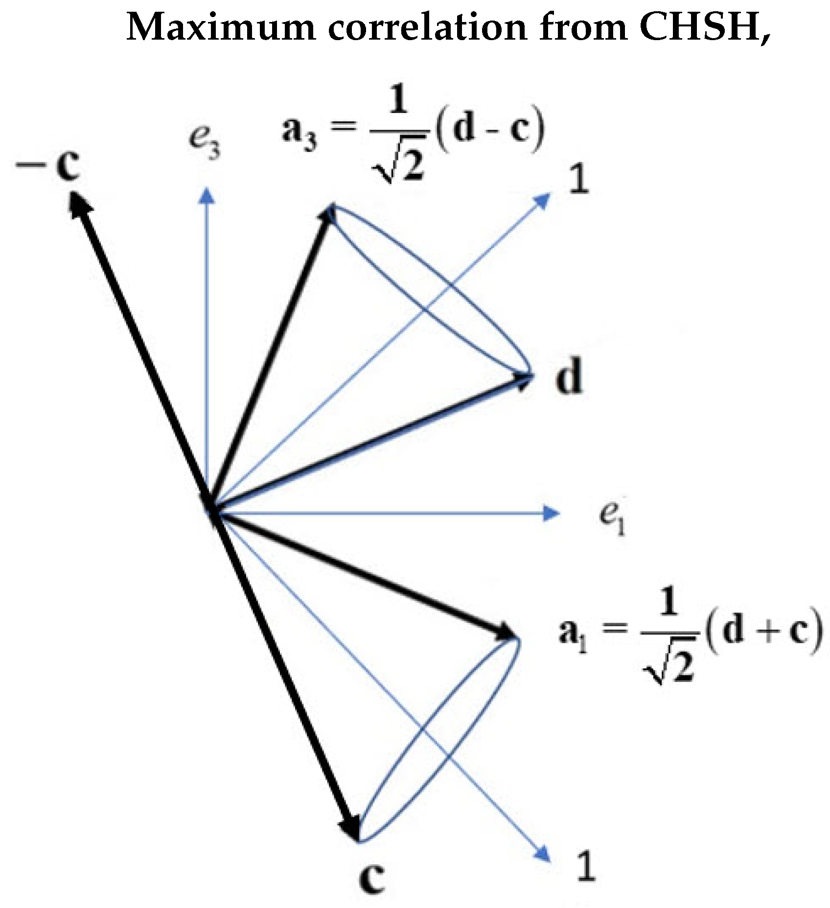
Figure 7.
Displaying the maximum correlation from coherence. Alice sets her filter to and the boson spin of 1 aligns. Bob has two settings that will give the maximum violation by applying his filter either along d or along at 45° from . Alternately, Alice can set her filter angle to and Bob has two filter settings, d and c that lead to the maximum correlation. Note that a spin of magnitude 1 makes an angle of 45° with filter directions.
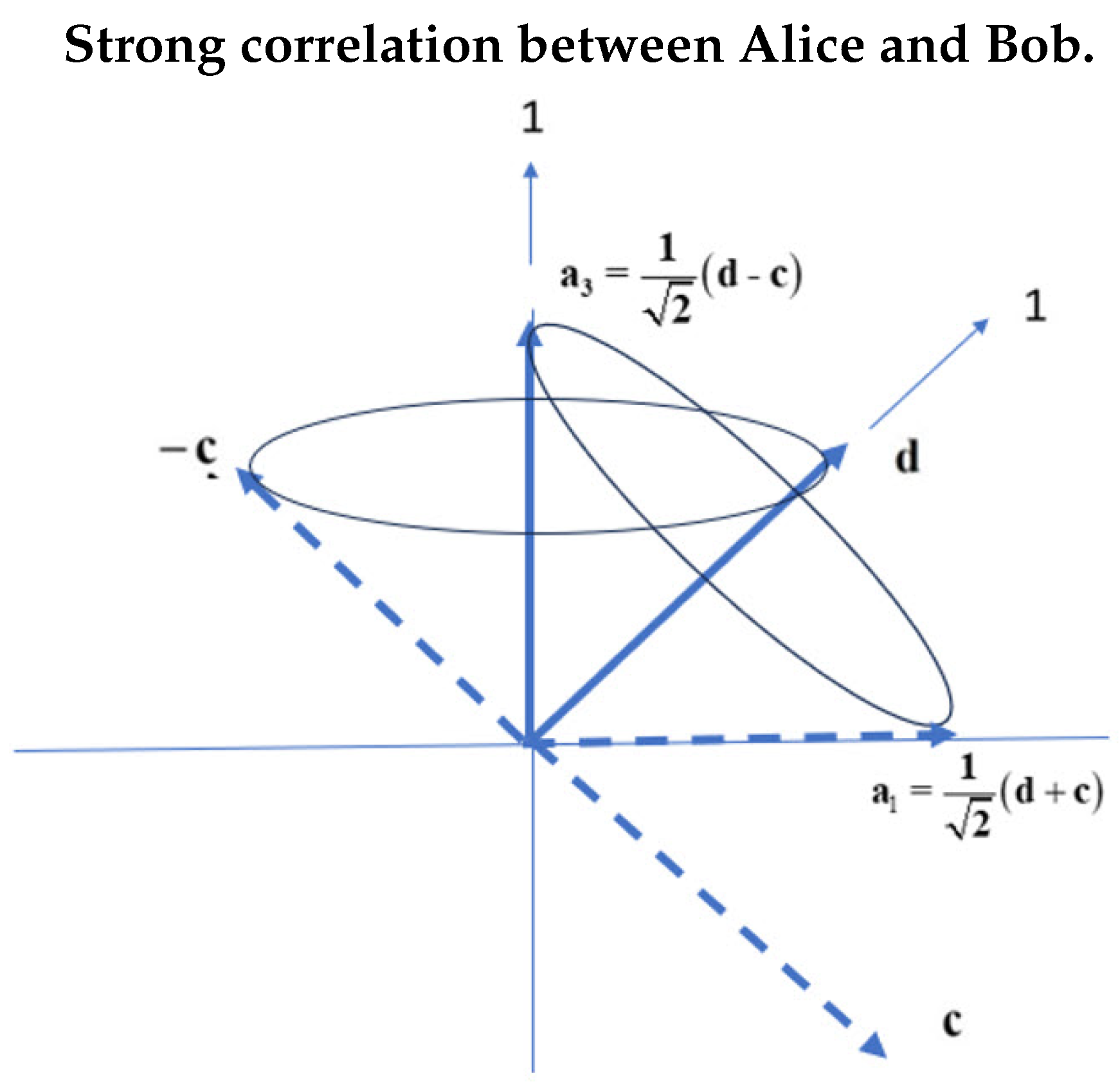
Figure 8.
Plotting intensity versus the angle difference The results of the simulation are given by the blue points. The CHSH values are listed. The full correlation is the sum of that from polarization, the triangle, and coherence, the mustache. Note the hardly discernible residual quaternion correlation along the horizontal axis.
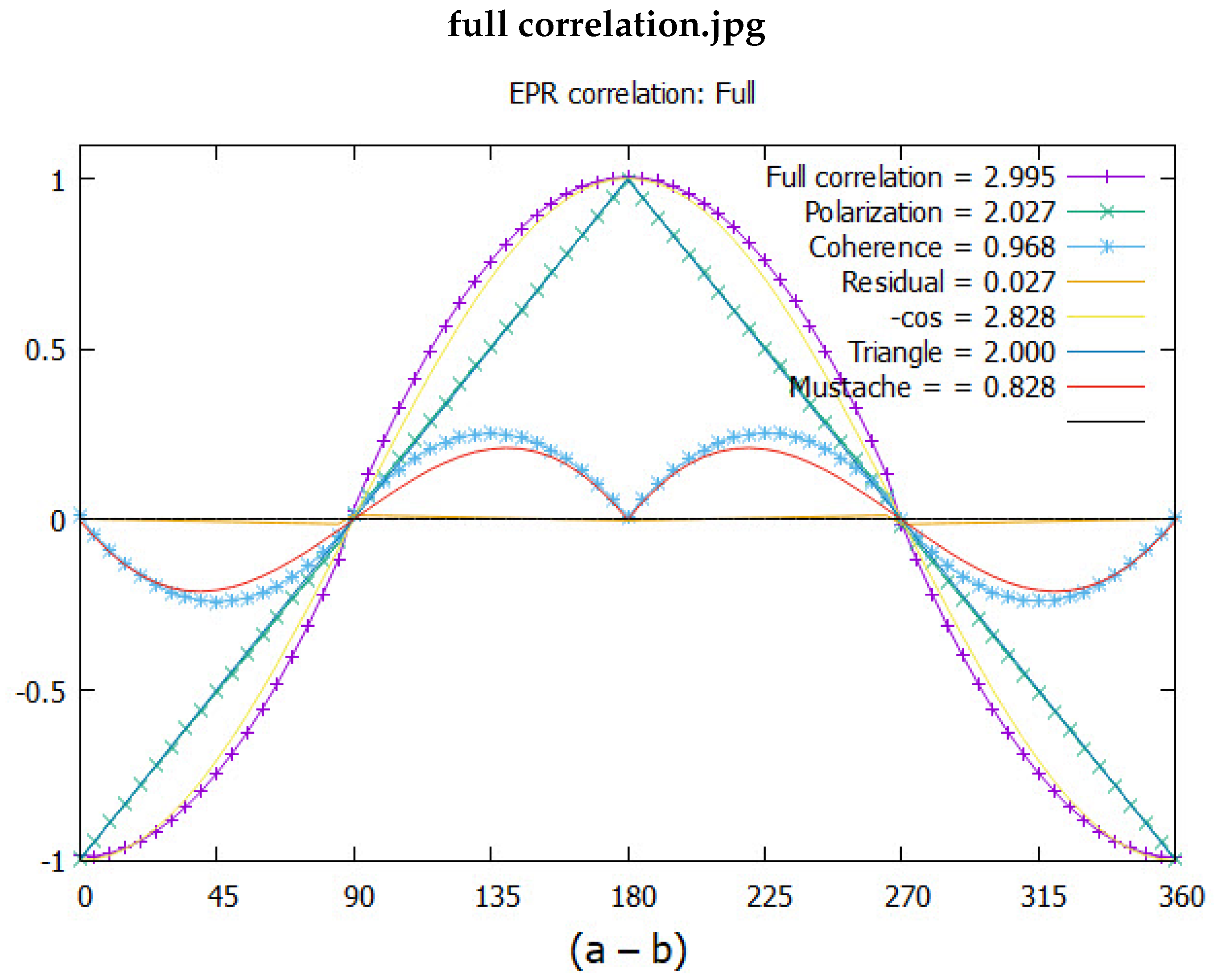
Figure 9.
A blow up of the simulated polarization compared to an exact triangle. The insert shows it over 2.
Figure 9.
A blow up of the simulated polarization compared to an exact triangle. The insert shows it over 2.
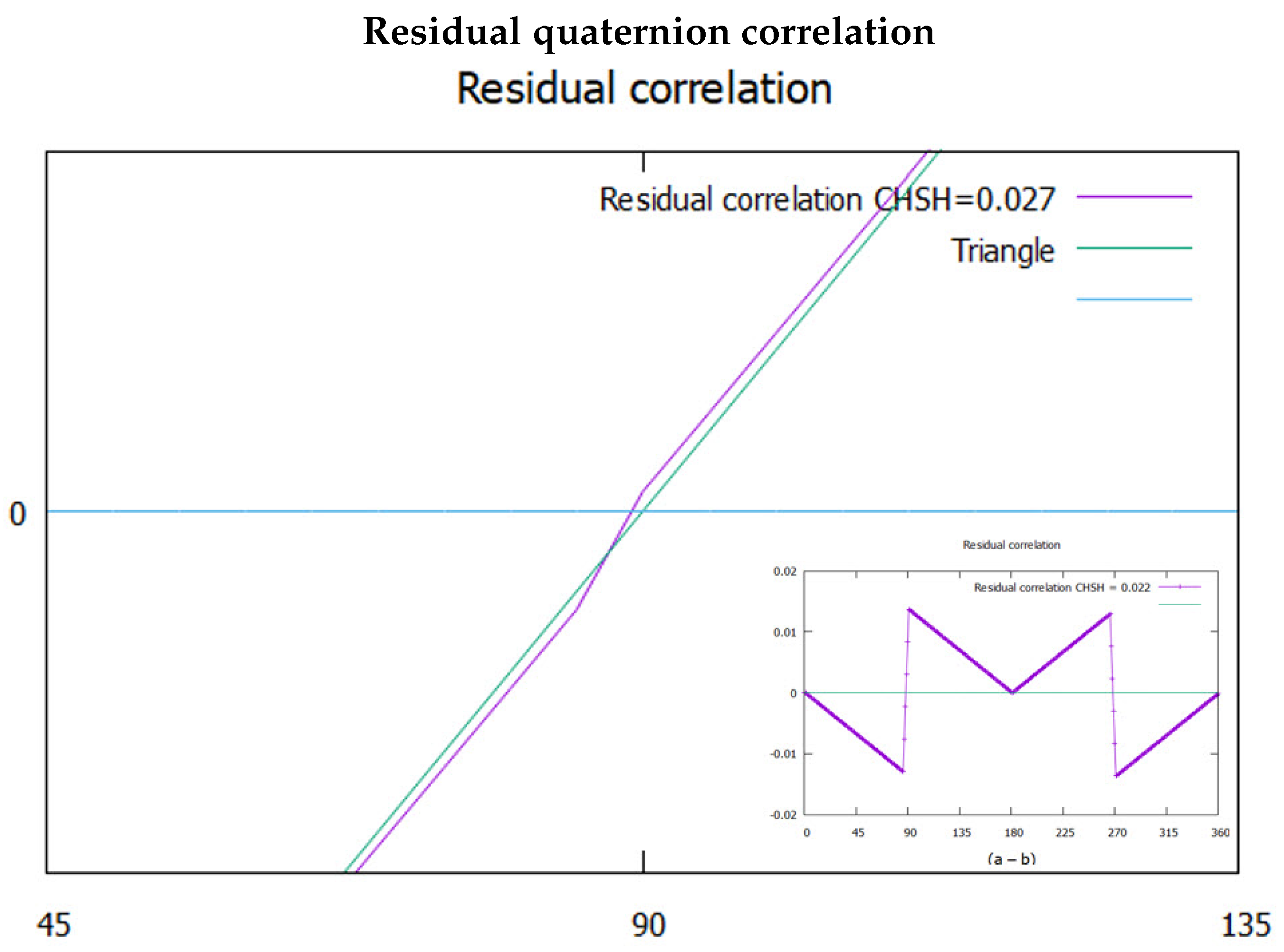
Figure 11.
Values of the CHSH inequalities from classical to Nature.
Disclaimer/Publisher’s Note: The statements, opinions and data contained in all publications are solely those of the individual author(s) and contributor(s) and not of MDPI and/or the editor(s). MDPI and/or the editor(s) disclaim responsibility for any injury to people or property resulting from any ideas, methods, instructions or products referred to in the content. |
© 2024 by the authors. Licensee MDPI, Basel, Switzerland. This article is an open access article distributed under the terms and conditions of the Creative Commons Attribution (CC BY) license (http://creativecommons.org/licenses/by/4.0/).
Copyright: This open access article is published under a Creative Commons CC BY 4.0 license, which permit the free download, distribution, and reuse, provided that the author and preprint are cited in any reuse.


