Submitted:
23 January 2023
Posted:
31 January 2023
You are already at the latest version
Abstract
Keywords:
1. Introduction
2. Materials and Methods
3. Results
4. Wind Power Generation
5. Conclusions
Author Contributions
Funding
Data Availability Statement
Acknowledgments
Conflicts of Interest
References
- Himri Y, Rehman S, Draoui B, Himri S. Wind power potential assessment for three locations in Algeria. Renewable and Sustainable Energy Reviews 2008; 12:2495 – 2504. [CrossRef]
- Thomas, L. Ackera, Susan K. Williamsb, Earl P.N. Duquea, Grant Brummels, Jason Buechler. Wind resource assessment in the state of Arizona: Inventory, capacity factor, and cost. Renewable Energy 2007; 32:1453–1466. [CrossRef]
- Laerte de Araujo Lima, Celso Rosendo Bezerra Filho. Wind energy assessment and wind farm simulation in Triunfo - Pernambuco, Brazil. Renewable Energy 2010; 35: 2705-2713. [CrossRef]
- Meishen Li, Xianguo Li. Investigation of wind characteristics and assessment of wind energy potential for Waterloo region, Canada. Energy Conversion and Management 2005; 46: 3014–3033. [CrossRef]
- Adrian Ilinca, Ed McCarthy, Jean-Louis Chaumel, Jean-Louis Re´tiveau. Wind potential assessment of Quebec Province. Renewable Energy 2003; 28: 1881–1897. [CrossRef]
- Zhou Y, Wu W X, Liu G X. Assessment of Onshore Wind Energy Resource and Wind-Generated Electricity Potential in Jiangsu, China. Energy Procedia 2011; 5: 418–422. [CrossRef]
- Ahmed Shata A S, Hanitsch R. Electricity generation and wind potential assessment at Hurghada, Egypt. Renewable Energy 2008; 33: 141–148. [CrossRef]
- Ahmed Shata Ahmed. Wind energy as a potential generation source at Ras Benas, Egypt. Renewable and Sustainable Energy Reviews 2010; 14: 2167–2173. [CrossRef]
- Getachew Bekele, Björn Palm. Wind energy potential assessment at four typical locations in Ethiopia. Applied Energy 2009; 86: 388–396. [CrossRef]
- Ravita D Prasad, Bansal R C, Sauturaga M. Wind Energy Analysis for Vadravadra Site in Fiji Islands: A Case Study. IEEE TRANSACTIONS ON ENERGY CONVERSION 2009; 24: 750-757. [CrossRef]
- Ioannis Fyrippis, Petros J. Axaopoulos, Gregoris Panayiotou. Wind energy potential assessment in Naxos Island, Greece. Applied Energy 2010; 87: 577–586. [CrossRef]
- Vogiatzis N, Kotti K, Spanomitsios S, Stoukides M. Analysis of wind potential and characteristics in North Aegean, Greece. Renewable Energy 2004; 29: 1193–1208. [CrossRef]
- Lin Lu, Hongxing Yang, John Burnett. Investigation on wind power potential on Hong Kong islands—an analysis of wind power and wind turbine characteristics. Renewable Energy 2002; 27: 1–12. [CrossRef]
- Daoo V J, Panchal N. S, Faby S, Sitaraman V, Krlshnamoorthy T. M. Assessment of wind energy potential of Trombay, Mumbai (19.18N; 72.88E), India. Energy Convers 1998; 13: 1351-1356. [CrossRef]
- Mirhosseini M, Sharifi F, Sedaghat A. Assessing the wind energy potential locations in province of Semnan in Iran. Renewable and Sustainable Energy Reviews 2011; 15: 449–459. [CrossRef]
- Mostafaeipour, A. Feasibility study of harnessing wind energy for turbine installation in province of Yazd in Iran. Renewable and Sustainable Energy Reviews 2010; 14: 93–111. [CrossRef]
- Mostafaeipour A, Sedaghat A, Dehghan-Niri A A, Kalantar V. Wind energy feasibility study for city of Shahrbabak in Iran. Renewable and Sustainable Energy Reviews 2011; 15: 2545–2556. [CrossRef]
- Keyhani A, Ghasemi-Varnamkhasti M, Khanali M, Abbaszadeh R. An assessment of wind energy potential as a power generation source in the capital of Iran, Tehran. Energy 2010; 35: 188–201. [CrossRef]
- Ouammi A, Dagdougui H, Sacile R, Abdelaziz M. Monthly and seasonal assessment of wind energy characteristics at four monitored locations in Liguria region (Italy). Renewable and Sustainable Energy Reviews 2010; 14: 1959–1968. [CrossRef]
- Bivona S, Burlon R, Leone C. Hourly wind speed analysis in Sicily. Renewable Energy 2003; 28:1371–1385. [CrossRef]
- Alghoul M A, Sulaiman M Y, Azmi B Z, and Wahab M Adb. Wind Energy Potential of Jordan. International Energy Journal 2007; 8: 71-78.
- Kamau J N, Kinyua R, Gathua J K. 6 years of wind data for Marsabit, Kenya average over 14 m/s at 100 m hub height; An analysis of the wind energy potential. Renewable Energy 2010; 35: 1298–1302. [CrossRef]
- [23] Islam M R, Saidur R, Rahim N A. Assessment of wind energy potentiality at Kudat and Labuan, Malaysia using Weibull distribution function. Energy 2011; 36: 985 – 992. [CrossRef]
- Muzathik A M, Wan Nik W B, Ibrahim M Z, Samo K B. Wind Resource Investigation of Terengganu in the West Malaysia. Wind Engineering 2009; 33: 389–402. [CrossRef]
- Mpholo M, Mathaba T, Letuma M. Wind profile assessment at Masitise and Sani in Lesotho for potential off-grid electricity generation. Energy Conversion and Management 2012; 53: 118–127. [CrossRef]
- Jaramillo O A, Borja M A. Bimodal versus Weibull Wind Speed Distributions: An Analysis of Wind Energy Potential in La Venta, Mexico. Wind Engineering 2004; 28: 225–234.
- Jaramillo O A, Saldan R, Miranda U. Wind power potential of Baja California Sur, Mexico. Renewable Energy 2004; 29: 2087–2100. [CrossRef]
- Jaramillo O A, Borja M A. Wind speed analysis in La Ventosa, Mexico: a bimodal probability distribution case. Renewable Energy 2004; 29: 1613–1630. [CrossRef]
- Fagbenle R O, Katende J, Ajayi O O, Okeniyi J O. Assessment of wind energy potential of two sites in North-East, Nigeria. Renewable Energy 2011; 36: 1277-1283. [CrossRef]
- Ohunakin O S, Adaramola M S, Oyewola O M. Wind energy evaluation for electricity generation using WECS in seven selected locations in Nigeria. Applied Energy 2011; 88: 3197–3206. [CrossRef]
- Adaramola M S, Paul S S, Oyedepo S O. Assessment of electricity generation and energy cost of wind energy conversion systems in north-central Nigeria. Energy Conversion and Management 2011; 52: 3363–3368. [CrossRef]
- Ohunakin OS, Akinnawonu OO. Assessment of wind energy potential and the economics of wind power generation in Jos, Plateau State, Nigeria. Energy for Sustainable Development 2012; 16: 78–83. [CrossRef]
- AL-Yahyai S, Charabi Y, Gastli A, Al-Alawi S. Assessment of wind energy potential locations in Oman using data from existing weather stations. Renewable and Sustainable Energy Reviews 2010; 14: 1428–1436. [CrossRef]
- Ullah I, Chaudhry Q, Chipperfield A J. An evaluation of wind energy potential at Kati Bandar, Pakistan. Renewable and Sustainable Energy Reviews 2010; 14: 856–861. [CrossRef]
- Safari, B. Modeling wind speed and wind power distributions in Rwanda. Renewable and Sustainable Energy Reviews 2011; 15: 925–935. [CrossRef]
- Cabello M, Orza J A G. Wind speed analysis in the province of Alicante, Spain. Potential for small-scale wind turbines. Renewable and Sustainable Energy Reviews 2010; 14: 3185–3191. [CrossRef]
- Carta J A, Ramı´rez P, Vela´zquez S. A review of wind speed probability distributions used in wind energy analysis Case studies in the Canary Islands. Renewable and Sustainable Energy Reviews 2009; 13: 933–955. [CrossRef]
- Abdeen M, O. On the wind energy resources of Sudan. Renewable and Sustainable Energy Reviews 2008; 12: 2117–2139. [CrossRef]
- Tsang-Jung Chang, Yu-Ting Wu, Hua-Yi Hsu, Chia-Ren Chu, Chun-Min Liao. Assessment of wind characteristics and wind turbine characteristics in Taiwan. Renewable Energy 2003; 28: 851–871. [CrossRef]
- Dahmouni A W, Ben Salah M, Askri F, Kerkeni C, Ben Nasrallah S. Assessment of wind energy potential and optimal electricity generation in Borj-Cedria, Tunisia. Renewable and Sustainable Energy Reviews 2011; 15:815–820. [CrossRef]
- Ali, N. Celik. Review of Turkey’s current energy status: A case study for wind energy potential of Canakkale province. Renewable and Sustainable Energy Reviews 2011; 15: 2743– 2749. [CrossRef]
- Onat N, Ersoz S. Analysis of wind climate and wind energy potential of regions in Turkey. Energy 2011; 36: 148-156. [CrossRef]
- Eskin N, Artar H, Tolun S. Wind energy potential of Gokceada Island in Turkey. Renewable and Sustainable Energy Reviews 2008; 12: 839–851. [CrossRef]
- Ucar A, Balo F. Evaluation of wind energy potential and electricity generation at six locations in Turkey. Applied Energy 2009; 86: 1864–1872. [CrossRef]
- Ozgurm A, Arslan O, Kose R, Peker K O. Statistical Evaluation of Wind Characteristics in Kutahya, Turkey. Energy Sources 2009; 31:1450–1463. [CrossRef]
- Arslan, O. Technoeconomic analysis of electricity generation from wind energy in Kutahya, Turkey. Energy 2010; 35:120–131. [CrossRef]
- Nguyen, KQ. Wind energy in Vietnam: Resource assessment, development status and future implications. Energy Policy 2007; 35:1405–1413. [CrossRef]
- Tran VT, Chen TH. Assessing the wind energy for rural areas of Vietnam. International Journal of Renewable Energy Research 2013; 3:423 – 528.
- "GWEC, Global Wind Report Annual Market Update". Gwec.net. http://www.gwec.net/index.php?id=180. Retrieved 2011-05-14.
- "EWEA - European Wind Energy Association". https://www.ewea.org/index.php?id=1487. Retrieved 2011-05-14.
- Israel Ministry of Environmental Protection, “Renewable Energy”. https://www.sviva.gov.il. Retrieved 2014-07-31.
- "Wind energy power generation", Background paper written by Orli Lotan, 21.09.05. Knesset, Research and Information Center, Jerusalem, 2005, p. 3 (in Hebrew).
- Ditkovich Y, Kuperman A, Yahalom A, and Byalsky M. A generalized approach to estimating capacity factor of fixed speed wind turbines. IEEE Transactions on Sustainable Energy 2013; 3:607 – 608. [CrossRef]
- Ditkovich Y, Kuperman A, Yahalom A, Byalsky M. Site-dependent wind turbine performance index. International Journal of Renewable Energy Research 2013; 3:592 – 594.
- Ditkovich Y, Kuperman A. Comparison of three methods for wind turbine capacity factor estimation. The Scientific World Journal 2014; 805238: 1 – 7. [CrossRef]
- Chang, TP. Performance comparison of six numerical methods in estimating Weibull parameters for wind energy application. Applied Energy 2011; 88:272-282. [CrossRef]
- Masters, G. Renewable and efficient electric power systems. John Wiley & Sons, New York, 2004.
- Kuperman A, Rabinovici R, Weiss G. Torque, and power limitations of a shunt connected inverter based WECS. WSEAS Transactions on Circuits and Systems 2005; 7:684 – 690.
- Kuperman A, Rabinovici R, Weiss G. A shunt connected inverter based variable speed wind turbine generation. International Journal of Electromotion 2006; 13:67-72.
- Gualtieri G, Secci S. Extrapolating wind speed series vs. Weibull distribution to assess wind resource to the turbine hub height: A case study on coastal location in Southern Italy. Renewable Energy 2014; 62:164-176. [CrossRef]
- Gualtieri G, Secci S. Methods to extrapolate wind resource to the turbine hub height based on power law: A 1-h wind speed vs. Weibull distribution extrapolation comparison. Renewable Energy 2013; 43:183-200. [CrossRef]
- Sergei Kolesnik, Moshe Sitbon, Asher Yahalom & Alon Kuperman "Assessment of Wind Resource Statistics in Samaria Region" Proceedings of the 16th International Scientific Conference on Engineering for Rural Development, P. 1409-1416, 24-26.05.2017. Jelgava, Latvia.
- Hasmat Malik, Nuzhat Fatema, Atif Iqbal, Chapter 8 - Intelligent Data Analytics for Wind Speed Forecasting for Wind Power Production Using Long Short-Term Memory (LSTM) Network, Editor(s): Hasmat Malik, Nuzhat Fatema, Atif Iqbal, Intelligent Data-Analytics for Condition Monitoring, Academic Press, 2021, Pages 165-192, ISBN 9780323855105. [CrossRef]
- Panagiotis Triantafyllou, John K. Kaldellis, 2.16 - Wind Power Industry and Markets, Editor(s): Trevor M. Letcher, Comprehensive Renewable Energy (Second Edition), Elsevier, 2022, Pages 497-566, ISBN 9780128197349. [CrossRef]
- John, K. Kaldellis, 2.01 - Introduction to Wind Energy, Editor(s): Trevor M. Letcher, Comprehensive Renewable Energy (Second Edition), Elsevier, 2022, Pages 1-12, ISBN 9780128197349. [CrossRef]
- Carrillo, C.; Obando Montaño, A.F.; Cidrás, J.; Díaz-Dorado, E. Review of power curve modelling for wind turbines. Renew. Sustain. Energy Rev. 2013, 21, 572–581. Available online: http://grupo_ene.webs.uvigo.es/ (accessed on 17 September 2015). [CrossRef]
- Doron Greenberg, Michael Byalsky & Asher Yahalom “Valuation of Wind Energy Turbines Using Volatility of Wind and Price” Electronics 2021, 10, 1098. [CrossRef]

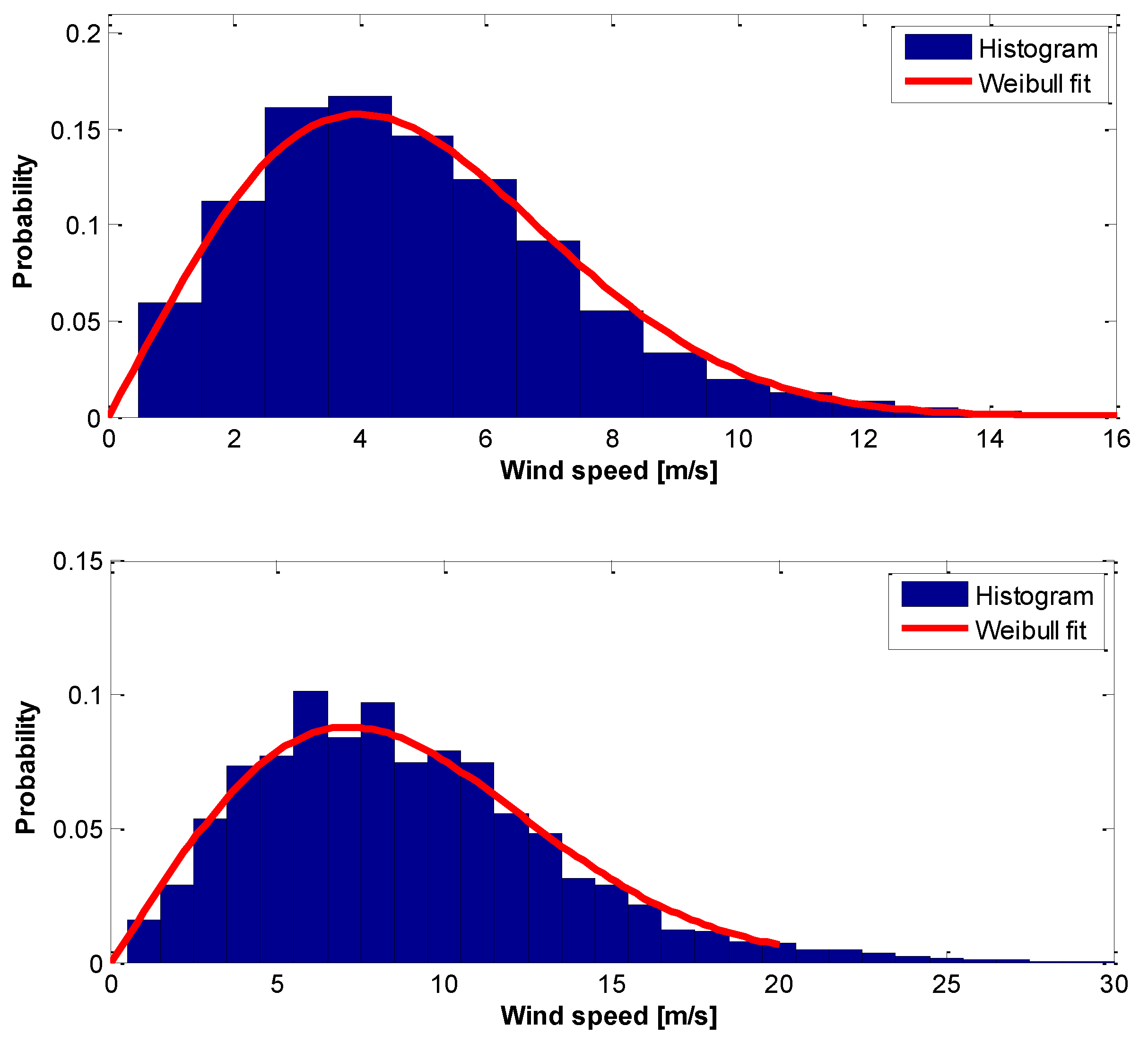
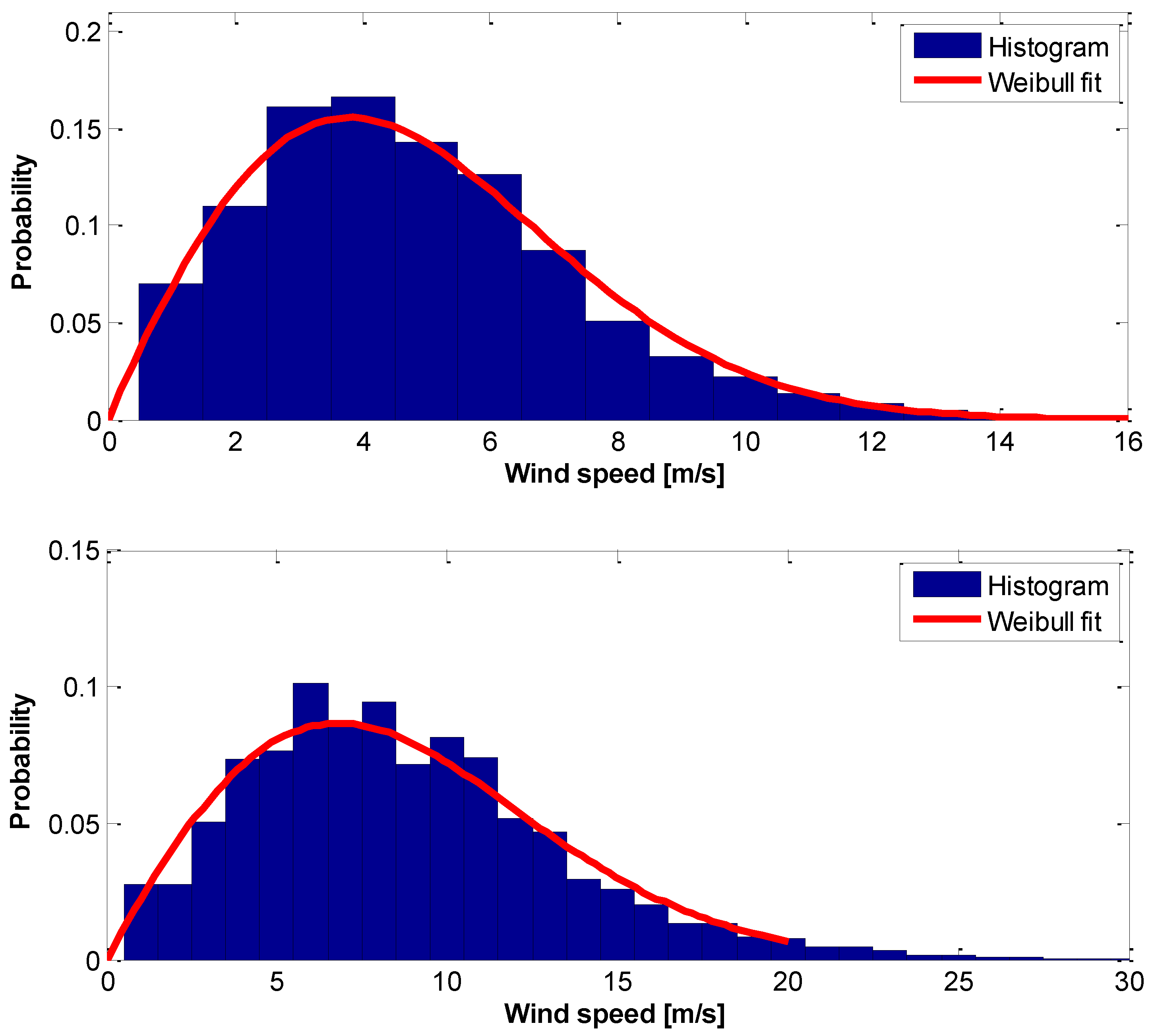
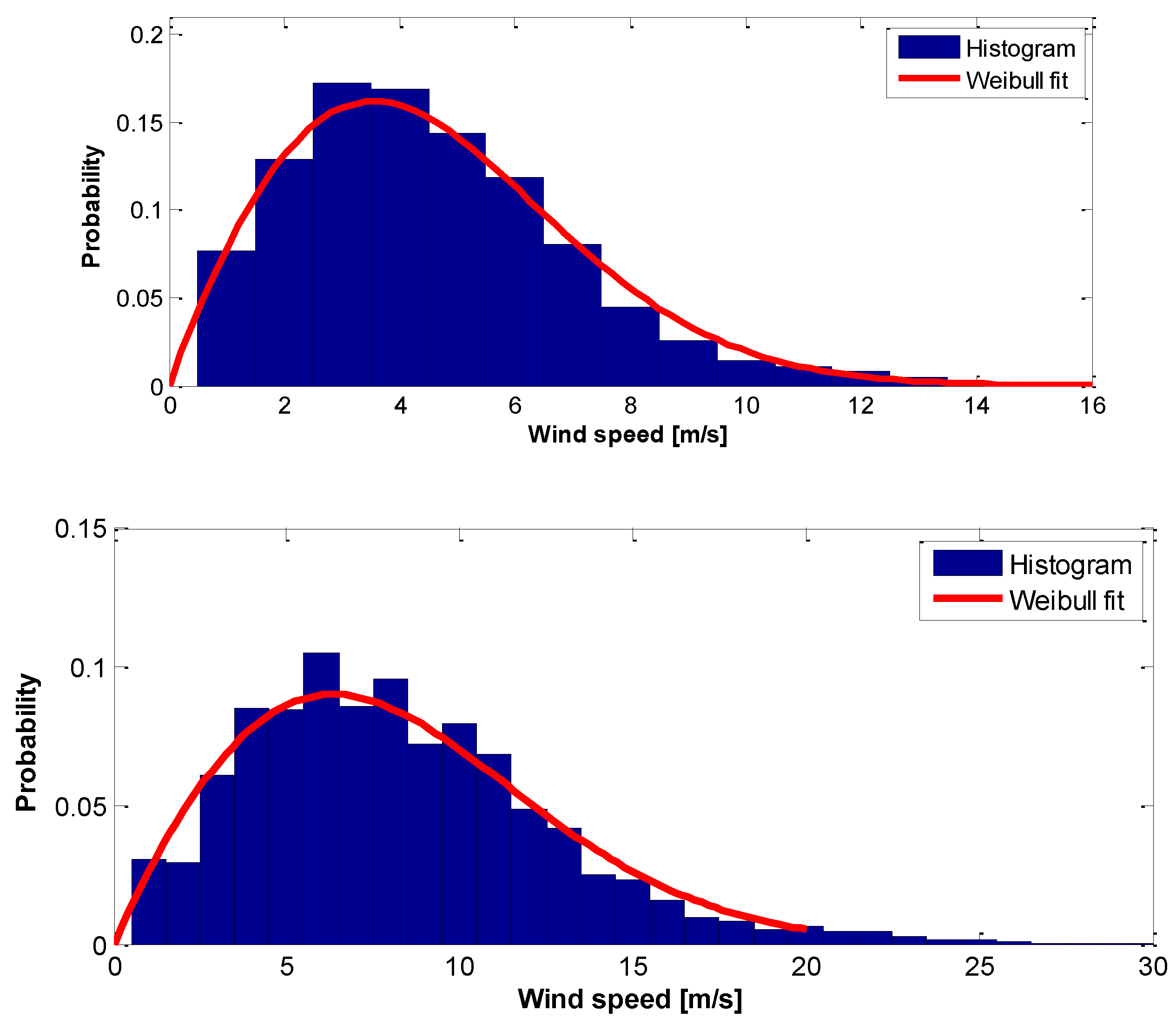
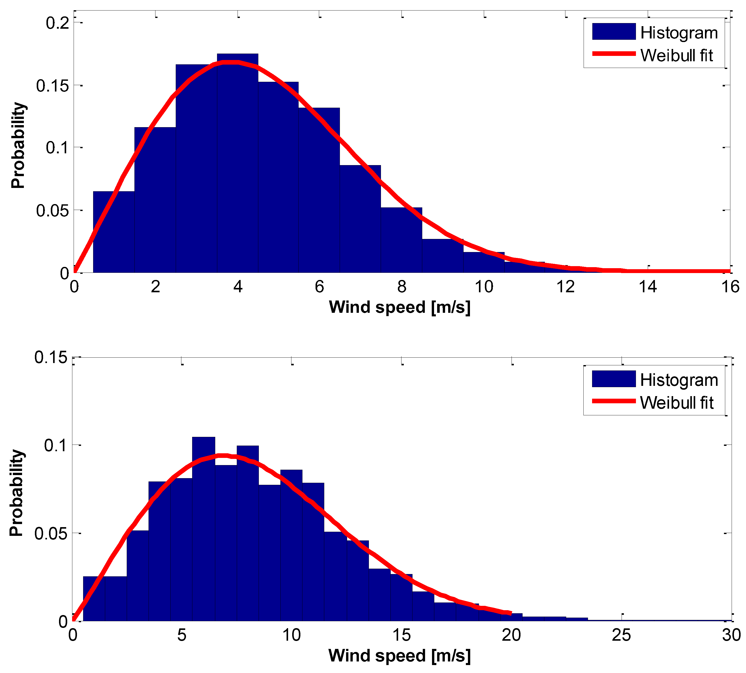

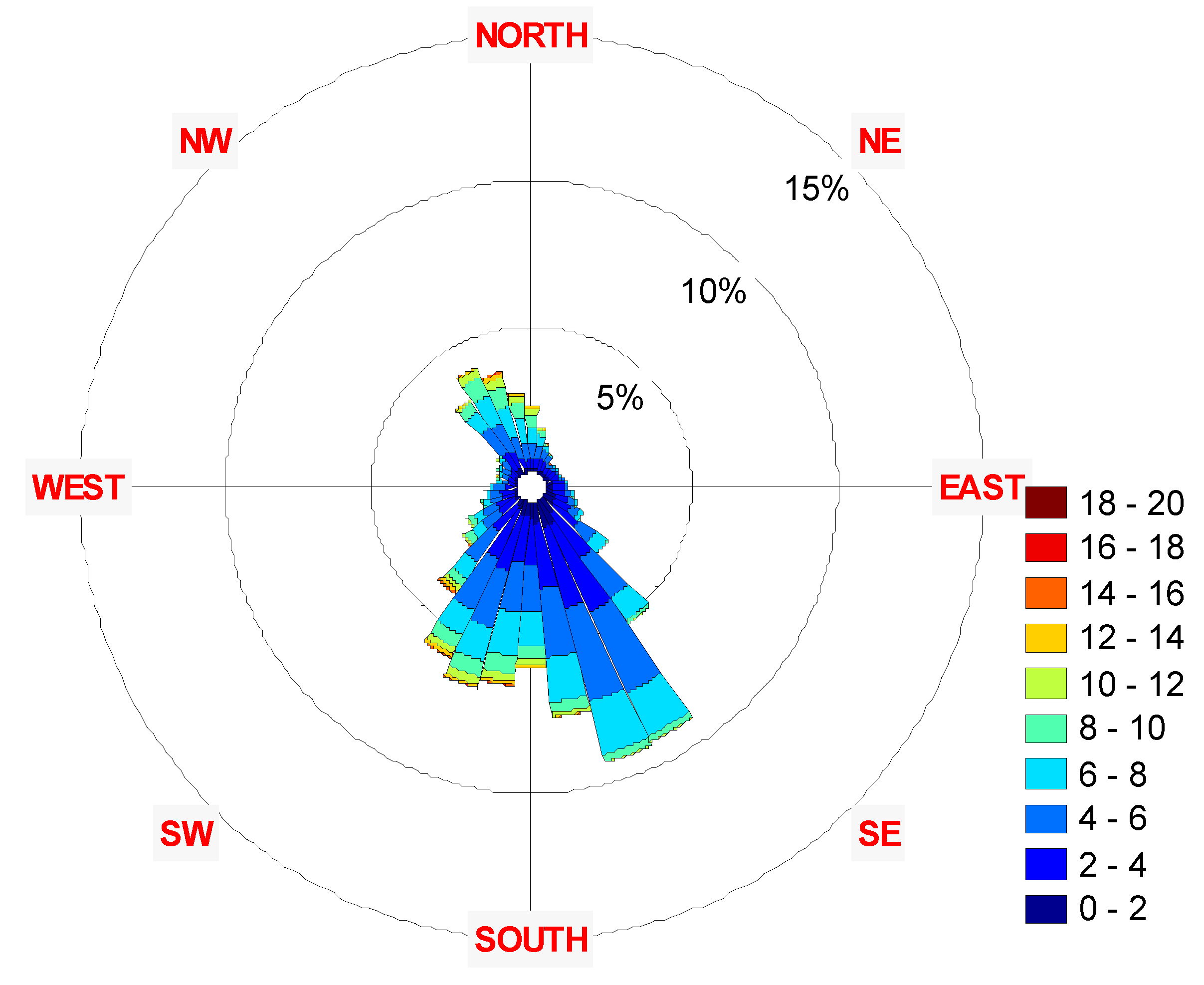
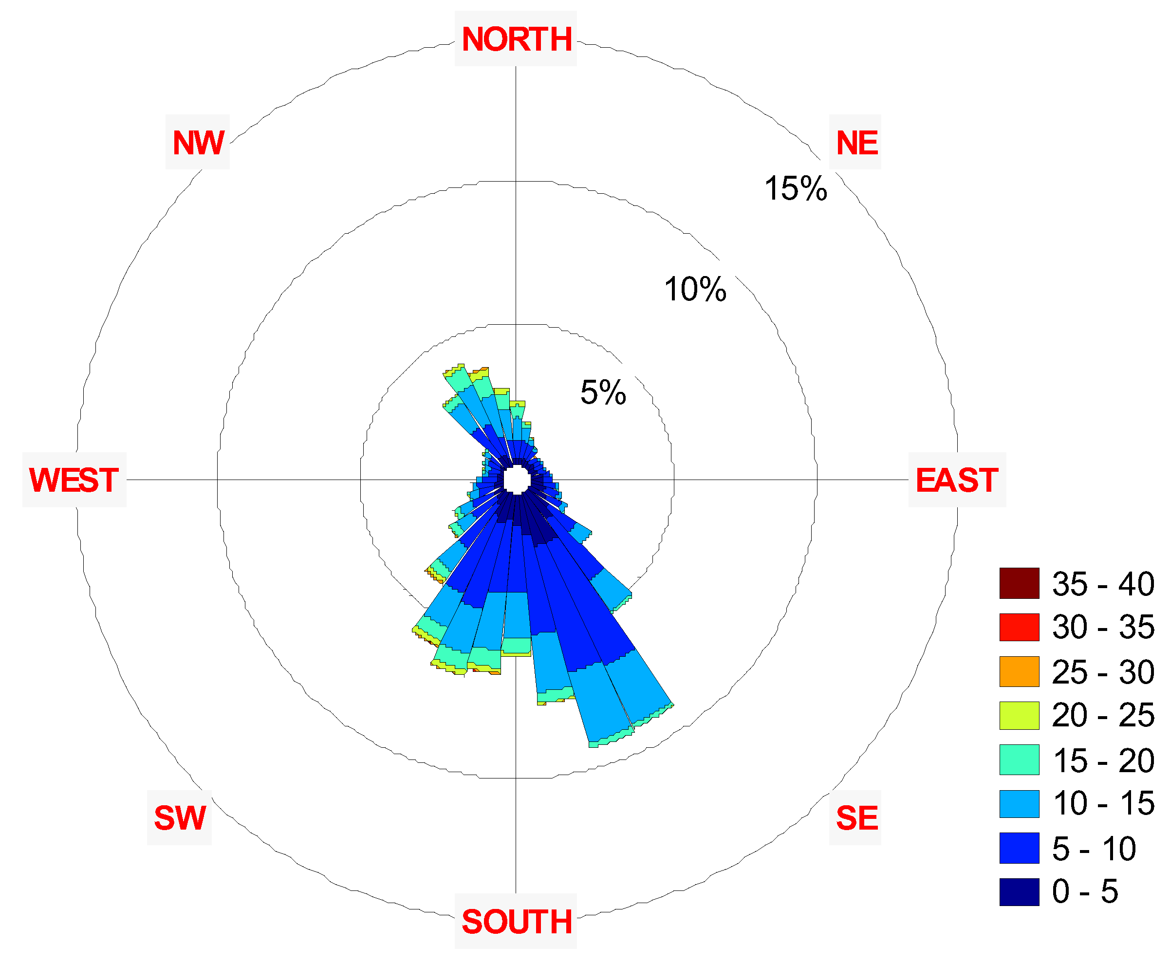
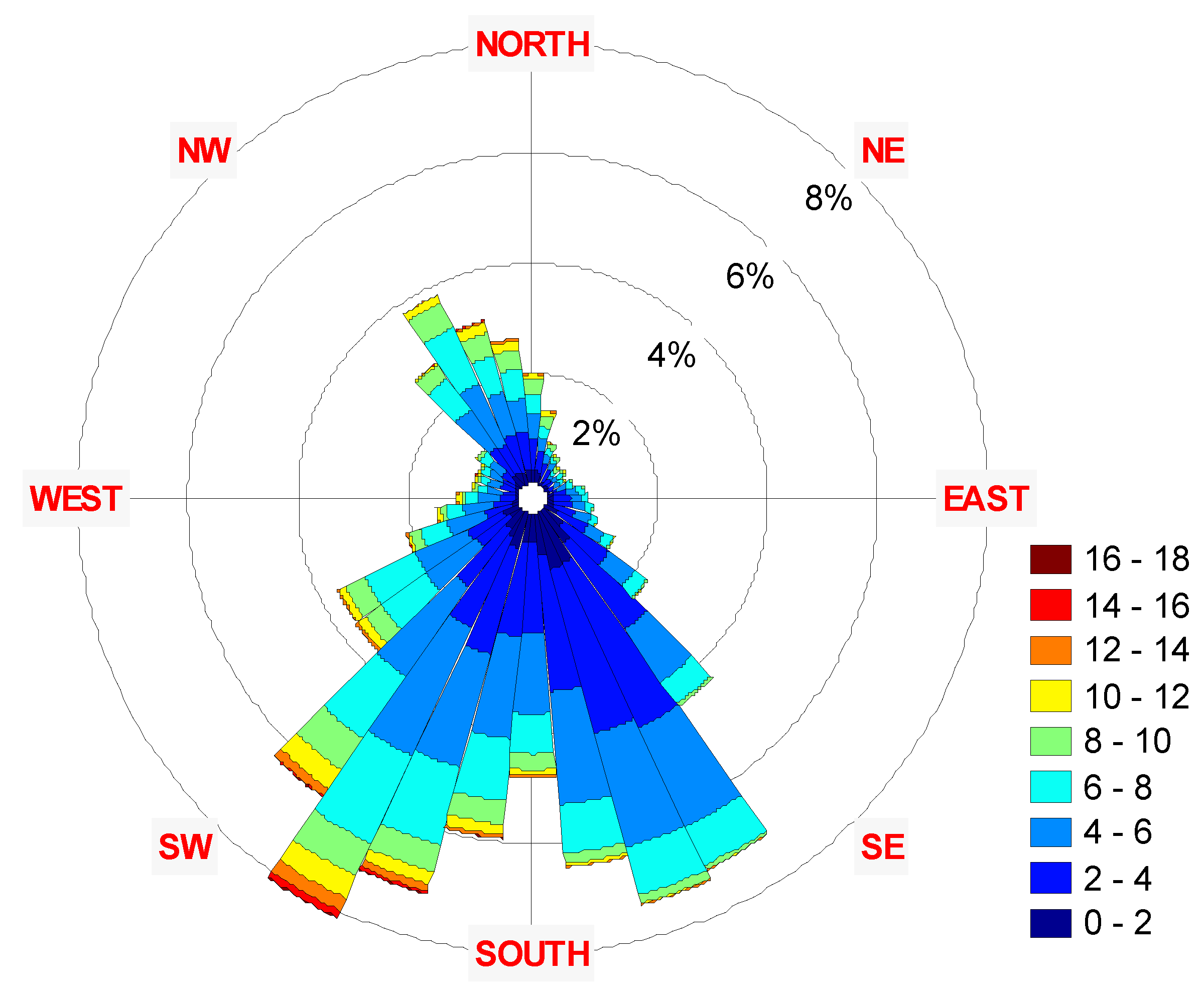
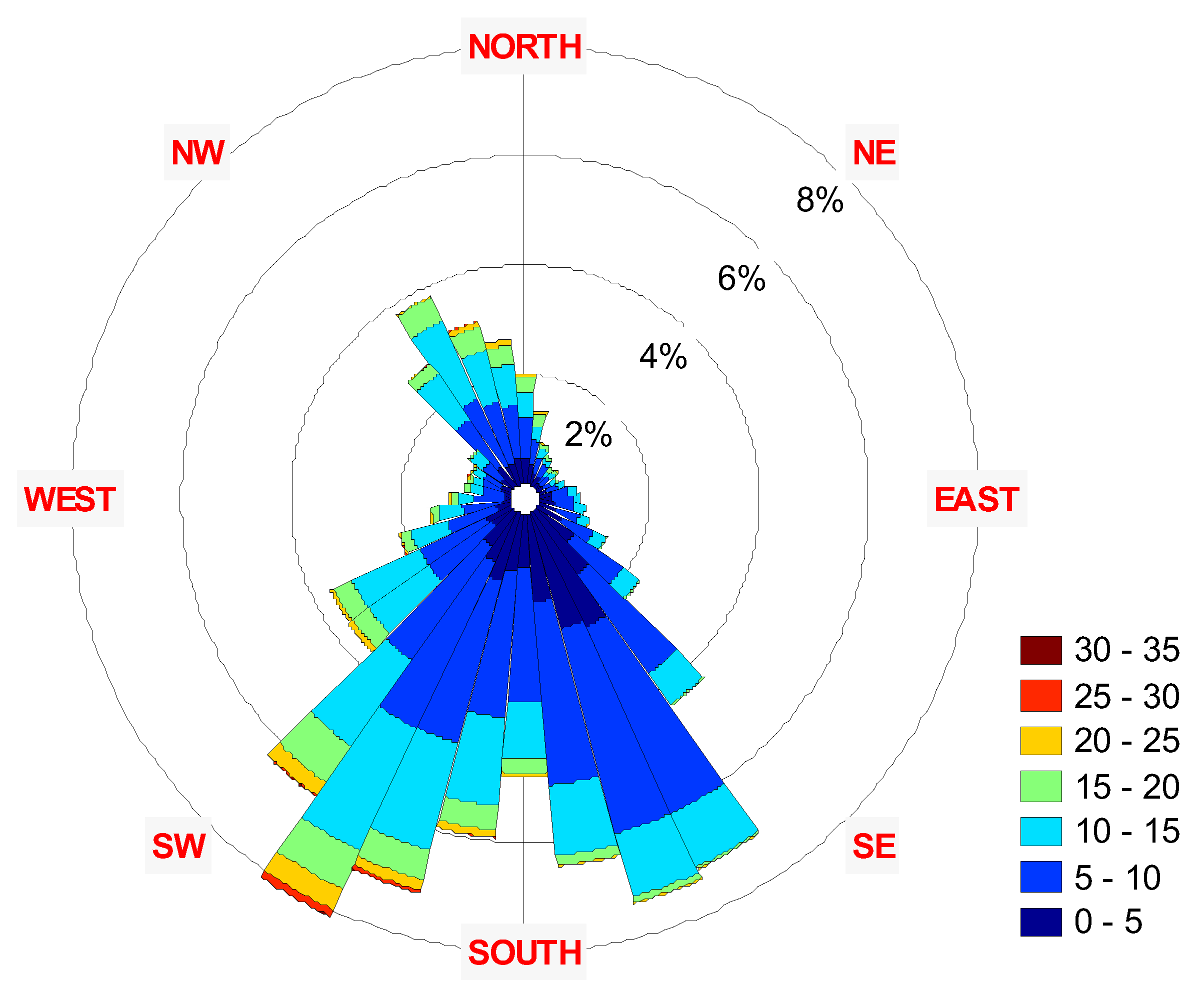
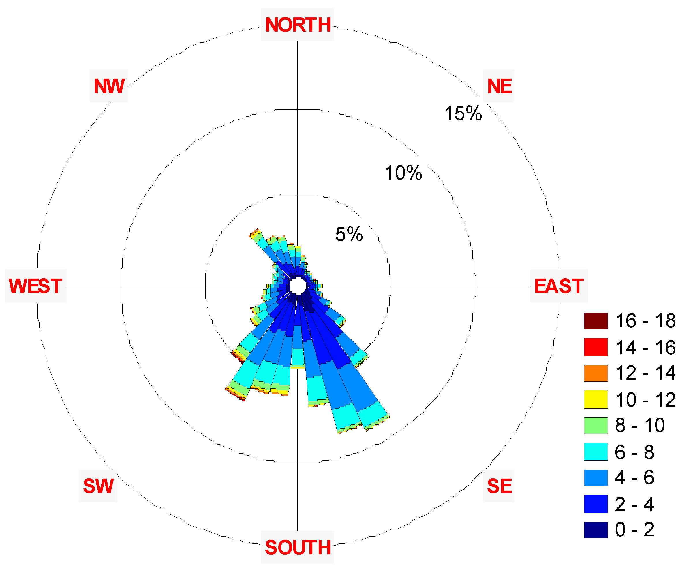
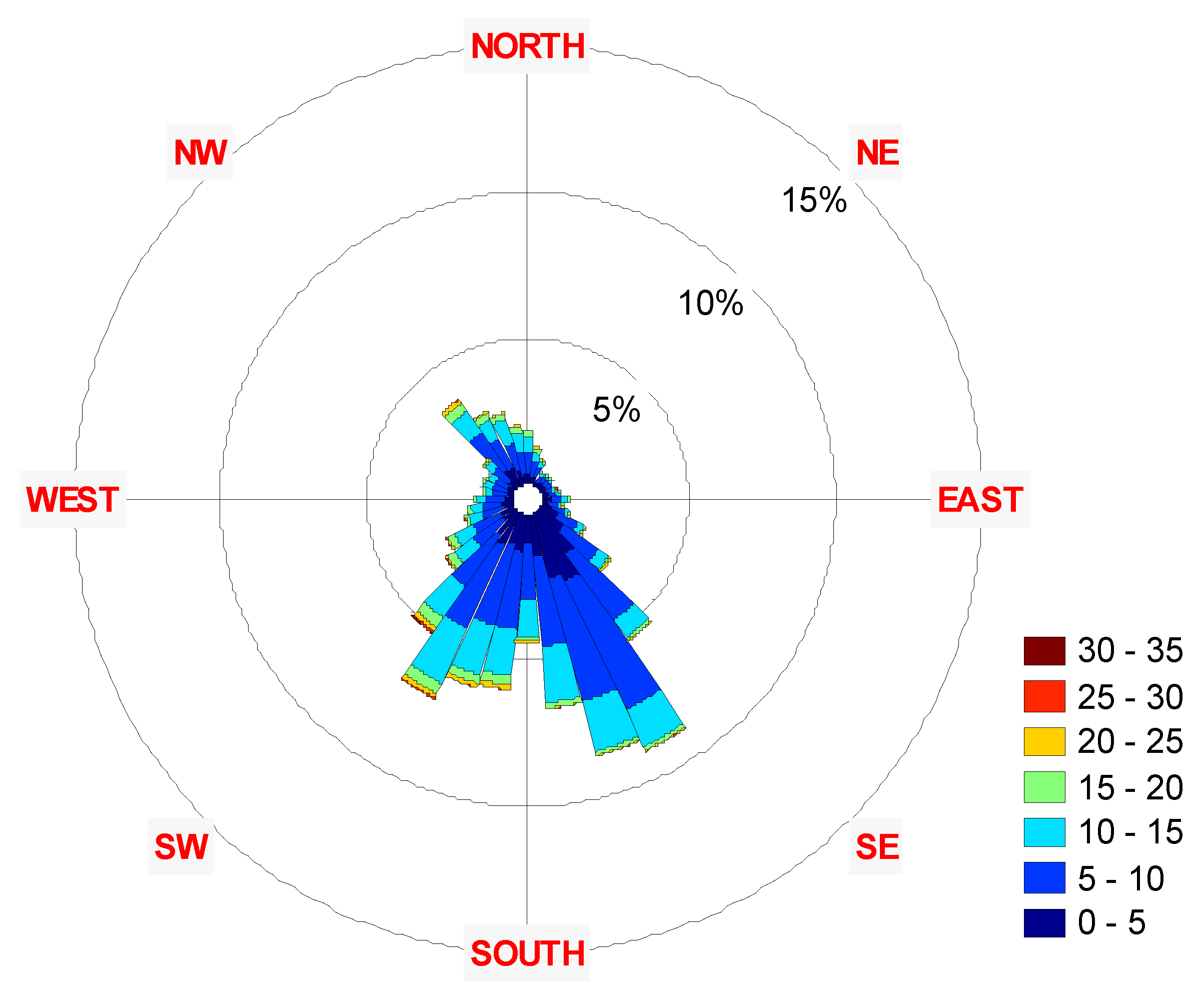

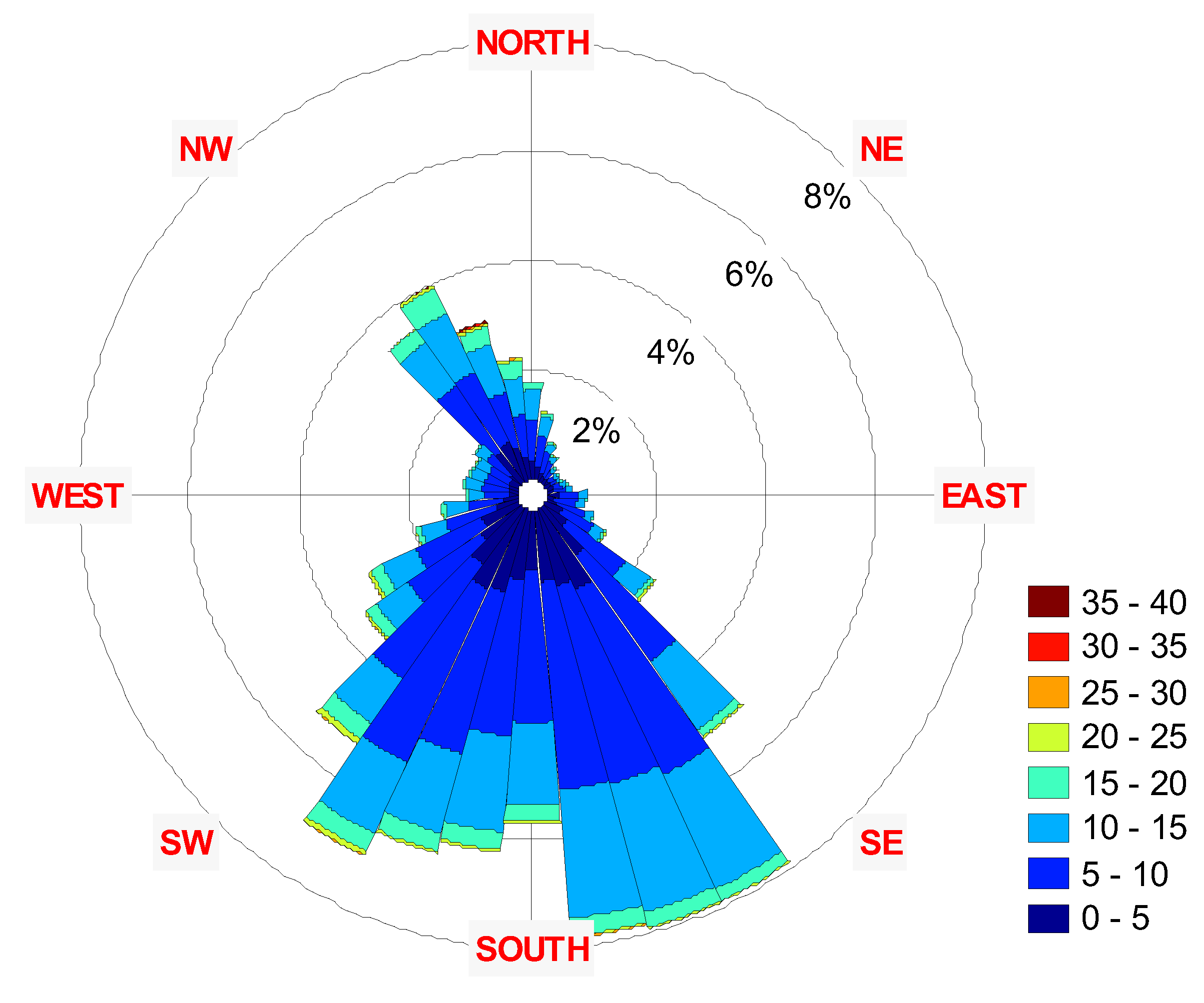
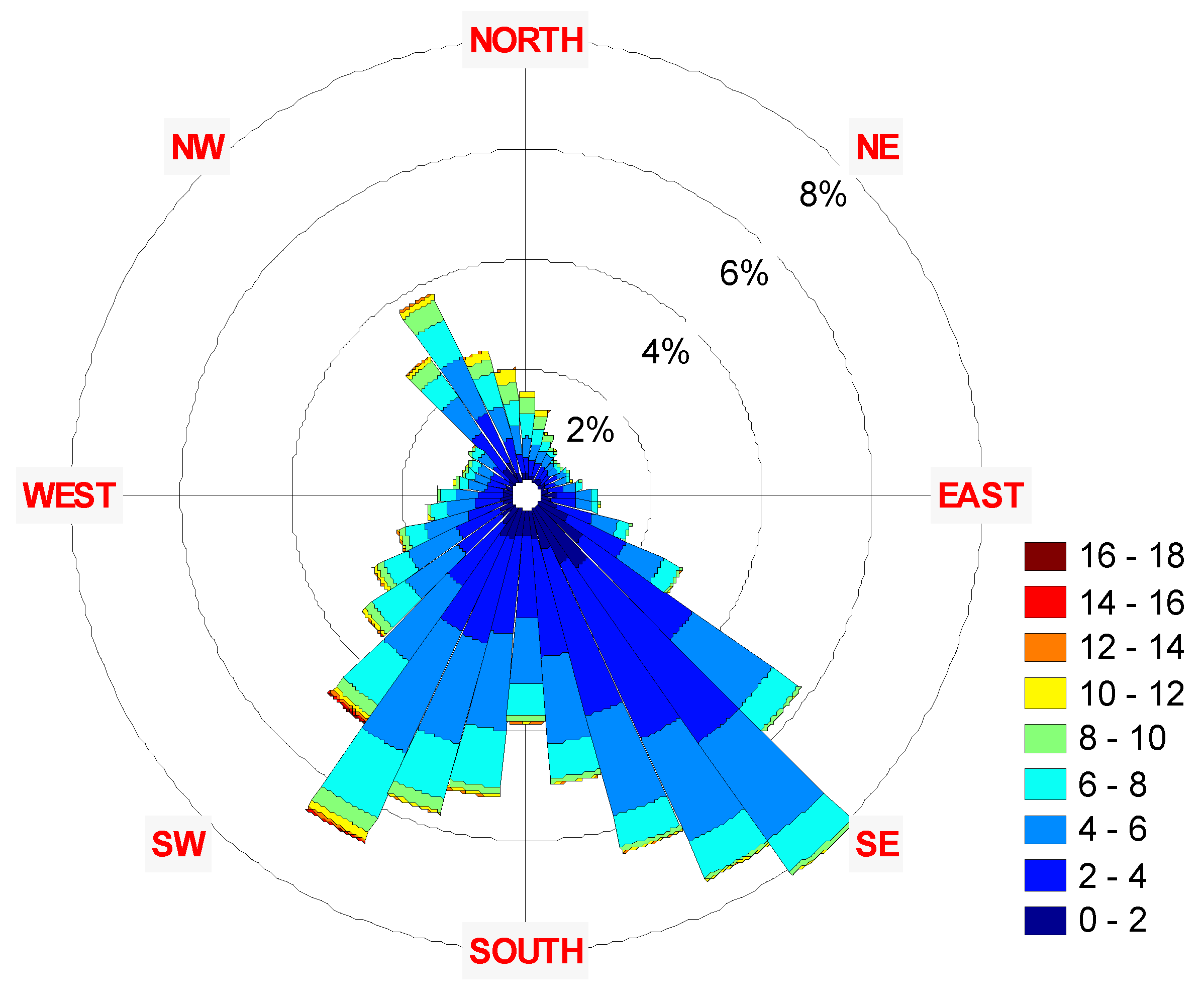
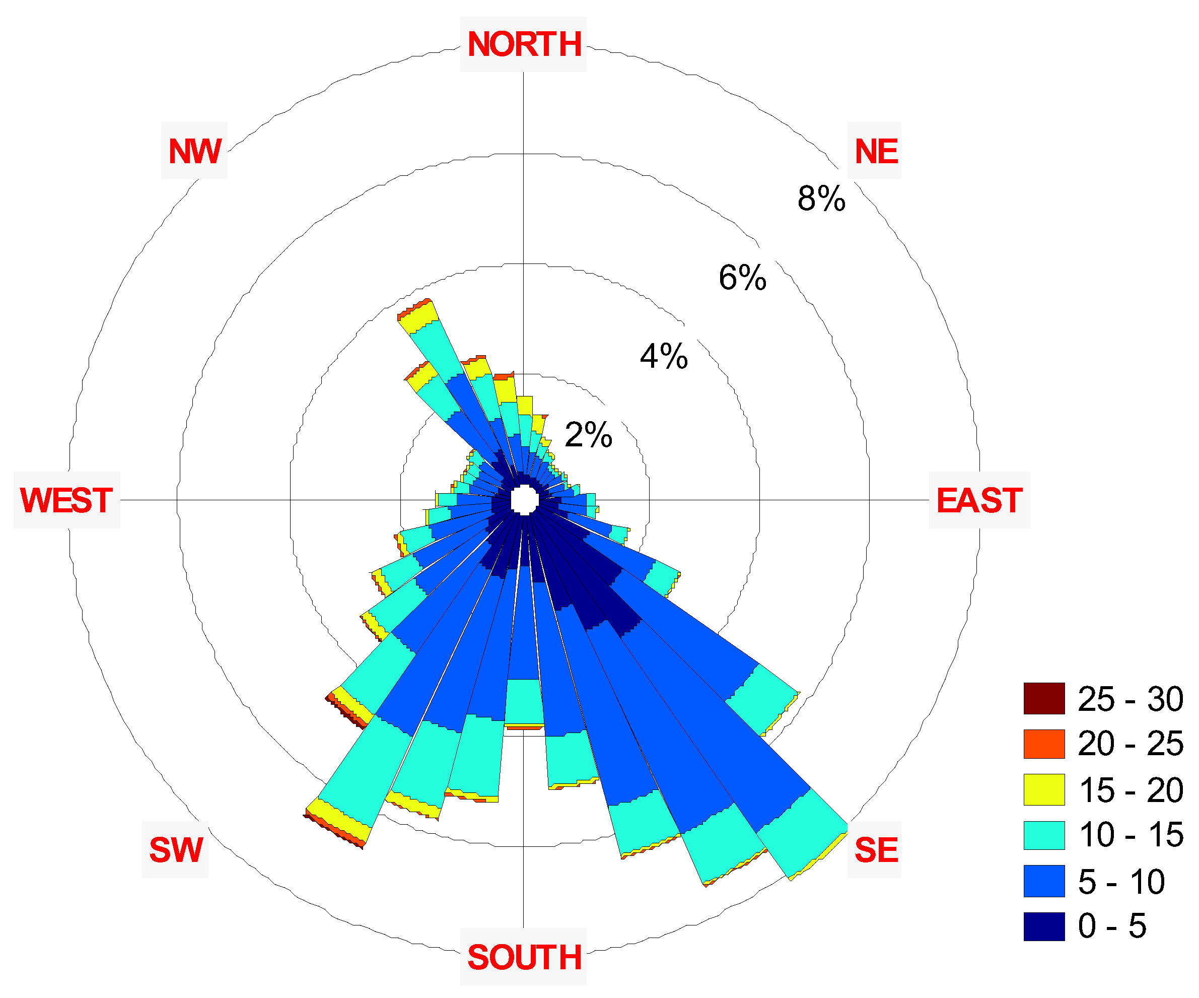
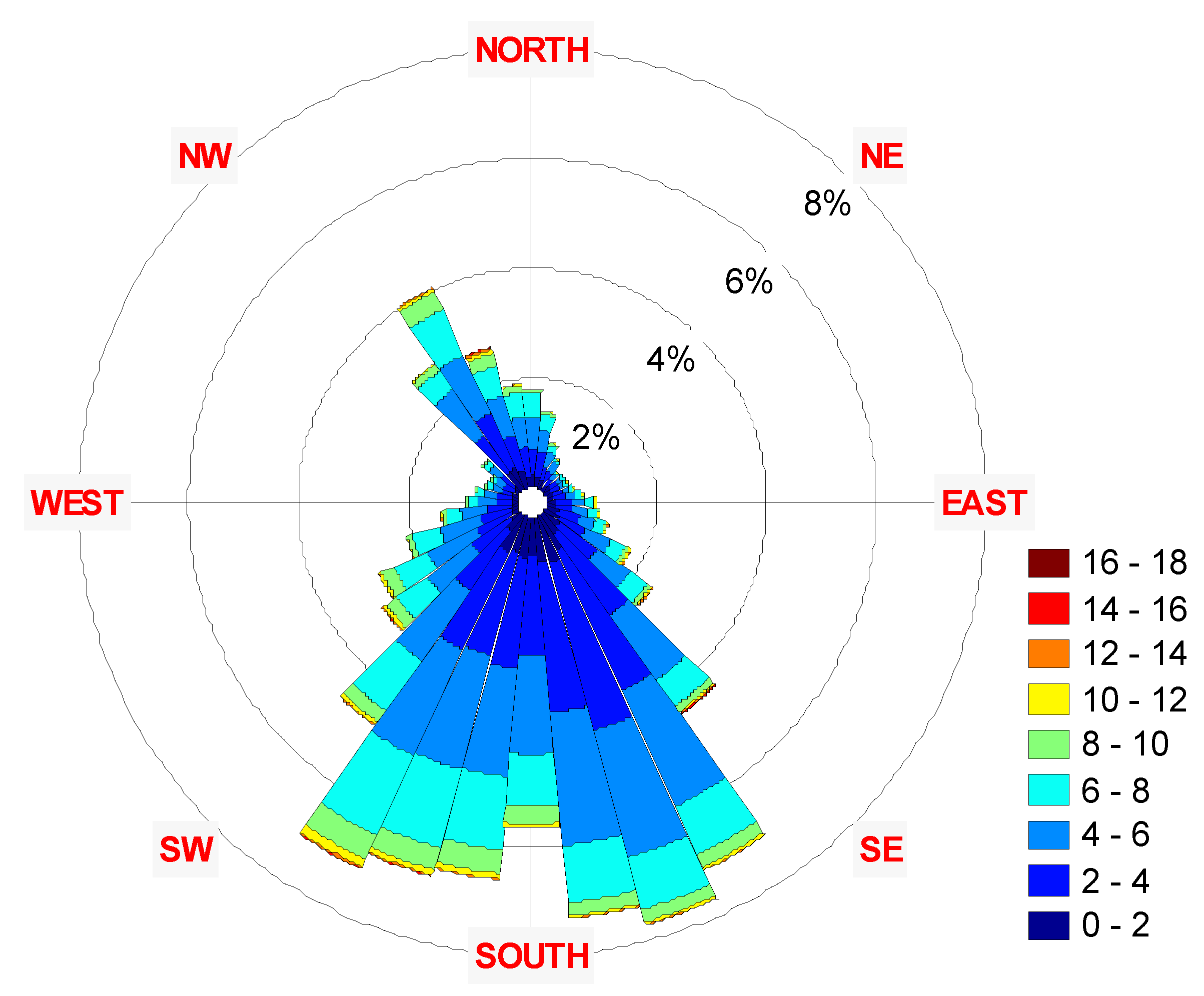
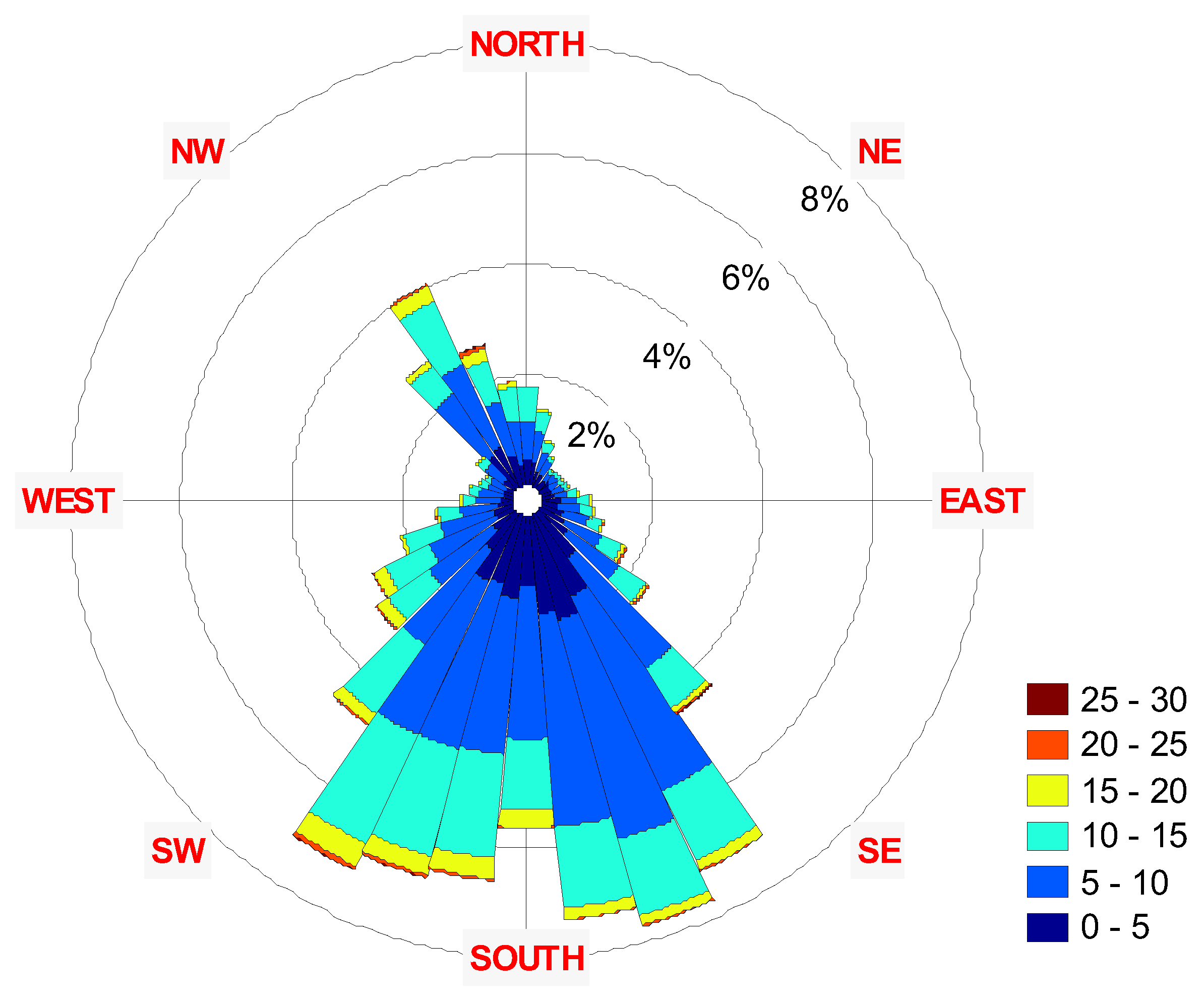
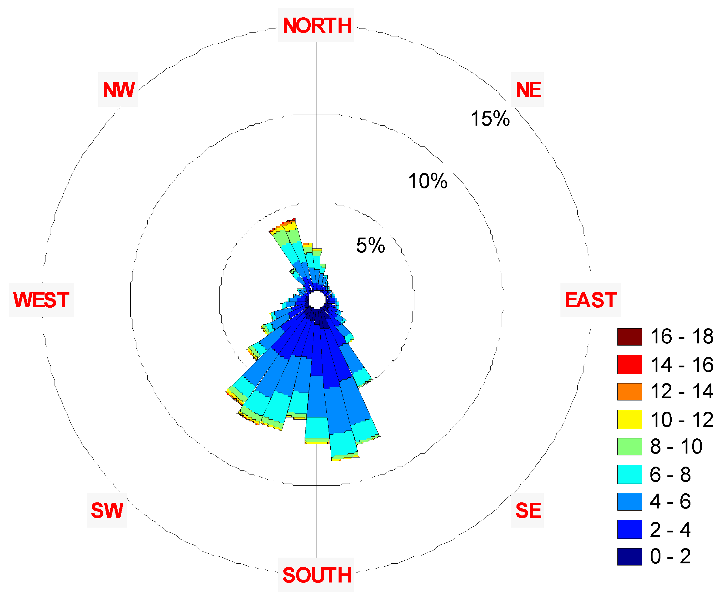


| Wind Power Class |
Average Wind Speed (m/s) at 10 m Height |
|---|---|
| 1 | 0 – 4.4 |
| 2 | 4.4 – 5.1 |
| 3 | 5.1 – 5.6 |
| 4 | 5.6 – 6.0 |
| 5 | 6.0 – 6.4 |
| 6 | 6.4 – 7.0 |
| 7 | 7.0– 9.5 |
| Terrain Characteristics | α |
|---|---|
| Smooth hard ground, calm water | 0.10 |
| Tall grass on level ground | 0.15 |
| High crops, hedges and shrubs | 0.20 |
| Wooded countryside, many trees | 0.25 |
| Small town with trees and shrubs | 0.30 |
| Large city with tall building | 0.40 |
| Year | Parameter | Speed | Azimuth |
|---|---|---|---|
| 2001 | Mean | 4.28 | 209.41 |
| STD | 2.21 | 81.13 | |
| 2002 | Mean | 4.89 | 227.31 |
| STD | 2.51 | 83.03 | |
| 2003 | Mean | 4.81 | 224.15 |
| STD | 2.57 | 78.48 | |
| 2004 | Mean | 4.57 | 228.17 |
| STD | 2.49 | 80.32 | |
| 2005 | Mean | 4.64 | 227.63 |
| STD | 2.33 | 77.45 | |
| 2006 | Mean | 4.35 | 231.65 |
| STD | 2.20 | 83.15 | |
| 2007 | Mean | 4.50 | 228.73 |
| STD | 2.21 | 79.28 | |
| 2008 | Mean | 4.50 | 221.94 |
| STD | 2.25 | 77.23 | |
| 2009 | Mean | 4.54 | 231.31 |
| STD | 2.38 | 75.39 | |
| 2010 | Mean | 4.41 | 225.30 |
| STD | 2.27 | 79.84 | |
| 2011 | Mean | 4.26 | 230.11 |
| STD | 2.08 | 79.28 | |
| 2001-2011 | Mean | 4.53 | 226.00 |
| STD | 2.32 | 79.76 |
| Year | Parameter | Speed | Azimuth |
|---|---|---|---|
| 2001 | Mean: | 7.72 | 209.41 |
| STD: | 3.94 | 81.13 | |
| 2002 | Mean: | 8.78 | 227.31 |
| STD: | 4.50 | 83.03 | |
|
2003 |
Mean: | 8.68 | 224.15 |
| STD: | 4.57 | 78.48 | |
|
2004 |
Mean: | 8.24 | 228.17 |
| STD: | 4.43 | 80.32 | |
|
2005 |
Mean: | 8.37 | 227.63 |
| STD: | 4.15 | 77.45 | |
|
2006 |
Mean: | 7.82 | 231.65 |
| STD: | 3.94 | 83.15 | |
|
2007 |
Mean: | 8.07 | 228.73 |
| STD: | 3.97 | 79.28 | |
|
2008 |
Mean: | 8.07 | 221.94 |
| STD: | 4.04 | 77.23 | |
|
2009 |
Mean: | 8.15 | 231.31 |
| STD: | 4.28 | 75.39 | |
|
2010 |
Mean: | 7.91 | 225.30 |
| STD: | 4.08 | 79.84 | |
| 2011 | Mean: | 7.64 | 230.11 |
| STD: | 3.74 | 79.28 | |
| 2001-2011 | Mean: | 8.13 | 226.00 |
| STD: | 4.17 | 79.76 |
 |
 |
 |
| Parameter | 2001 | 2002 | 2003 | 2004 | 2005 | 2006 | 2007 | 2008 | 2009 | 2010 | 2011 | |
|---|---|---|---|---|---|---|---|---|---|---|---|---|
|
winter Nov-Jan |
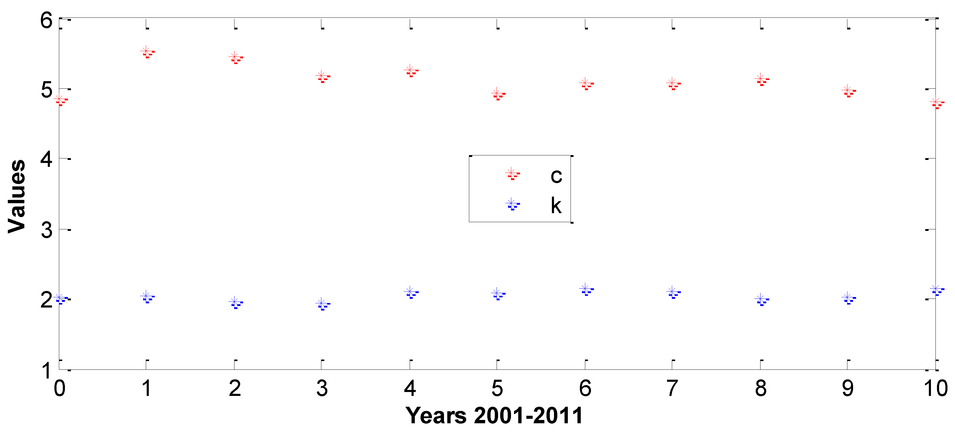
c | 4.53 | 5.25 | 5.48 | 5.03 | 4.67 | 4.99 | 5.08 | 5.86 | 5.51 | 5.68 | 4.94 |
| k | 1.85 | 2.12 | 2.13 | 2.29 | 1.88 | 2.21 | 2.35 | 2.04 | 1.83 | 1.99 | 2.02 | |
|
Spring Feb-Apr |
c | 4.63 | 5.80 | 5.77 | 5.69 | 6.05 | 5.38 | 4.75 | 5.58 | 5.66 | 5.26 | 5.30 |
| k | 1.84 | 2.29 | 2.06 | 2.18 | 2.26 | 1.96 | 2.20 | 2.23 | 1.95 | 1.93 | 1.97 | |
|
Summer May-Jul |
c | 5.33 | 5.58 | 4.80 | 4.84 | 5.37 | 4.65 | 5.94 | 4.55 | 4.87 | 4.83 | 4.72 |
| k | 2.00 | 2.10 | 2.05 | 1.92 | 1.99 | 2.03 | 2.62 | 2.35 | 2.24 | 2.34 | 2.58 | |
|
Autumn Aug-Oct |
c | 4.53 | 5.43 | 5.21 | 4.75 | 5.48 | 5.23 | 4.90 | 4.33 | 4.50 | 4.14 | 4.29 |
| k | 2.39 | 2.08 | 2.08 | 2.05 | 2.05 | 1.99 | 2.51 | 2.30 | 2.41 | 2.36 | 2.50 |
| Parameter | 2001 | 2002 | 2003 | 2004 | 2005 | 2006 | 2007 | 2008 | 2009 | 2010 | 2011 | |
|---|---|---|---|---|---|---|---|---|---|---|---|---|
|
winter Nov-Jan |
c | 8.12 | 9.42 | 9.82 | 9.03 | 8.37 | 8.95 | 9.11 | 10.51 | 9.88 | 10.18 | 8.85 |
| k | 1.85 | 2.12 | 2.13 | 2.29 | 1.88 | 2.21 | 2.35 | 2.04 | 1.83 | 1.99 | 2.02 | |
|
Spring Feb-Apr |
c | 8.31 | 10.41 | 10.34 | 10.21 | 10.84 | 9.64 | 8.52 | 10.01 | 10.14 | 9.44 | 9.50 |
| k | 1.84 | 2.29 | 2.06 | 2.18 | 2.26 | 1.96 | 2.20 | 2.23 | 1.95 | 1.93 | 1.97 | |
|
Summer May-Jul |
c | 9.55 | 10.01 | 8.60 | 8.68 | 9.62 | 8.34 | 10.64 | 8.16 | 8.73 | 8.67 | 8.47 |
| k | 2.00 | 2.10 | 2.05 | 1.92 | 1.99 | 2.03 | 2.62 | 2.35 | 2.24 | 2.34 | 2.58 | |
|
Autumn Aug-Oct |
c | 8.12 | 9.73 | 9.34 | 8.51 | 9.83 | 9.38 | 8.79 | 7.76 | 8.07 | 7.42 | 7.68 |
| k | 2.39 | 2.08 | 2.08 | 2.05 | 2.05 | 1.99 | 2.51 | 2.30 | 2.41 | 2.36 | 2.50 |
| Turbine | Enercon’s E101/3000 | AWE’s 54–900 | EWT’s Directwind 52/750 |
|---|---|---|---|
| Area (m2) | 8012 | 2290 | 2083 |
| Radius (m) | 50.5 | 27 | 25.75 |
| Turbine | Enercon‘s E101/3000 | AWE’s 54–900 | EWT’s Directwind 52/750 |
|---|---|---|---|
| Average Power (kW) | 1380.97 | 379.06 | 333.25 |
| Power Standard Deviation (kW) | 1160.94 | 326.58 | 275.32 |
| Annual Revenue (Million SH) | 6.46 | 1.77 | 1.56 |
| Annual Revenue (Million $) | 1.84 | 0.50 | 0.44 |
Disclaimer/Publisher’s Note: The statements, opinions and data contained in all publications are solely those of the individual author(s) and contributor(s) and not of MDPI and/or the editor(s). MDPI and/or the editor(s) disclaim responsibility for any injury to people or property resulting from any ideas, methods, instructions or products referred to in the content. |
© 2023 by the authors. Licensee MDPI, Basel, Switzerland. This article is an open access article distributed under the terms and conditions of the Creative Commons Attribution (CC BY) license (http://creativecommons.org/licenses/by/4.0/).


