Preprint
Article

Heart Rate Estimation by Video-Based Reflec-tance Photoplethysmography

Altmetrics

Downloads

247

Views

141

Comments

0

This version is not peer-reviewed

Submitted:

23 February 2023

Posted:

24 February 2023

You are already at the latest version

Alerts
Abstract
Non-invasive heart rate (HR) monitoring is important in clinical settings as it plays a critical role in diagnosing a range of health conditions and assessing well-being. Presently, the gold standards for HR measurement are all based on sensors which require skin contact. Apart from inconvenience, contact sensors have proven problematic in certain scenarios – they cannot be used when mechanical isolation of the patient is imperative (burn victims, patients with shaky hands and feet), cause skin damage to premature babies in the ICU and increase the risk of spreading infections. Non-contact HR monitoring using a camera has been recently shown to be a viable alternative. It is now possible to record cardiac-synchronous blood volume variations from facial videos of human subjects under ambient lighting. These variations produce corresponding changes in skin reflectance which can be extracted as a raw reflectance photoplethysmography (rPPG) signal and processed to reveal HR. In this project, an algorithmic framework for webcam-based HR detection was successfully implemented in MATLAB. The investigation was based on 100 self-captured videos (dark-skinned subject) and 48 videos (from 12 subjects, all but one fair-skinned) obtained from COHFACE – an online database of facial videos and corresponding physiological signals. While the performance metrics (mean error, SNR) of the rPPG signals obtained from the self-captured videos were poor (best case mean error of 22%), they were good enough to demonstrate the success of the implementation. The poor results were primarily imputed to skin tone as rPPG SNR is known to be particularly low for dark tones. The results of the COHFACE videos were far superior, with mean error ranging from 3% to 15% (among 8 different rPPG signals) and 0% to 9% under ambient and dedicated lighting, respectively. This investigation sets the foundation for future research directed at optimizing rPPG performance metrics for dark-skinned subjects.
Keywords: 
Subject: Biology and Life Sciences  -   Biology and Biotechnology

1. Introduction

This chapter establishes the aim and rationale of the research reported in this thesis, discusses the relevant theory and associated problems, and enumerates research objectives. It concludes with an outline of the remainder of the thesis.

1.1. Aim of Thesis

The primary aim of this thesis is to implement an algorithmic framework for video-based non-contact heart rate (HR) estimation using the principle of reflectance photoplethysmography (rPPG). It is intended as a foundation for further research devoted to the optimization of rPPG performance metrics for dark-skinned subjects (for which performance is notably poor).

1.2. Rationale for Non-Contact Heart Rate Monitoring

Non-invasive measurement and monitoring of HR is important in clinical settings, as it plays a critical role in diagnosing a range of health conditions and evaluating general well-being. At present, the gold standards for HR measurement are all based on electronic or optical sensors (e.g., ECG and pulse oximeter) which require skin contact (Kumar, Veeraraghavan, and Sabharwal 2015).
Apart from basic inconvenience and discomfort, contact sensors have proven problematic in certain scenarios – they cannot be used when mechanical isolation of the patient is imperative (burn victims, patients with shaky hands and feet), cause skin damage to premature babies in the ICU and increase the risk of spreading infections (Kumar, Veeraraghavan, and Sabharwal 2015). The pulse oximeter, a representative contact sensor (widely used in clinical applications for measuring HR and/or blood oxygen saturation), presents well-known problems. For example, its utility is significantly impaired for long-term monitoring outside the ICU, where motion artefacts lead to repeated false alerts (Tarassenko et al. 2014). The spring-loaded clips in conventional finger oximeters have also been shown to affect the photoplethysmography (PPG) waveform (Teng and Zhang 2004).
Considering these problems, a method for HR monitoring which obviates the need for electrodes or sensors attached to the patient is a long-awaited prospect. Non-contact methods for HR monitoring using a camera have recently emerged as a viable alternative (Verkruysse, Svaasand, and Nelson 2008, Poh, McDuff, and Picard 2010, Sahindrakar, de Haan, and Kirenko 2011). For example, it is now possible to determine the pulsatile blood volume variations associated with the cardiac cycle from facial videos of human subjects captured up to 2 metres away (using only ambient lighting) (Tarassenko et al. 2014). Variations in blood volume produce corresponding variations in the skin reflectance which can be extracted from video as a raw rPPG signal and processed to reveal HR.
Camera-based HR monitoring has numerous applications – from continuous monitoring of patients in the ICU to monitoring in more mundane scenarios like working in front of a computer (Kumar, Veeraraghavan, and Sabharwal 2015). It is also economically viable, with the cost of digital cameras progressively declining as the technology becomes more omnipresent.
HR monitoring via video camera is not without its problems. Present algorithms demand the restrictive condition that a person be effectively at rest facing a camera to ensure accurate measurements (Kumar, Veeraraghavan, and Sabharwal 2015). Accordingly, the technique is highly prone to motion-induced artefacts, particularly when using webcams in ambient light (Bal 2015). However, unlike the motion-based problems in contact monitoring, the use of a camera indicates when the subject is moving and thereby facilitates remedial action (Tarassenko et al. 2014). Another significant drawback is that the technique does not perform well for subjects with dark skin tones and/or under low lighting conditions (Kumar, Veeraraghavan, and Sabharwal 2015).

1.3. Importance of the Heart Rate

The heart is a muscular organ which acts as a pump that circulates oxygen and nutrient-carrying blood around the body and assists in metabolic waste removal. Accordingly, the HR is one of the most important physiological signals of the human body. It is defined as the number of times the heart contracts per unit time and is often expressed in beats per minute (bpm). The normal resting HR for an adult human is 50 – 90 bpm (Spodick 1993), though it is typically lower during sleep and significantly higher during exercise (> 160 bpm) (American Heart Association 2015). Heart rates below and above the normal range are referred to as bradycardia and tachycardia, respectively (Texas Heart Institute).
HR is closely linked to the of viability of the cardiovascular system and the medical status of a person and thus HR measurement has long been used in medicine for non-invasive evaluation of wellness (Mensink and Hoffmeister 1997). An elevated resting HR is correlated with increased risk of cardiovascular (Dyer et al. 1980, Kannel et al. 1987, Thaulow and Erikssen 1991) and all-cause mortality (Hjalmarson et al. 1990, Gillman et al. 1993), as well as cancer mortality (Persky et al. 1981).
Apart from illness, there are many other determinants of HR, both adjustable (e.g., physical activity, smoking, alcohol, stress, posture) and non-adjustable (e.g., age, sex, race) (Valentini and Parati 2009). HR differs significantly for different activities (e.g., sleeping versus exercising) and can change rapidly with postural changes (Borst et al. 1982) and involuntary events such as cardiac arrhythmia and cardiac arrest (National Heart , National Heart). It increases steadily during exercise and gradually returns to the resting value after exercise. It is a well-known indicator of fitness. Generally, the fitter a person, the lower the HR.
The gold standard for measuring HR is electrocardiography (ECG) (Phua et al. 2012), which involves measuring the electrical impulses generated by the heart muscles with electrodes attached to the skin. Other methods include photoplethysmography (used in this thesis), Doppler ultrasonography, use of a piezoelectric transducer, and ballistocardiography (Lindqvist and Lindelow 2016).

1.4. Fundamental Theory of Photoplethysmography
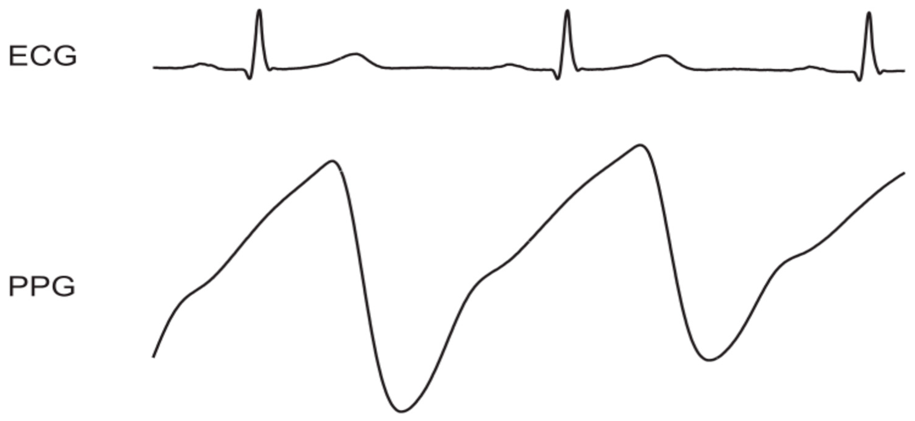
The fundamental theory of photoplethysmography – that pulsatile variations in tissue blood volume modulate the transmission or reflection of visible (or infra-red) light – has been known since the 1930s (Tarassenko et al. 2014). The blood-oxygen transport protein, haemoglobin, is strongly absorptive in visible and near-infrared light. Accordingly, changes in blood volume during the cardiac cycle alter the transmission (or reflection) of light in synchrony with the heartbeat. It is this variation in light transmission or reflection which constitutes the (raw) PPG signal. HR may be extracted from the PPG signal in either the time domain (by measuring the time between consecutive peaks or troughs of the PPG waveform) or the frequency domain (using spectral analysis techniques).
Figure 1.1. AC component of PPG signal compared to ECG. Allen (2007). Reproduced by permission from IOP Science. 
Preprints 69042 g001
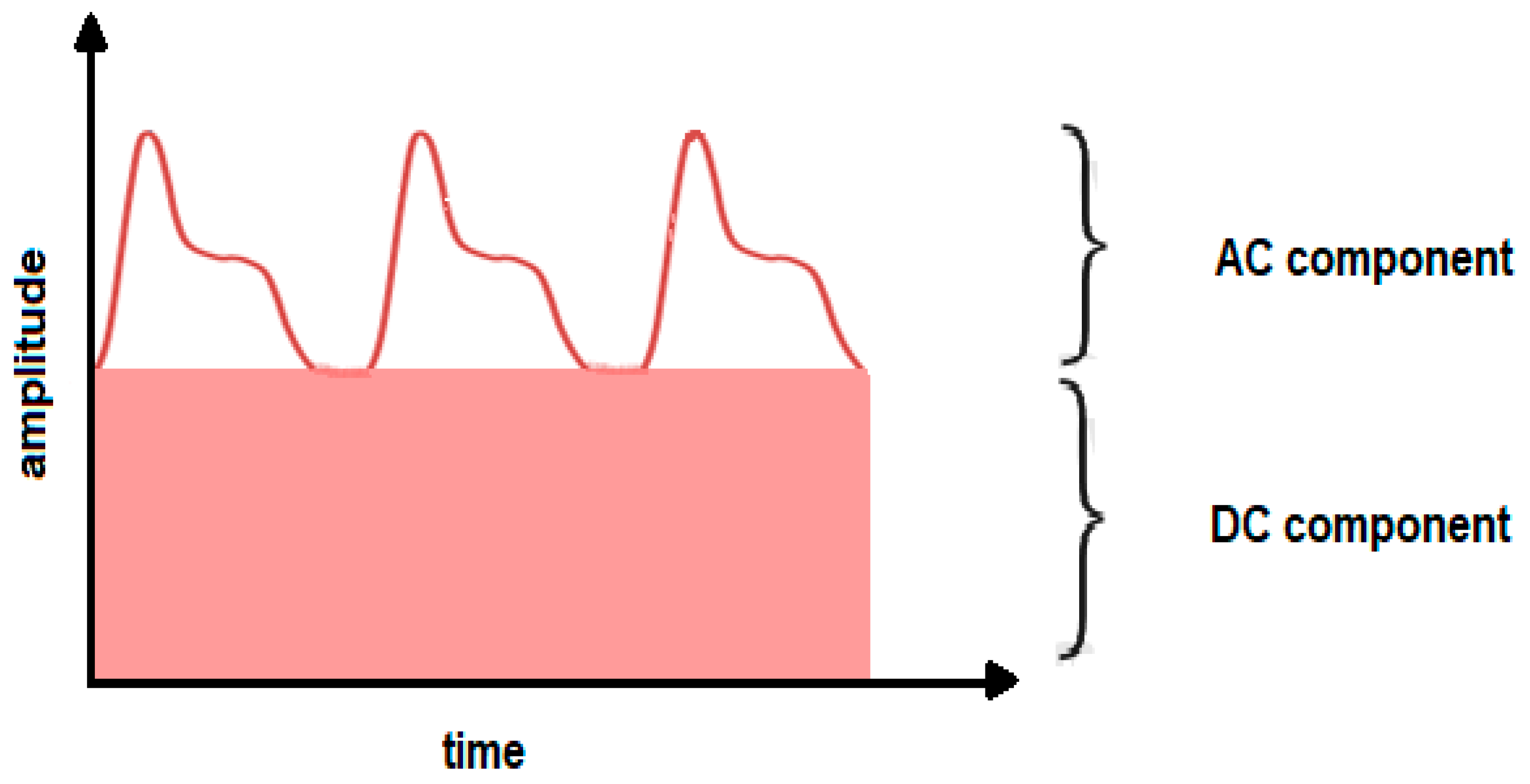
A PPG signal can be obtained from any vascular area of the skin using optical probes in either reflection or transmission mode (Hertzman and Spealman 1937, Nijboer, Dorlas, and Mahieu 1981). After the light is transmitted through or reflected from vascular tissue, it reaches a photodetector and is transduced into current variations which are then amplified and sampled to generate the PPG signal. The PPG signal is made up of two components – a pulsatile AC component and a slowly varying quasi-DC component (Severinghaus 2007, Challoner and Ramsay 1974). The AC component originates from the pulsatile arterial blood (synchronous with HR) while the quasi-DC component is related to non-pulsatile arterial blood, venous blood and other tissues (including bone) (Shao 2016, Saquib et al. 2015). The quasi-DC component also accounts for low frequency events such as respiration, vasometric activity and thermoregulation (Garcia 2013).
Figure 1. 2. AC and DC components of PPG signal.
Preprints 69042 g002
PPG is most commonly associated with pulse oximetry – a technique for estimating the arterial blood oxygen saturation, SaO2.

1.5. Pulse Oximetry—An Example of Contact PPG

Pulse oximetry was developed in the 1970s as a non-invasive means of estimating SaO2 by measuring the pulsatile variations in the intensity of light transmitted through tissue at two different wavelengths (Severinghaus and Honda 1987). Pulse oximeters operate using red and infrared wavelengths and are sensitive to changes in oxygen saturation because of measurable absorption differences between oxygenated and deoxygenated haemoglobin at these wavelengths (Njoum and Kyriacou 2013).
Most pulse oximeters are designed to operate in transmittance mode (Chan, Chan, and Chan 2013), with a probe attached to the finger or earlobe. Reflectance-mode pulse oximeters (with light source and detector on the same side) are less common and operate by detecting light that has back-scattered from the tissue. They are mainly used in forehead pulse oximetry (Agashe, Coakley, and Mannheimer 2006) for clinical applications involving peripheral shut-down, where transmittance-mode pulse oximeters malfunction due to reduced blood flow in the extremities (Tarassenko et al. 2014).
Figure 1. 3. Transmission (left) and reflection (right) mode contact pulse oximetry. Tamura et al. (2014).
Preprints 69042 g003

1.6. Non-Contact Photoplethysmography
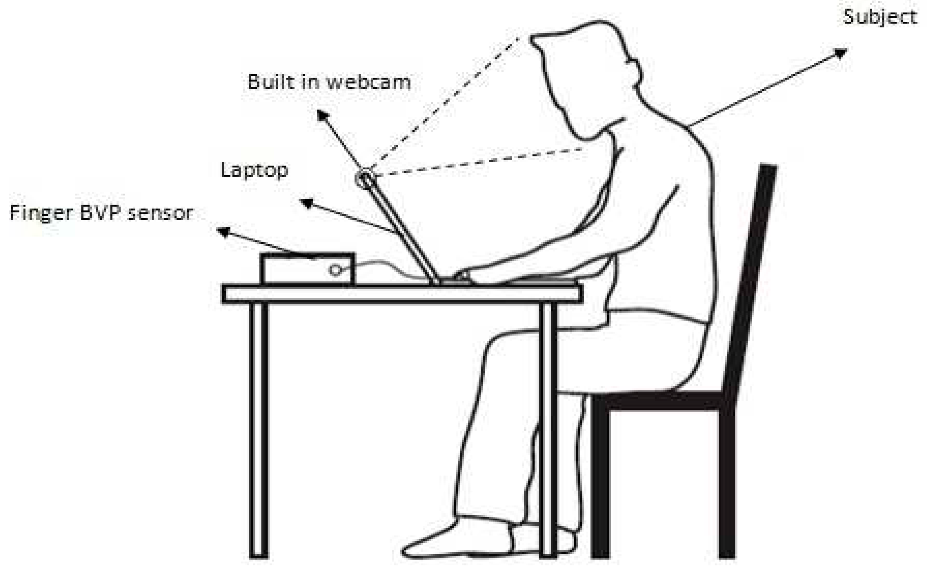
In non-contact PPG, there is no mechanical coupling between sensor and subject. Non-contact PPG, like pulse oximetry, may operate in transmission or reflection mode. This thesis implements video-based non-contact reflectance photoplethysmography, with the camera operating as the sensor of reflected light. Figure 1.4 shows a representative setup for HR estimation by video-based rPPG.
Figure 1. 4. Representative setup for video-based rPPG. Poh et al. (2010).
Preprints 69042 g004

1.7. Problems with Video-Based rPPG

The performance and applicability of video-based rPPG is challenged by three main problems:
  • Intrinsically low signal strength
  • Motion artefacts
  • Noise due to fluctuations in illumination.
The low signal strength arises from the fact that the blood volume perfusing the skin is very small (only 2 – 5% of body total), with an even smaller volume (5% of skin volume) in sync with the HR (Kumar, Veeraraghavan, and Sabharwal 2015). Accordingly, the variations in subsurface skin reflectance due to the cardiac-synchronous fraction of blood volume is also very small. The result is changes in camera-recorded light intensity that are minute relative to changes in surface reflection caused by ordinary motion. Under life-like conditions, this represents patently low signal-to-noise ratio (SNR), which is further degraded for dark skin tones (poor reflectance due to increased melanin) and/or low lighting conditions (Kumar, Veeraraghavan, and Sabharwal 2015).
The motion artefacts and noise contamination are closely related to low signal strength. As discussed, small movements of a subject can lead to large variations in surface reflection which introduce high levels of noise into the weak rPPG signal. Background variations in illumination result in similar contamination. Thus, while relatively noiseless data (with artificially high accuracy) may be obtained under controlled settings, the established techniques significantly underperform in more realistic situations such as monitoring of patients on dialysis (Tarassenko et al. 2014). In such life-like settings, there may be sudden and significant variations in the intensity of ambient light, as well as rigid motions of the head and other less subtle motions (such as changes in facial expression) which significantly compromise the utility of rPPG.
Many investigations have attempted to counter the effects of motion. Poh et al., for example, attempted to reduce motion artefacts by using automatic face detection to track the face from frame to frame (2010). They, however, limited the motion to slow and uniform head swings. Still, the technique was fraught with difficulties in continuously detecting moving faces, with the researchers reporting a large number of false-negatives.
A comparable method computes 2D shifts in the location of the face between frames and uses image correlation to model the motion (Yu et al. 2011). This method also has its limitations as it can only capture the basic translational motion of the face and is unable to effectively compensate for more life-like motion such as the turning or tilting of the face, or the change in the contours of the face that come with smiling or talking.

1.8. Research Objectives

The primary research objectives of this thesis are to:
  • Implement an algorithmic framework for HR estimation by video-based reflectance photoplethysmography
  • Investigate the effect of the presence/absence of dedicated lighting on the SNR of rPPG signals
  • Investigate the effect of choice/size of the region of interest (ROI) on the SNR of rPPG signals
  • Compare the SNR of green rPPG signals with that of rPPG signals based on luminance
  • Investigate the viability of the use of the summary autocorrelation function (SACF) as a technique for improving the SNR of rPPG signals
  • Implement the HR estimation algorithm into a graphical user interface (GUI)
  • Prepare a laboratory practical centred on HR estimation by video-based rPPG

1.9. Thesis Outline

This thesis is organised as follows:
Chapter 2 presents a literature review of previous work on various implementations of HR estimation by reflectance photoplethysmography and its precursors. Chapter 3 itemizes the materials used for carrying out this investigation and discusses the experimental setups. Chapter 4 continues the discussion on materials and methods in terms of the implementation workflow and algorithms. Chapter 5 presents the results of the study, while Chapter 6 discusses the results. Chapter 7 summarises the findings, draws conclusions and makes recommendations for future work.

2. Literature Review

This chapter reviews the literature relevant to an implementation of video-based rPPG.

2.1. Previous Work

The first non-contact HR estimation system was designed by Da Costa using two optical methods to record the cardiac-synchronous deflection of a human vein (1995). In the first method, the skin in the region of the vein is illuminated using a 2 mW HeNe laser and the reflected speckle pattern is recorded with a TV camera. The speckle contrast is then computed across frames and represented as a time series (from which HR can be determined). In the second method, the position of a light spot formed by laser light reflected from a small mirror glued to the skin is recorded by a CCD camera and plotted as a function of time. Since the displacement of the mirror is synchronized with that of the vein, HR can be extracted from the fluctuations of the spot position. The investigation, however, failed to report quantitative results or any correlation with reference ECG measurements (Kumar, Veeraraghavan, and Sabharwal 2015).
Following Da Costa’s initial attempt, further progress was moderate until Wieringa et al. showed, for the first time, that it is possible to derive rPPG signals from backscattered light detected by a monochrome CMOS camera (2005). The signals were acquired from the left inner arm (near the wrist) of seven volunteers (positioned 0.7 m away from the camera) by sequential illumination with non-coherent light at three different wavelengths. All signals contained a pulsatile component correlated with breathing and a smaller amplitude component at the cardiac frequency.
In a similar investigation, Humphreys et al., using a CMOS camera, obtained rPPG signals from light reflected off the inner arm of ten volunteers (2007). An array of LEDs (at two different wavelengths – 760 and 880 nm) served as the light source, allowing two multiplexed rPPG signals to be obtained concurrently at a rate of 16 frames per second (fps). HR estimates from the rPPG signals showed excellent agreement with reference pulse oximeter values.
Takano et al. also showed that it is possible to simultaneously extract HR and BR using a CCD camera (2007). They recorded images of a selected region of a subject’s skin and then determined the variations in the average intensity of the ROI over a period of 30 s. The intensity data was then processed using standard MATLAB functions for filtering and spectral analysis. Both HR and BR showed very high correlation with reference values.
Another noteworthy study reported a non-contact method for determining HR based on the analysis of thermal images (Garbey et al. 2007). The study revealed that the temperature of blood vessels is modulated by pulsatile blood flow, resulting in a thermal signal from which HR can be extracted after appropriate processing. The thermal signal also yields quantitative information about respiratory function and blood flow velocity.
Perhaps the most important recent development in camera-based rPPG is the ability to monitor vital signs using facial videos under ambient light (Verkruysse, Svaasand, and Nelson 2008, Poh, McDuff, and Picard 2010, 2011, Kwon, Kim, and Park 2012, Balakrishnan, Durand, and Guttag 2013). Verkruysse et al. showed, for the first time, that rPPG signals could be acquired from face videos in ambient illumination using a consumer grade digital camera positioned greater than 1 metre (2008). The video analysis involved the selection of ROIs in each frame of the face (usually the forehead) and the calculation of the mean pixel intensity of the ROIs to form the raw rPPG signal. The raw signal was bandpass filtered using a fourth-order Butterworth filter with cut-off frequencies of 0.8 – 6 Hz (corresponding to heart rates of 48 and 360 bpm). The filtered signals were then subjected to FFT over a 10 s window and the HR was determined from the frequency content.
The Verkruysse study found the face (particularly the forehead) to be the best surface for extracting rPPG signals because of improved SNR. The study also demonstrated that the green channel of an RGB camera outperforms the red and blue channels for detecting HR and BR. This is not surprising since it is known that the absorption spectra of haemoglobin and oxyhaemoglobin – the primary color agents in blood – have absorption peaks in the passband range of the green filters in color cameras (Kumar, Veeraraghavan, and Sabharwal 2015). A supplementary discovery is that cyan, orange and green (COG) channels work better than RGB (McDuff, Gontarek, and Picard 2014).
The work of Poh et al. (2010) represents a notable attempt to improve on the foundation laid by Verkruysse et al., particularly with respect to motion robustness. Using the webcam of a Macbook Pro, positioned about 0.5 m from the subject, the researchers simultaneously detected the HR, HRV and BR of 12 volunteers with varying complexion. The studies were conducted indoors at day-time, with varying intensities of ambient illumination. The improvement in motion robustness was achieved using continuous automatic face detection based on the Viola-Jones and Lienhart-Maydt face detectors (Viola and Jones 2001, Lienhart and Maydt 2002), and the JADE algorithm for independent component analysis (ICA) (Cardoso 1999) (subsequent investigations have reduced the computational cost of continuous face detection by performing initial face detection followed by the Kanade-Lucas-Tomasi (KLT) algorithm (Lucas and Kanade 1981) for motion tracking (Tarassenko et al. 2014, Li et al. 2014, Kumar, Veeraraghavan, and Sabharwal 2015, Rahman et al. 2016)). Following face detection, the average intensity of the ROI was computed across frames for each RGB channel. The RGB traces were then subjected to ICA to yield three independent signals. The rPPG signal was extracted from one of these independent signals and then Fourier-transformed to determine the peak of maximum amplitude within the range of 0.7 – 4 Hz. This was taken as the HR frequency. The results showed that ICA-decomposed signals can achieve higher accuracy for estimating HR compared to the green signal.
A later study, however, yielded results which contradicted that of Poh et al. with respect to the superiority of ICA separation (Kwon, Kim, and Park 2012). Comparing HR estimates extracted from green signals versus ICA separated signals (from face videos captured by a smartphone camera), the researchers found that ICA slightly underperformed. Poh et al. later designed an improved technique which achieved very accurate HR estimation. It involved the application of several temporal filters before and after ICA (2011).
Sahindrakar et al. (2011) proposed and assessed several improvements on various aspects of framework established by Poh et al. (2010, 2011) (ROI selection, tracking, signal pre-processing etc.), with an overall view to reduce motion artefacts. Though they succeeded in improving SNR, motion artefacts still remain an issue. Particularly interesting among the improvements was the demonstration that the three channels of the RGB space may be combined in various ways to yield rPPG traces of superior SNR compared to the green signal.
In terms of understanding the nature of the rPPG signal, the work of Balakrishnan et al. requires special mention (2013). According to their research, facial rPPG signals are due not only to volume changes in facial blood vessels (Poh, McDuff, and Picard 2010) or color changes in these vessels (Wu et al. 2012), but also involves a third component – ballistocardiographic changes. These are motion-induced changes hypothesized to originate from cyclical movement of blood from heart to head, giving rise to oscillatory motion of the head at the cardiac frequency.
Other noteworthy experiments using digital cameras for vital signs estimation include Yu et al. (2011), Lewandowska et al. (2011), Holton et al. (2013), and Shao et al. (2016).
A chief limitation of the systems discussed thus far is that they are not designed for real-time implementation and are consequently of limited utility in applications such as personal health care and telemedicine. Within the last five years, research has continued to improve techniques, with an increasing focus on making camera-based vital signs monitoring more suitable for real-time applications (Datcu et al. 2013, Zhao et al. 2013, Rahman et al. 2016).
A real-time application of considerable value is the vital signs monitoring of drivers (Rahman, Barua, and Begum 2015, Rahman, Begum, and Ahmed 2015). One implementation used an iSight webcam to capture facial images, separated the image data into three the RGB channels and performed further processing for HR and BR estimation (Zhang et al. 2014). A similar system was developed for continuous monitoring of the HRV of drivers under real-world driving conditions (Guo, Wang, and Shen 2014).
Another significant trend in camera-based vital signs monitoring is a turn towards integration with smartphone technologies (Papon et al. 2015). Apart from monitoring based on the finger in contact with the phone camera (Pelegris et al. 2010, Peng et al. 2015), smartphone systems have also been developed for remote monitoring via facial videos (Kwon, Kim, and Park 2012, Jiang et al. 2014).
The camera-based vital signs monitoring studies discussed thus far originate primarily from the United States. Paralleling work in the US is work by Phillips Research Laboratories in Europe. They have developed similar FFT-based methods for estimating HR from remotely derived PPG signals and BR from motion analysis. This culminated in the release of a software application for the iOS operating system in 2011 (Tarassenko et al. 2014).
There is also significant work at Philips devoted to minimizing the effect of motion artefacts – for example, by using multi-spectral illumination and adaptive filtering techniques (Cennini et al. 2010). There is also focus on issues of motion estimation and compensation (Schmitz 2011, Sahindrakar, de Haan, and Kirenko 2011), with a recent paper dealing with problems related to periodic motion during exercise (Haan and Jeanne 2013).

3. Materials and Methods 1: Experimental Setup

This chapter describes the materials and methods used in this thesis. It begins with an itemized description of materials, followed by a discussion of experimental setup. It also describes the various ROIs used for rPPG signal extraction and sets up a classification for these signals based on choice of ROI, color space component and spectral analysis technique (FFT or Welch periodogram). It concludes with definitions of the performance metrics of the rPPG signals – namely mean error, root-mean-square-error (RMSE) and mean SNR.

3.1. Research Materials

Dell Inspiron 14-3425 PC: for video capture via 0.9-megapixel built-in webcam
HP Pavilion 15 Notebook PC: for signal processing
MATLAB R2017: for coding signal processing algorithms and GUI
COHFACE dataset: an online dataset of 160 facial videos (from 40 healthy subjects under natural and studio lighting) and corresponding physiological signals (contact PPG and respiratory)
Pulse oximeter module: for ground truth HR measurements for lab exercise (research objective 6)
Arduino microcontroller: for interfacing pulse oximeter with computer
MATLAB support package for Arduino: for obtaining ground truth signal in MATLAB environment
Photo Studio LED light: 600 lumens dedicated lighting for self-captured videos

3.2. Experimental Setup

This investigation involved two experimental setups:
self-captured videos (of dark-skinned subject) and
COHFACE database videos

3.2.1. Setup 1—Self-Captured Videos

Fifty (50) videos (each) were shot under ambient and dedicated lighting, respectively. Ambient lighting was composed of a mixture of natural and fluorescent lighting, while dedicated lighting constituted ambient lighting plus an LED light focused on the subject’s face. All videos were shot in the same room to minimize variability in system performance introduced by external factors. The timing of video capture was also chosen to keep ambient light intensity approximately constant.
For every trial, the subject was seated 0.4 – 0.5 m from the camera. The subject was instructed to remain still while facing the camera, with left arm on an arm rest and hand fixed (in order to obtain reliable ground truth information). The distance between the subject and dedicated light source (600 lumens) was approximately 1 metre. Ground truth HR was obtained manually by a medical doctor (counting radial pulse). However, for the laboratory exercise (see research objective 6), the ground truth signal can be obtained from a pulse oximeter module interfaced with a computer (via an Arduino microcontroller). In this case, HR is determined by taking the FFT of the ground truth signal over the length of measurement.
Video capture was achieved using a 0.9-megapixel webcam (built into a Dell Inspiron 14-3452 PC) at 29 fps in most cases (30 fps in all other cases), with a resolution of 720 x 1280. All videos were automatically stored in the MP4 format without any compression, resulting in 24-bit RGB video. However, 12 videos failed facial detection and it was found that conversion to AVI format resolved the problem. Accordingly, these videos were processed for signal extraction in AVI format.

3.2.2. Setup 2—COHFACE Videos

Forty-eight (48) videos from 12 subjects (2 under natural lighting, 2 under studio lighting per subject) were taken from COHFACE – an online dataset of 160 facial videos and corresponding physiological signals from 40 healthy subjects (Heusch, Anjos, and Marcel 2017). The sampling of the 12 subjects involved simply selecting the first 6 males and 6 females in the dataset. The sample was composed of 10 (fair-skinned) Caucasians and 2 (dark-skinned) Indians.
Two illumination conditions were used:
  • Natural (which approximates ambient for self-captured videos): for which all lights were turned off and the blinds were opened, and
  • Studio (which approximates dedicated for self-captured videos): for which the blinds were closed to minimize natural light and extra light from a spot was used to illuminate the subject’s face.1
Each subject was asked to sit still while facing a webcam for four sessions, each lasting approximately 60 s. Physiological signals (contact PPG and respiratory) were taken by a BVP sensor and respiration belt from Thought Technologies at 256 Hz and 32 Hz (respectively) and stored in HDF5 format (which is accessible by built-in MATLAB functions). Both sensors were connected to a computer running Microsoft Windows via 2-channel USB-based acquisition. Data from the sensors, together with the video stream, were synchronized and recorded using Thought Technologies’ BioGraph Infiniti Software suite, version 5.
Videos were captured using a PC with built-in Logitech HD Webcam C525 at 20 fps, with a resolution of 640 x 480 pixels. All videos were stored in AVI format without any compression, resulting in 24-bit RGB video.

3.3. ROI Description and Classification for Associated rPPG Signals
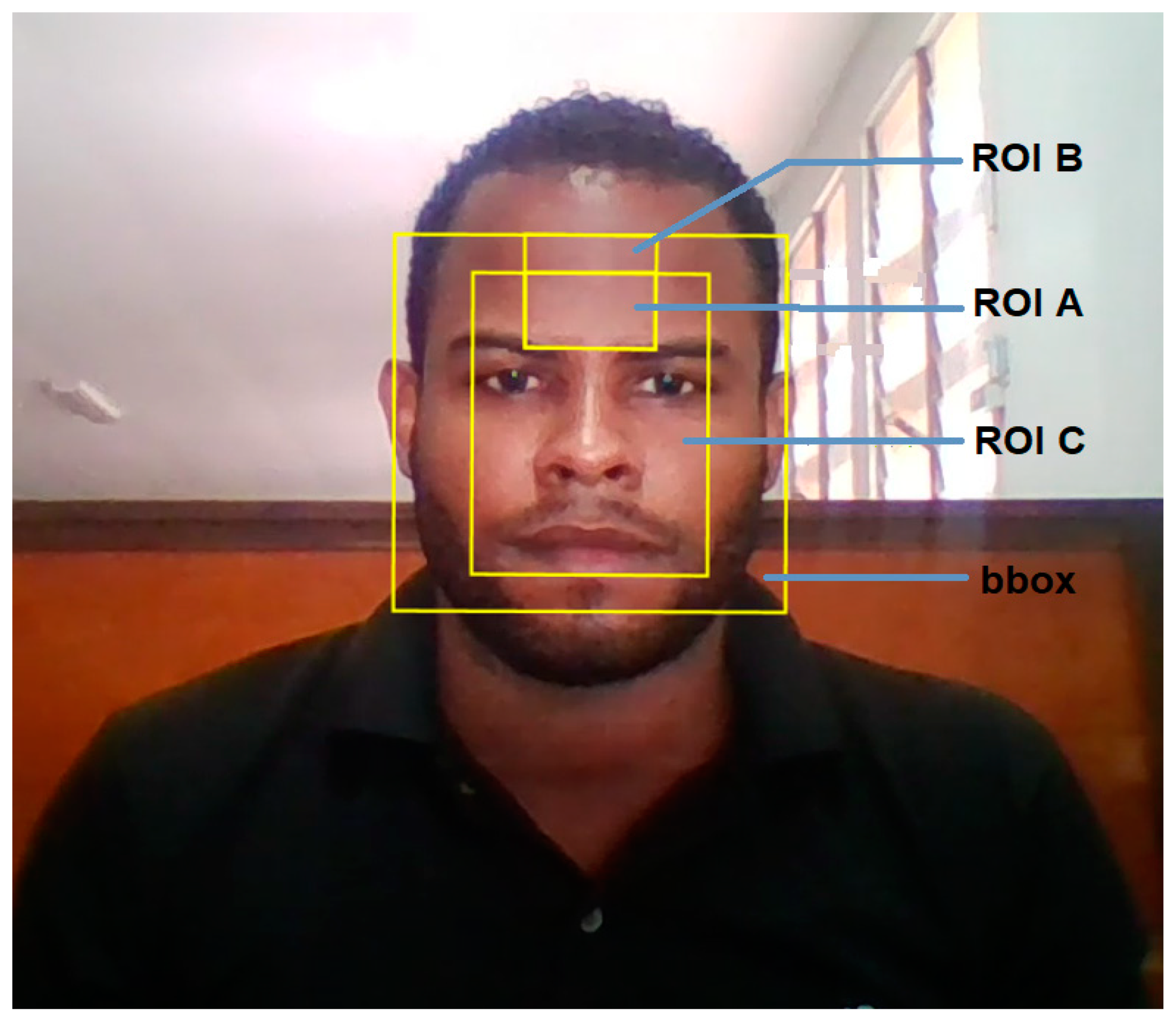
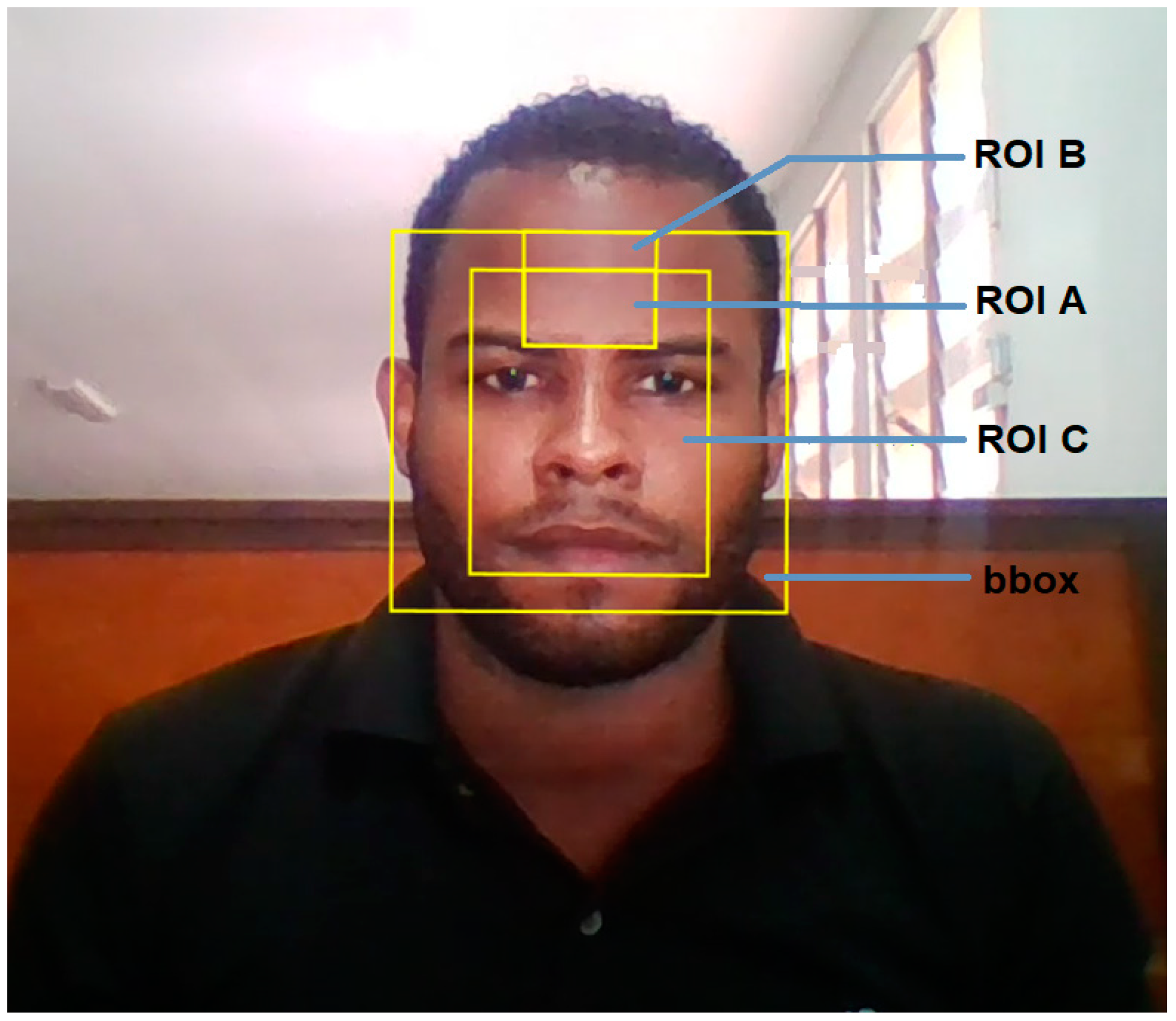
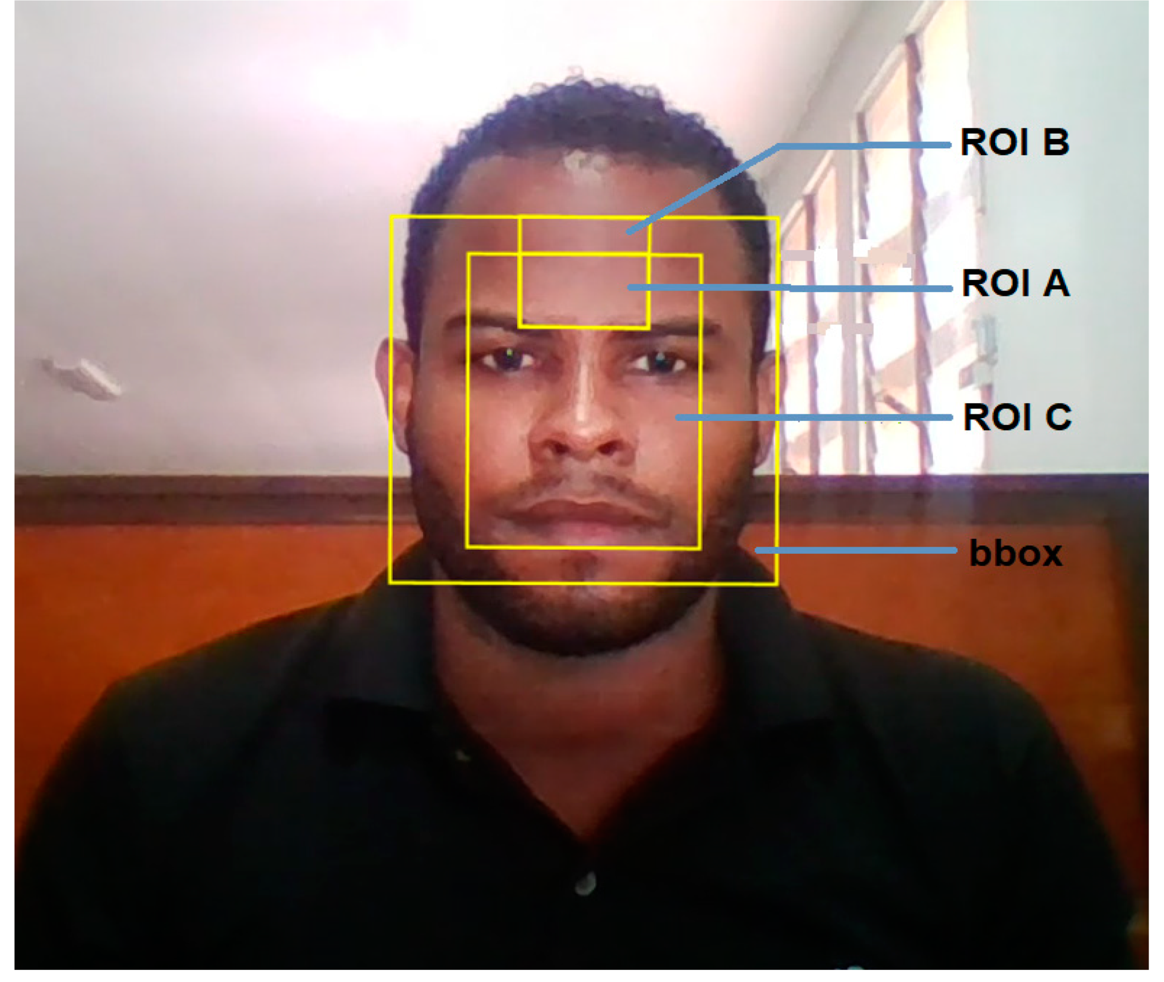
Figure 3.1 shows the various ROIs from which a total of eight (8) different rPPG signals were extracted based on choice of ROI, color space component and spectral analysis technique (FFT or Welch periodogram). For example, two types of signals are extracted from ROI A based on color space – a green signal (RGB color space) and a luminance signal (YCbCr color space). These signals are labelled SIG 1 and SIG 2. They are further distinguished as SIG 1.1, SIG 1.2, SIG 2.1 and SIG 2.2 depending on whether they are processed using the FFT or Welch periodogram. A summarized description of the ROIs and their associated signals is provided in Table 3.1. These designations apply to signals from self-captured videos. Their equivalents for the COHFACE videos are distinguished by “prime” as in the case of SIG 1.1′.
Figure 3. 1. Various ROIs used for rPPG signal extraction. Clarification: ROI B represents the union of ROI A and the small rectangle above ROI A.
Preprints 69042 g005
Table 3. 1. ROI description and rPPG signal classification.
ROI Name ROI Description* Associated Signals Description of Signal
ROI A ROI centred on Forehead
xmin=xmin_bbox+(1/3)*bbox_w
ymin=ymin_bbox+(1/10)*bbox_h
width = (1/3)*bbox_w
height = (1/5)*bbox_h
SIGNAL 1.1 Green (RGB) signal (FFT)
SIGNAL 1.2 Green (RGB) signal (Welch)
SIGNAL 2.1 Luminance (YCbCr) signal (FFT)
SIGNAL 2.2 Luminance (YCbCr) signal (Welch)
ROI B Forehead ROI 50% larger than ROI A
xmin= xmin_bbox+(1/3)*bbox_w
ymin=ymin_bbox
width = (1/3)*bbox_w
height = (3/10)*bbox_h
SIGNAL 3.1 Green (RGB) signal (FFT)
SIGNAL 3.2 Green (RGB) signal (Welch)
ROI C Face ROI comprises central 60% (width) and central 80% (height) of bbox
xmin=xmin_bbox+(1/5)*bbox_w
ymin=ymin_bbox+(1/10)*bbox_h
width = (3/5)*bbox_w
height = (4/5)*bbox_h
SIGNAL 3.1 Green (RGB) signal (FFT)
SIGNAL 3.2 Green (RGB) signal (Welch)
*xmin and ymin refer to the minimum horizontal and minimum vertical pixel positions for the ROI, respectively; xmin_bbox and ymin_bbox are the xmin and ymin for the bounding box of the face detector, while bbox_w and bbox_h are its height and width, respectively.

3.4. Mean Error, RMSE and SNR Definitions

The performance of the rPPG signals were evaluated using two agreement-based metrics – mean error and RMSE – along with the mean SNR. Mean error, RMSE and SNR are mathematically defined as follows:
M e a n   E r r o r   =   1 m i   =   1 m a b s E s t i     R e f i / R e f i
R M S E = 1 m i = 1 m E s t i R e f i ) 2
where Esti and Refi represent the ith estimated and reference HR, respectively and m represents the number of HR values
M e a n   S N R = i = 1 m S i T i S i  
where Si is the sum of spectral components contributing to the ith signal and Ti is the total energy in a spectrum of that signal (obtained by summing all the spectral components); m is the number of signals.
Mean error and RMSE measures for the self-captured videos were based not only on the maximum amplitude frequency peak but also on the signal peak i.e., the peak associated with the HR. The use a signal-peak assessment in addition to the standard maximum-peak assessment was motivated by very low SNR coupled with the observations that:
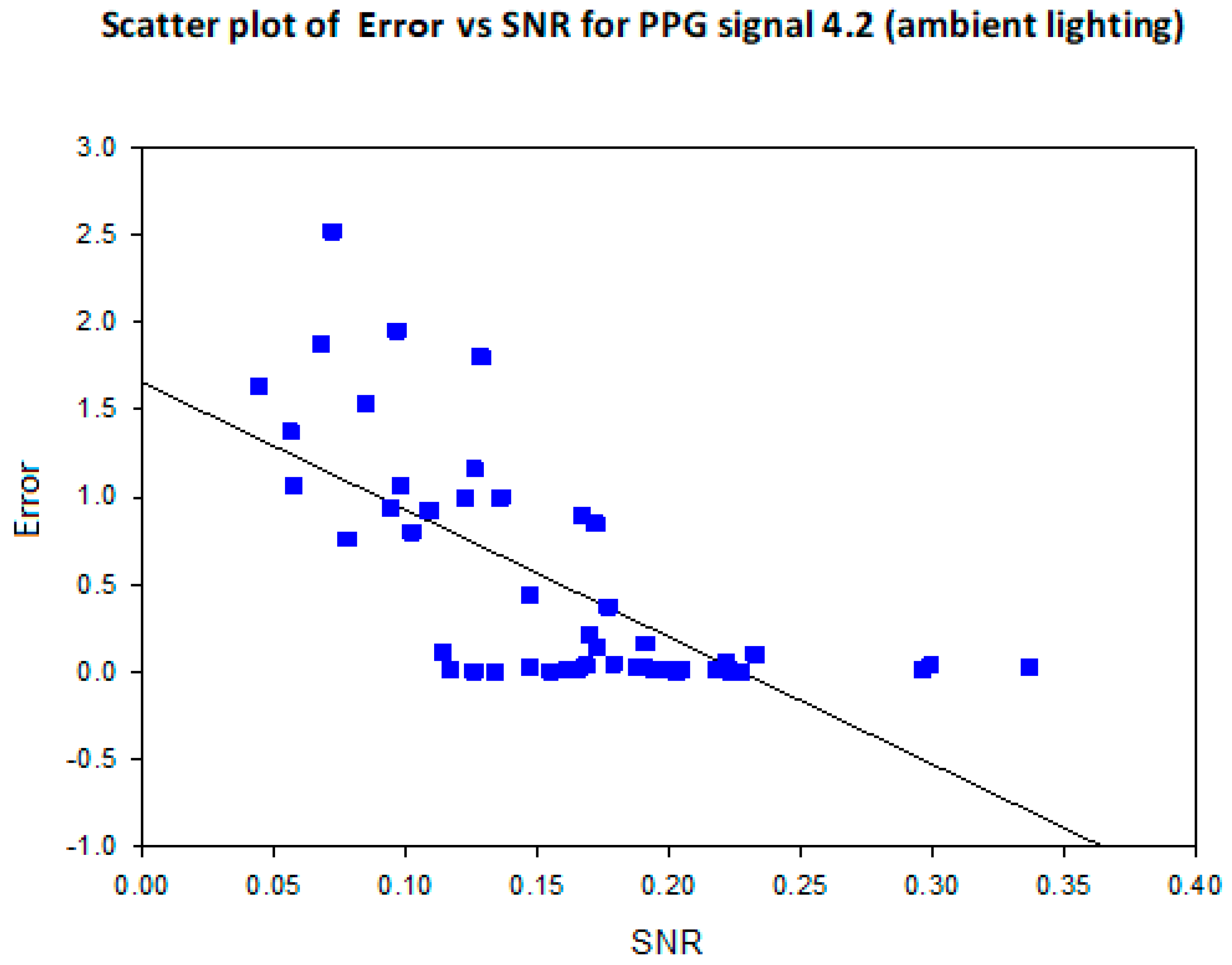
  • error is (negatively) correlated with SNR
  • when the max peak did not correspond to the ground truth HR, a distinct inferior peak which matched the heart rate could most often be seen in the frequency spectrum
This secondary measure afforded a more useful assessment of mean error under low SNR as it approximated what mean error would be like for high SNR signals. There was, however, some uncertainty in signal peak identification in (a few) cases where there was no distinct signal peak. Nevertheless, since most signal peaks were easily identifiable, the advantage of the method outweighed its shortcoming.
A similar problem occurred in the calculation of SNR. While calculating T is straightforward, calculating S is ambiguous because of the stated uncertainty in the determination of the signal peak. There was also the problem of specifying the bandwidth of the signal peak. Generally, the bandwidth of a signal is defined in terms of the full width at half maximum (FWHM) of its main lobe. However, it was observed that the main lobe was often flanked by noisy peaks. In such a case, calculating S translates to summing significantly different frequency ranges, depending on the level of noise flanking the signal peak. To avoid this, a fixed range of ±10 bpm was used for the calculation of S. This is comparable to the method used by Sahindrakar et al. (2011).
Mean error and RMSE evaluation for the COHFACE videos were based exclusively on maximum peak estimates, obviating the need to resolve the problems discussed above for the self-captured videos. However, in 2 (out of 48 cases), SNR was very low and warranted the evaluation of SNR based on a crude estimation of the signal peak location. Like the self-captured videos, the SNR of signals extracted from the COHFACE videos were computed using a value of S summed over a fixed range of ± 10 bpm.

4. Materials And Methods 2: Workflow & Algorithms

This chapter begins with an overview of the thesis workflow and associated algorithms, followed by a step-by-step discussion of the same. It also considers how HR is determined from the processed rPPG signals and offers a simple description of color models and spaces, with particular reference to RGB and YCbCr (the color models used in this thesis).

4.1. Overview of Workflow

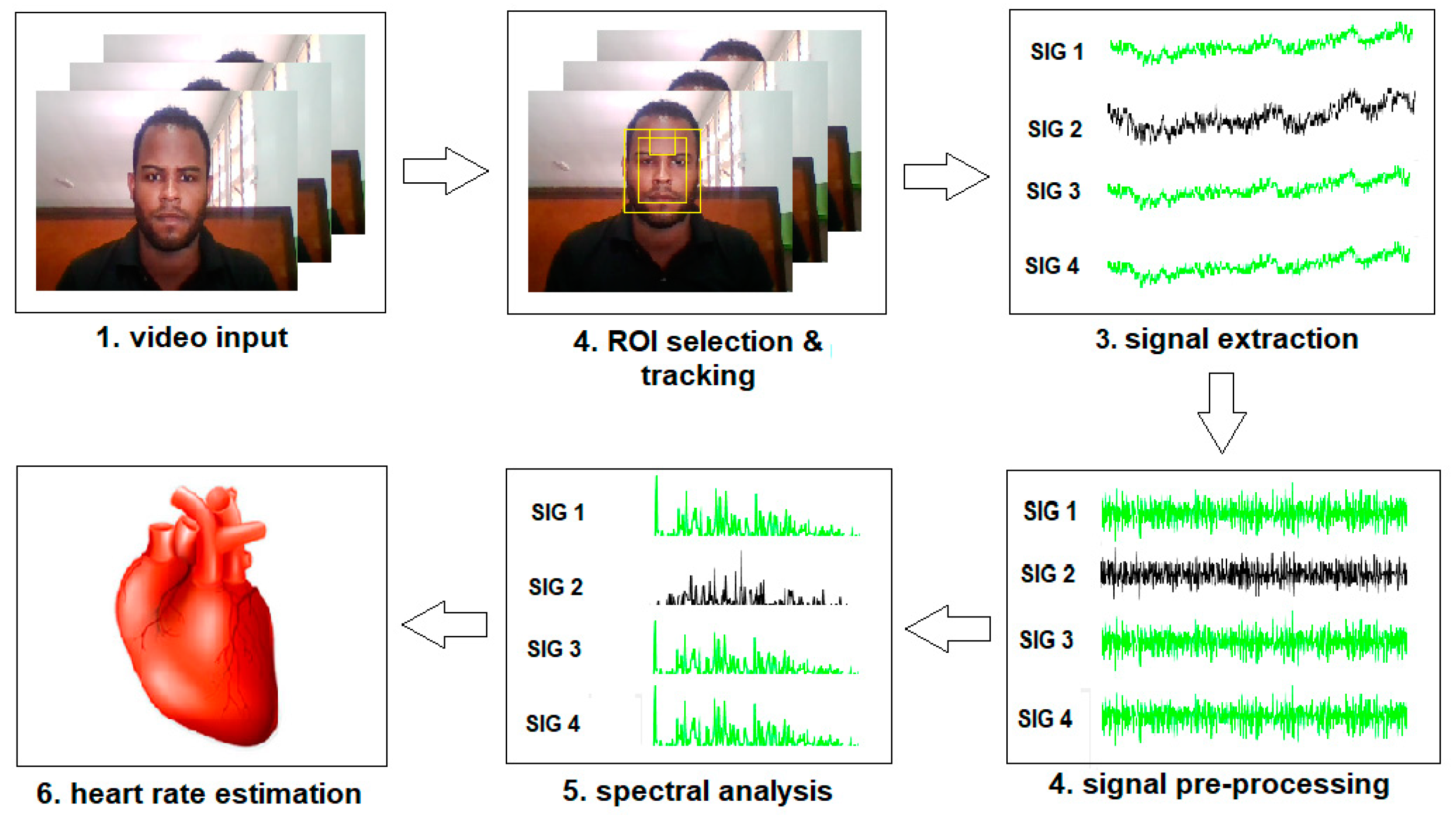
The workflow adopted in this thesis (Figure 4.1) is primarily based on that of Rahman et al. (2016).
Figure 4. 1. Implementation workflow.
Preprints 69042 g006
In the first block, a facial video of the subject is captured by webcam. The video frames are then fed into the next block for facial detection, ROI selection and tracking. Facial detection is performed using the popular Viola-Jones algorithm while tracking employs the equally popular KLT algorithm. A face is detected only in the first frame and is tracked across frames. This is far more computationally efficient than detecting the face in each frame. Three ROIs were investigated in this thesis – forehead ROI A, forehead ROI B (50% larger than ROI A) and ROI C (which covers most of the face). ROI selection is crucial in optimizing SNR. The use of forehead ROIs is based on the discovery by Verkruysse et al. that the forehead yields the strongest rPPG signal (2008). For each frame, the mean pixel intensity of each ROI is calculated for the relevant color component (in RGB or YCbCr space). The mean pixel intensity constitutes a single point in a vector representing the raw rPPG signal. The raw signals are pre-processed in the fourth block via detrending, filtering and normalizing algorithms. The next block converts the pre-processed time-domain signals into the frequency domain using spectral analysis (FFT and Welch periodogram). The HR is taken as the frequency of the component with maximum amplitude.
All algorithms in the workflow were programmed in MathWorks MATLAB® – a numerical computing programming language and integrated development (IDE) environment. By way of toolboxes such as Signal Processing, Image Processing and Computer Vision System, MATLAB is especially suited for signal and image processing.
The following sections of this chapter will delineate the techniques and algorithms in each block and their relevance in implementing research objectives.

4.2. Video Input

The data input for the generation of the raw rPPG signals consisted of the frames of 60-s videos recorded at 29 fps (for self-captured videos) and 20 fps (for COHFACE videos) with a resolution of 720 x 1280 pixels and 640 x 480 pixels, respectively. Videos were stored in MP4 format (for self-captured videos), and AVI format (for COHFACE videos), with 8-bit encoding per colour channel (i.e., 24-bit RGB). The videos were captured by webcam and viewed using the Microsoft Films and TV app. See Section 3.2 for a more comprehensive description of the circumstances of video capture.

4.3. ROI Selection and Tracking

The selection of an appropriate region of interest (ROI) within an input frame is an important preliminary step in reducing the noise in raw rPPG signals extracted from video. Ideally, a ROI contains only skin pixels since only these contain information about the cardiac-synchronous reflectance variations; all other pixels contribute to signal noise. Another advantage of ROI selection is its computational efficiency as it reduces the number of pixels that must be processed. Once a ROI has been selected in the initial frame, it can be tracked across frames – a method that is both efficient and useful in reducing motion artefact. The face has proven an ideal vascularized surface for rPPG signal extraction (Verkruysse, Svaasand, and Nelson 2008). The first step in ROI selection is face detection.

4.3.1. Face Detection

Face detection is a type of object-class detection. In object-class detection, the objective is to identify every instance of an object in an image belonging to a particular class. Typical objects include pedestrians and cars. Face-detection algorithms are most often designed for the detection of frontal human faces. A widely used algorithm is the Viola-Jones face classifier (Viola and Jones 2001), which is the default option for the Cascade Object Detector in MATLAB’s Computer Vision Toolbox. The Viola-Jones algorithm is known for its robustness (very high detection rate), efficiency and utility in real-time applications. It is made up of four main components:
  • Haar-like feature selection
  • Integral image creation
  • AdaBoost training
  • Cascading classifiers
Figure 4. 2. Bounding box of face detected by Viola-Jones algorithm.
Preprints 69042 g007
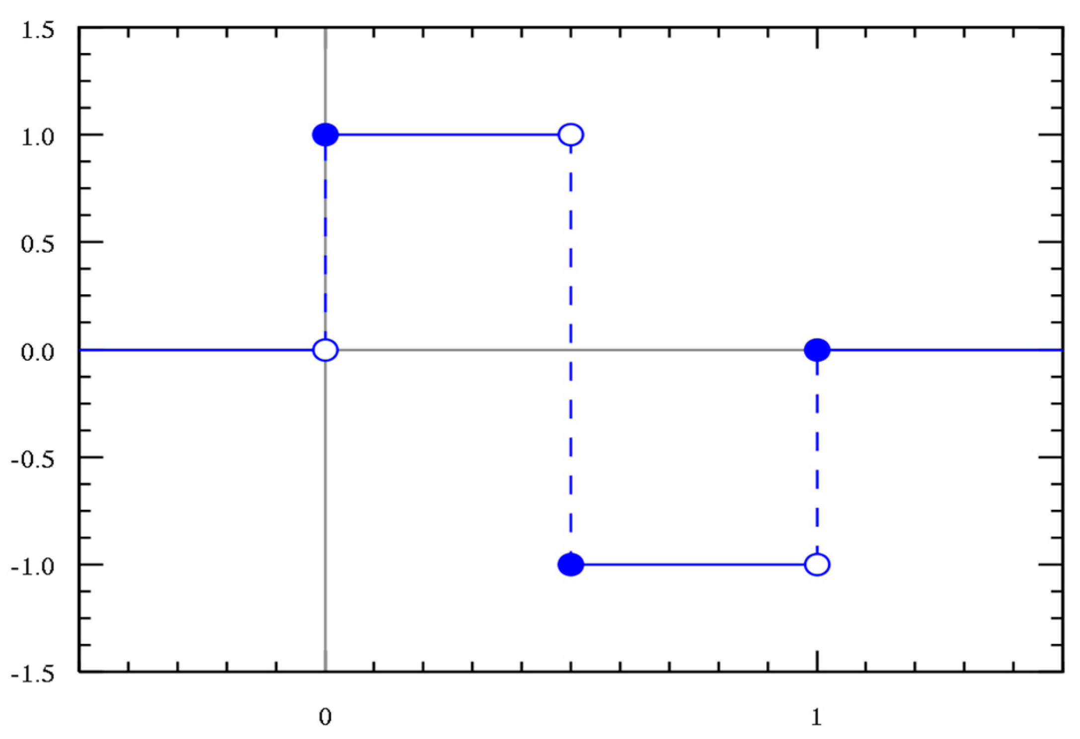
Haar-like features are digital image features used in object detection. They are so named because of their resemblance to Haar wavelets – a series of rescaled square-shaped functions which together comprise a wavelet family.
Figure 4. 3. A Haar wavelet. Wikimedia Commons contributors / CC-BY-SA-3.0.
Preprints 69042 g008
A Haar-like feature can be imagined as a crude approximation of the intensity profile of an image or image sub-window and attempts to capture the essential appearance attributes of an object class. For example, all human faces contain some commonalities which may be matched using Haar-like features. These include:
  • Eye region darker than upper cheeks
  • Nose bridge region brighter than eyes
The use of Haar-like features to evaluate these commonalities is illustrated in Figures 4.4 and 4.5
Figure 4. 4. Haar-like feature that looks like bridge of nose applied to face.
Preprints 69042 g009
Figure 4. 5. Haar-like feature that looks like eye region applied to face.
Preprints 69042 g010
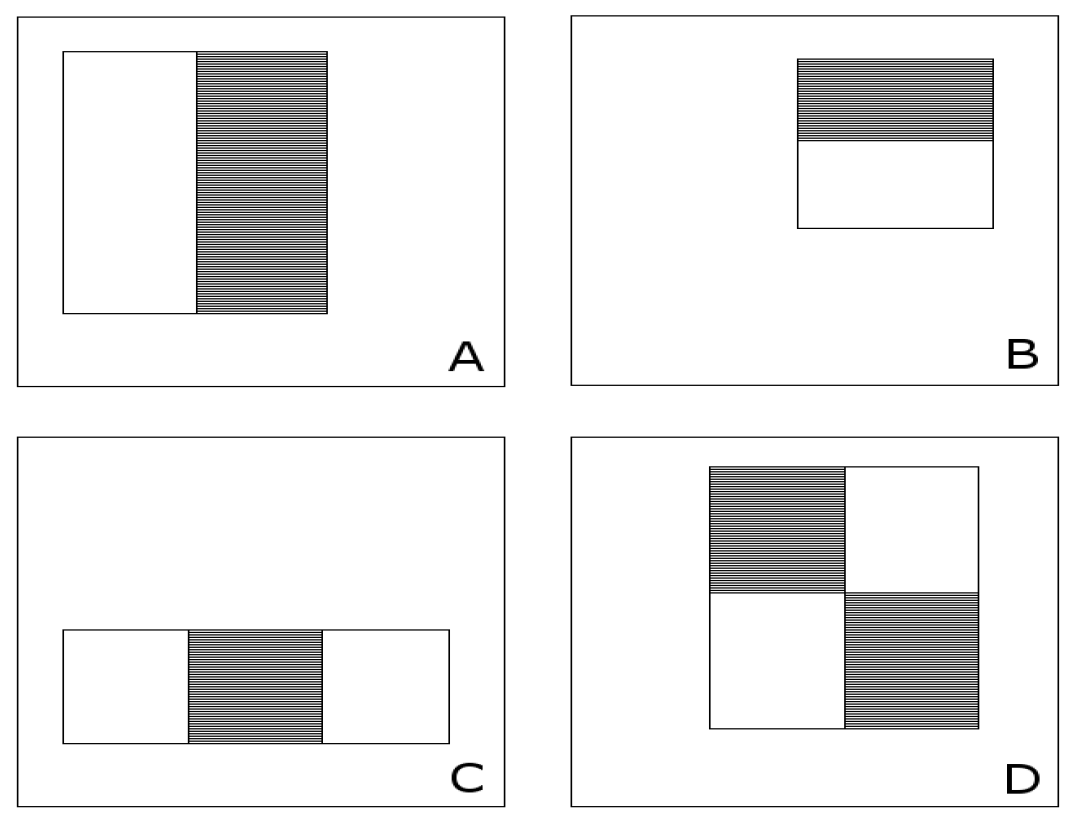
Haar-like feature evaluation is based on the principle of computing the difference between the sum of pixels in adjacent white and black rectangles in an image i.e., value = Σ (pixels in black area) – Σ (pixels in white area). In the original implementation of the Viola-Jones algorithm, feature evaluation was performed on 24 x 24-pixel sub-windows of an image (Viola and Jones 2001). Though the Haar-like features were limited to four types (shown in Figure 4.6), at all possible scales and positions, these features required more than 160,000 evaluations over the sub-window (far more than the number of pixels, which is 24 x 24 = 576). At 160,000 evaluations per sub-window, the summing over pixels required for each feature evaluation is computationally very expensive and of limited use in real-time applications. Viola and Jones proposed an novel solution to this problem by introducing the integral image, more generically known as the summed-area table (Crow 1984).
Figure 4. 6. Haar-like features used in the original implementation of the Viola-Jones algorithm. Prmorgan / Wikimedia Commons / Public Domain.
Preprints 69042 g011
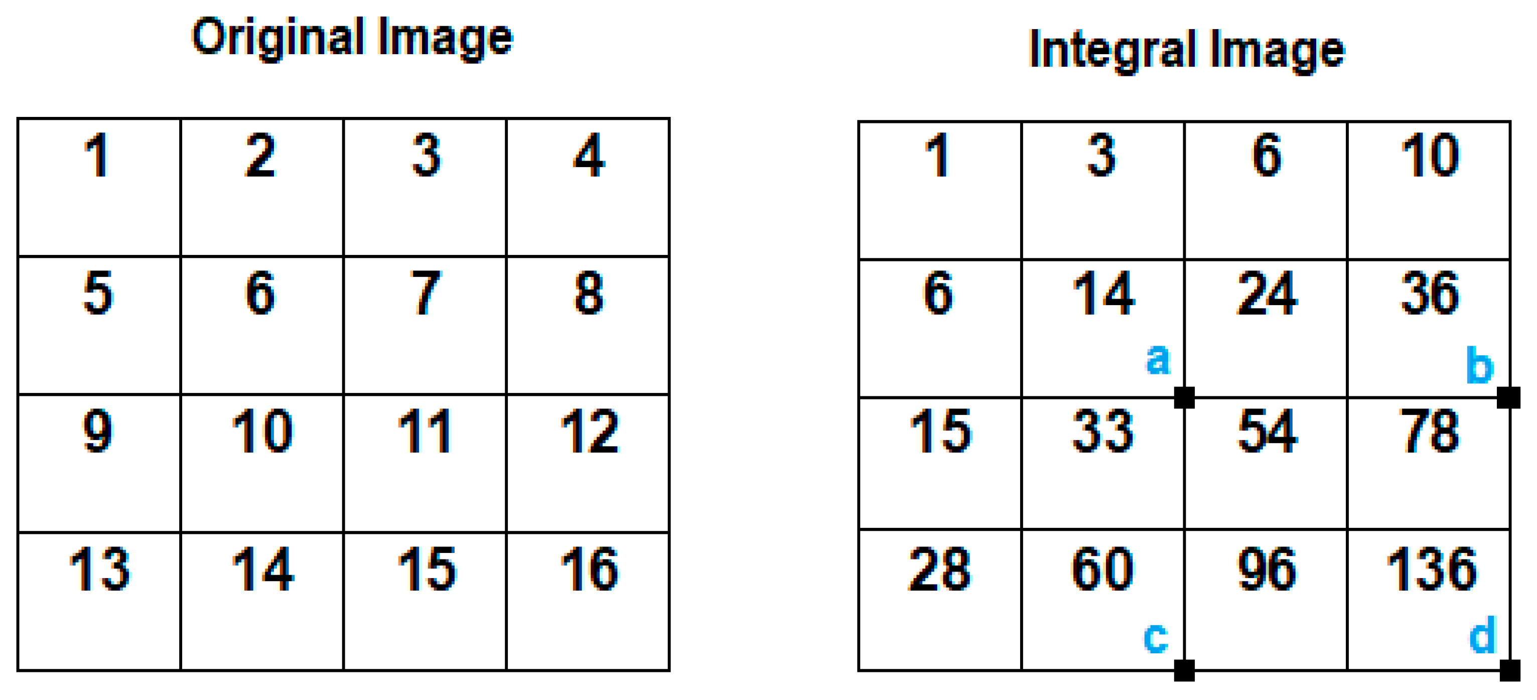
The integral image is a data structure which allows rapid computation of the sum of pixels in an image or image sub-region in constant time. The pixel intensity I(x,y) at any point (x,y) in an integral image is the sum of the intensity i(x,y) of all pixels above and to the left of (x, y), inclusive, in the original image. This may be mathematically expressed as:
I x , y = x '     x ,   y     y i x ' , y '
The integral image can be computed in a single pass over an image since the value I(x, y) in the integral at (x, y) is defined recursively as:
I ( x , y ) = i ( x , y ) + I ( x , y 1 ) + I ( x 1 , y ) I ( x 1 , y 1 )
Once the integral image has been set up, computing the sum of pixels for any rectangular sub-region of an image requires only four references (independent of the size of the sub-region). For a rectangular sub-region defined by coordinates A, B, C, D, the sum of pixels is given by:
x o   x   x 1 , y   y   y 1 ,   i ( x , y )   =   I ( A )   +   I ( D )     I ( B )     I ( C )  
where A=(x0, y0), B=(x1, y0), C=(x0, y1) and D=(x1, y1)
Figure 4. 7. Intensity values of an image and its integral counterpart. I(a) + I(d) – I(b) – I(c) = 20 + 74 – 39 – 33 = 22.
Preprints 69042 g012
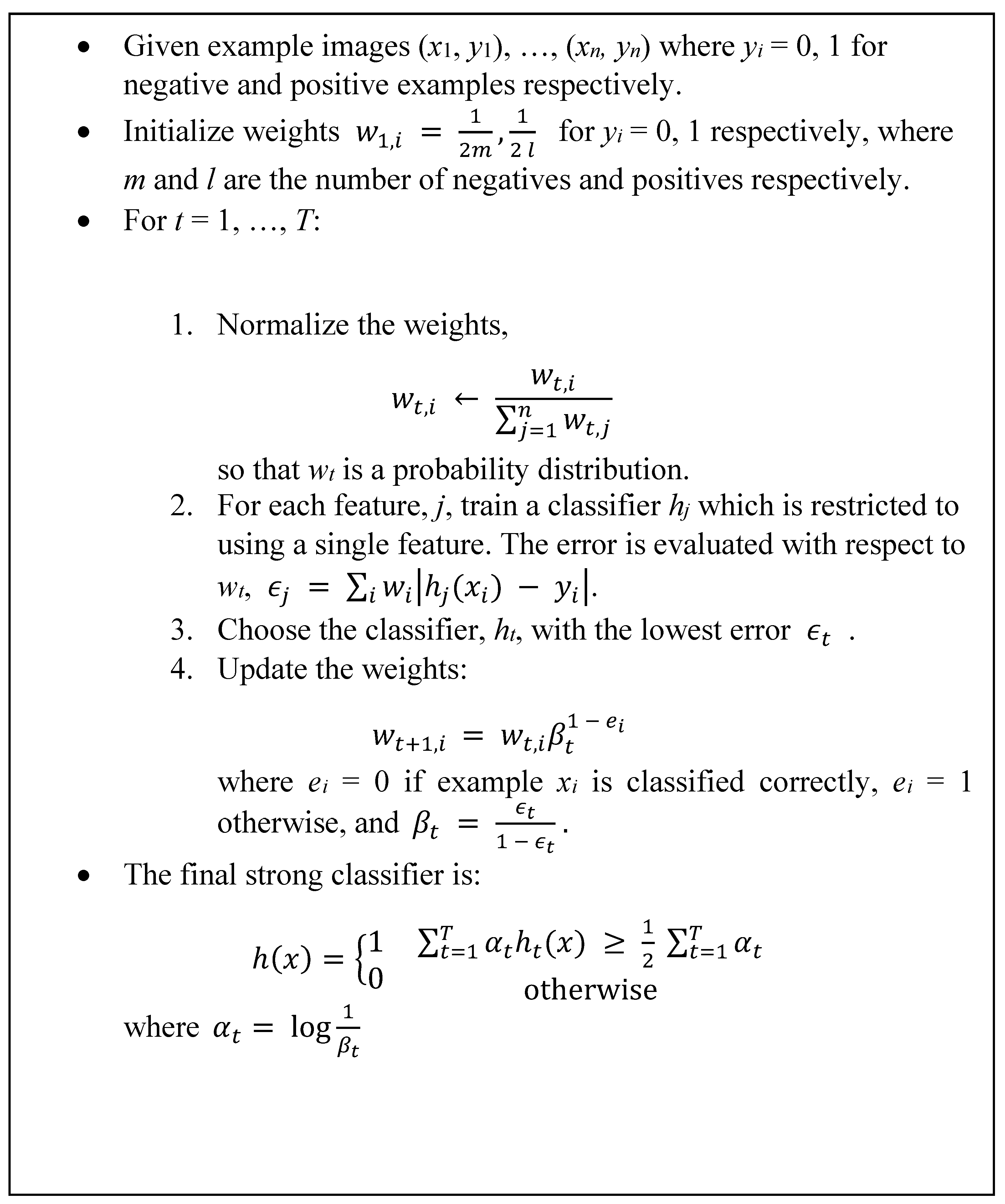
Even with the computational efficiency afforded by the integral image, evaluating 160,000+ Haar-like features for each 24 x 24 sub-window is still computationally prohibitive for real-time facial detection. Most Haar-like features are useless for a given object class. Therefore, a method for selecting the most useful Haar-like features could significantly improve the time complexity of the detector. Viola and Jones achieved this selectivity by using a variant of a pre-existing algorithm known as AdaBoost (Freund and Schapire 1997).
AdaBoost, short for Adaptive Boosting, is an example of a boosting algorithm – a class of machine-learning algorithms than can be used to improve the performance of other so-called weak learner algorithms. Within the Viola-Jones algorithm, Adaboost both identifies the weak learners and constructs a strong learner from a linear combination of weak learners. Each weak learner is based on one of a set of best-performing Haar-like features (i.e., those that yield consistently high detection rates when applied to a face). With a boosting algorithm, the individual weak learners need only perform slightly better than random guessing to converge to a strong learner. A weak learner h(x,f,p,θ) evaluated over a 24 x 24-pixel sub-window x consists of a feature (f), a threshold (θ, which decides whether x is classified as face or non-face) and a polarity (p, indicating the direction of the inequality). Both p and θ are determined during training.
h ( x , f , p , θ ) = 1   0   i f p f ( x ) < p θ   o t h e r w i s e
A strong learner HT (a linear combination of weak learners) selected over T trials of testing may be mathematically defined as:
H T ( x ) = i   =   1 T h i ( x )
where hi represents the ith weak learner in the T trials.
Apart from determining the best Haar-like features, the modified AdaBoost algorithm also sets the polarity and threshold for each weak classifier. There seems to be no satisfactory solution to this problem except brute force i.e., the determination of each new weak classifier in the T trials of testing involves evaluating each feature on all the training examples (at different thresholds and polarity). The best performing feature in a testing trial is the feature which minimizes the weighting error it produces. This weighting error is a function of the weights assigned to the training images. The weight of a correctly classified image is decreased, while that of a misclassified image is kept constant. As a result, the ith feature added to the classifier is forced to “focus” harder on the test images misclassified by the (i – 1) previous features. The weighting system is, therefore, an integral aspect of AdaBoost.
Table 4. 1. Modified AdaBoost algorithm (Viola and Jones 2001).
Preprints 69042 i001
With the integral image and modified AdaBoost, the Viola-Jones algorithm seems ready for facial detection. However, computations thus far have focused on a single 24 x 24-pixel sub-window. Most images have higher resolution, meaning that the Viola-Jones detector would have to evaluate every 24 x 24-pixel sub-window of that image. This is still computationally too expensive and also very inefficient as it is known in advance that most sub-windows contain no face. This calls for a method that can streamline evaluation by discarding sub-windows with no face with minimal computational effort and spending more time on potentially positive windows. Viola and Jones resolved this problem through yet another novel contribution known as the attentional cascade.
An attentional cascade or cascaded classifier is a multi-layered classifier architecture in which each level of the classifier consists of a strong classifier prepared by the modified AdaBoost. The objective at each layer is to determine whether a given sub-window in an image is not a face or possibly a face. A sub-window which fails at any layer is immediately discarded. A simple 2-feature classifier can be adjusted to achieve 100% detection rate with a 40% false positive rate, significantly reducing the number of times the cascade must be evaluated. This classifier can serve as the first layer (or attentional operator) of the cascade, followed by a more complex layer (made up of, say, 10 features) which can perform a stronger evaluation on potentially “harder” negative-windows which survived the first-layer evaluation, and so on. A classifier built on this logic achieves slightly lower detection rates with each successive layer but is compensated by a much faster reduction in false positive rate. This relationship can be evaluated through the detection rate and false positive rate equations below:
Given a trained cascade of K classifiers, the false positive rate F of the cascade is:
F = i   =   1 K f i
where fi is the false positive rate of the ith classifier in the cascade on the examples that it is run on. The detection rate D is:
D = i   =   1 K d i
where di is the detection rate of the ith detector.
As an example, a detection rate of 0.9 and very low false positive rate of approximately 6 x 10⁻⁶ can be achieved by a 10-layer classifier if each layer can achieve a detection rate of 99% (since 0.9 ≈ 0.9910) and a false positive rate of about 30% (0.3010 ≈ 6 x 10⁻⁶).
Figure 4. 8. Schematic depiction of the attentional cascade.
Preprints 69042 g013
Like the weak learners in the boosting stage, cascading classifiers are trained with hundreds of positive and negative samples of the object of interest. In the case of the face, the object of interest in this thesis, training was unnecessary as the MATLAB Cascade Object Detector is pre-trained on a large database of faces.
The process of optimal training of the classifiers in the cascade is not straightforward and requires the solution of an intractable optimization problem. Viola and Jones proposed, instead, a simple framework which nevertheless yields a highly efficient and effective classifier. Under this framework, the user selects the minimum acceptable detection rate and maximum acceptable false positive rate for each classifier. Each layer of the cascade is then trained by AdaBoost with the number of features increased until the target detection and false positive rates are met for that layer. A new layer is added to the cascade until the overall target false positive rate is achieved.

4.3.2. ROI Selection

A face detected by the Viola-Jones algorithm is bounded by a rectangular bounding box (bbox) which contains skin pixels (of the face) and non-skin pixels (in the space surrounding the face). The simplest method of ROI selection sets the modest objective of eliminating non-face pixels by cropping the image to a central fraction of the width and height of the bbox. One recommendation is 60% of the width and 80% of the height (Rahman et al. 2016).
Another method involves the use of a rectangular ROI centred on the forehead. The choice of the forehead as a ROI is based on the discovery by Verkruysse et al. that it provides the strongest rPPG signal (2008). It is also supported by the work of Lewandowska et al. which used thermal images from several subjects to establish the forehead as a particularly uniform region for rPPG signal extraction (2011). Both ROI selection methods were used in this thesis. The positional specifications of the ROIs implemented using the second method are based on the recommendation of Tofighi et al. (2014).
Figure 4. 9. Various ROIs for rPPG signal extraction.
Preprints 69042 g014
Smarter ROI selection methods such as those based on skin detection algorithms are also in use (Kumar, Veeraraghavan, and Sabharwal 2015). These algorithms attempt to take advantage of the higher signal strength associated with larger ROIs, while minimizing the noise contributed by non-skin pixels and the movement on non-rigid facial structures.

4.3.2. Motion Tracking

In the generation of the rPPG signal, it is imperative that the reflectance information be extracted from the same ROI. Inability to maintain this constancy leads to signal noise due to inhomogeneous spatial distribution of skin reflectance. The ideal way of attaining this constancy is by zero relative motion between the subject and camera. However, this is obviously unrealistic, even when attempted, as small variations in the location of the face associated with processes such as breathing and the ejection of blood from the heart (as well as small movements of the camera) invariably lead to error-inducing movements of the ROI. A natural technique for addressing this motional error is to track the movement of the face across frames so that relative motion between the ROI and face is minimized.
Motion tracking could easily be implemented by detecting the face in all frames. However, this is naïve not only because it is computationally inefficient but also because it is prone to significant errors when the face position in a frame is not properly detected.
More robust tracking systems may be designed by calculating the optical flow of image pixels from frame to frame. Optical flow is defined as the pattern of apparent motion of image objects between two consecutive frames caused by the movement of object or camera (Miura et al. 2017). Optical flow is best represented by a 2D displacement vector field in which every vector points from a point in a given frame to an equivalent point in the next frame. Optical flow algorithms may be classed into two categories – dense methods which compute optical flow by considering every pixel and sparse methods which make use of only select pixels. While providing greater tracking accuracy, dense methods are computationally expensive and therefore not viable for real-time applications. A very popular sparse method is the Lucas-Kanade algorithm which limits the optical flow computation to a small subset of image points known as feature points (Lucas and Kanade 1981).
The Lucas-Kanade algorithm is based on three assumptions:
  • brightness constancy – the brightness of each pixel is constant between two consecutive frames.
  • temporal persistence – movements of image objects are small.
  • spatial coherence – neighbouring pixels belonging to a certain surface move in a similar way.
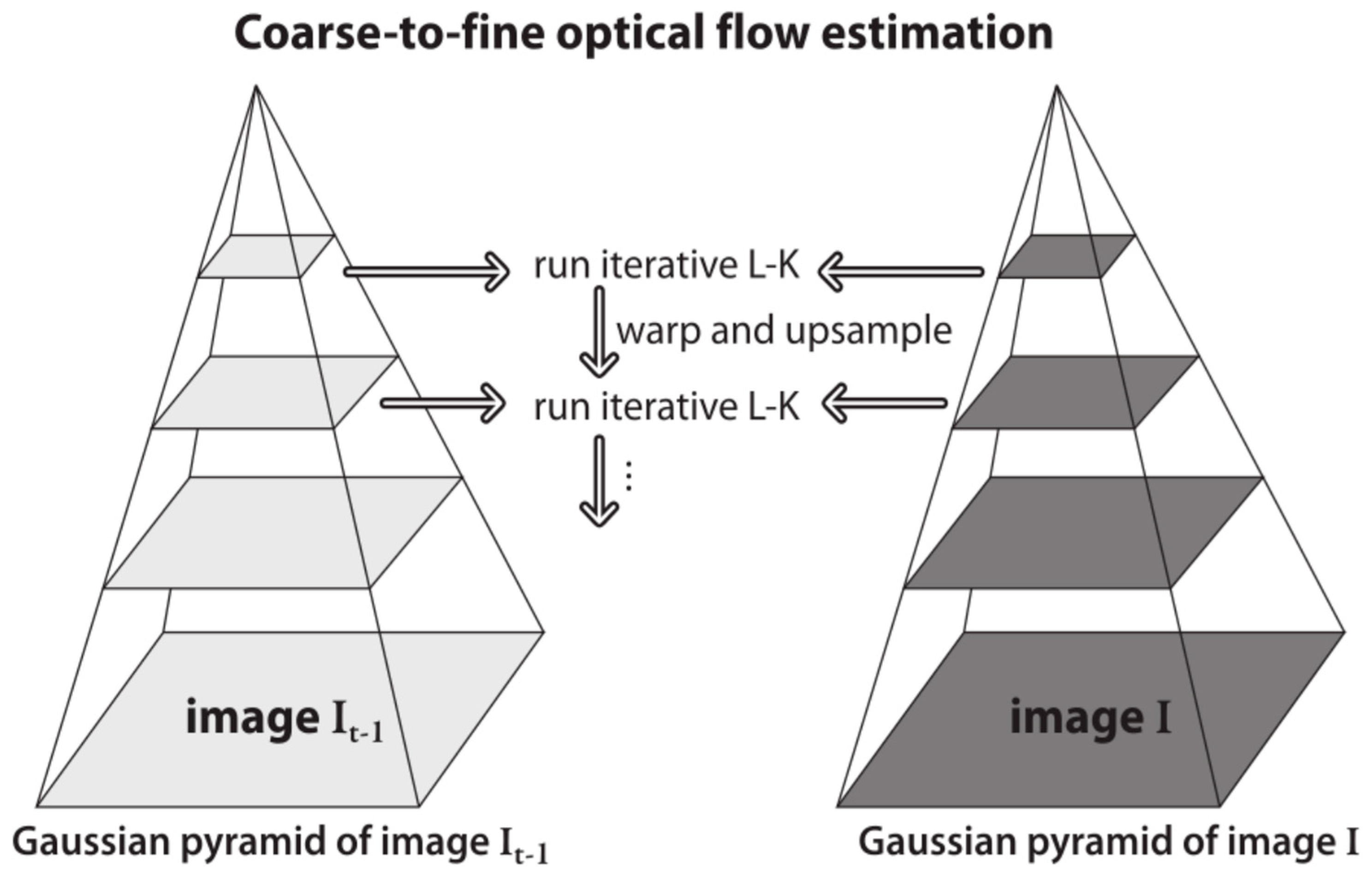
These assumptions are used to construct a system of linear equations describing the optical flow.
Deviation from any one of the three assumptions naturally affects the performance of the algorithm. Large motions, for example, cannot be captured by the optical flow. This limitation has been addressed by Bouguet in a pyramidal implementation of the algorithm (2001). With the pyramids, small motions are eliminated, and large motions are reduced to small motions. The pyramid is constructed by recursive scaling of the resolution of consecutive image frames. The number of frames over which this scaling is done is typically no more than four. If the resolution of the first image is 640 x 480, for example, then that of the next four images will be 320 x 240, 160 x 120, 80 x 60 and 40 x 30.
Figure 4. 10. Schematic depiction of pyramidal implementation of Lucas-Kanade algorithm. Tarasenko et al. (2016). Reproduced with permission from Research India Publications.
Preprints 69042 g015
Even with the motion correction by Bouguet’s pyramid, the Lucas-Kanade algorithm is still far from ideal. This means that the optical flow motion estimation will not always match the actual motion of the subject. This manifests as drift in the ROI position which introduces noise in the associated rPPG signals. Garcia attempted to reduce this error by detected the face every second and readjusting the ROI (2013). However, he also reported that this technique may introduce spurious frequency information in the signal and compromise the accuracy of HR estimation.
Figure 4. 11. Tracking points (white) of the Lucas-Kanade algorithm.
Preprints 69042 g016

4.4. Signal Extraction

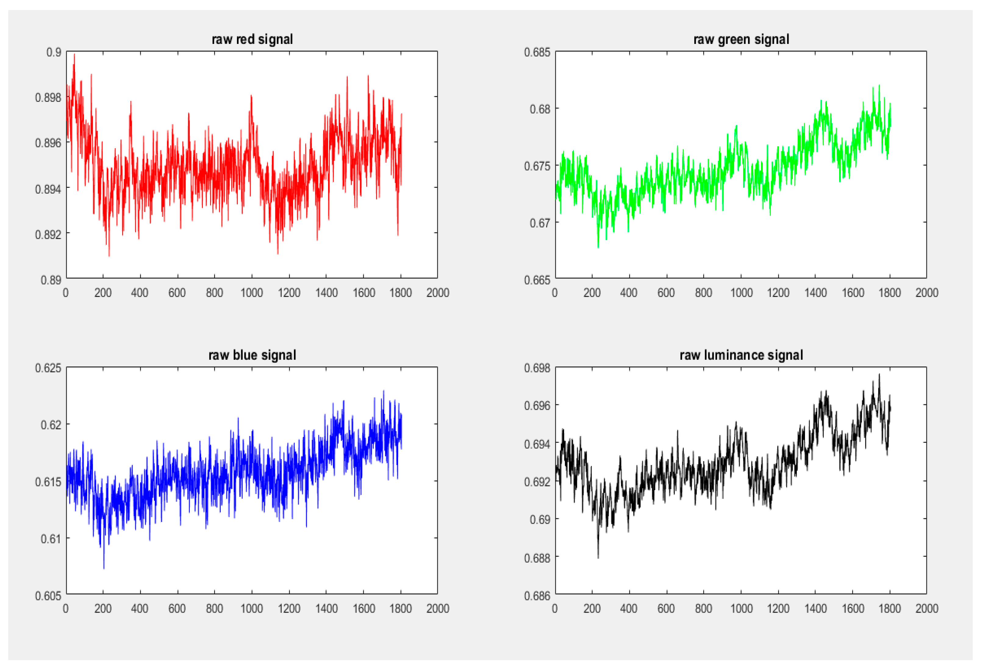
The raw rPPG signal is extracted by averaging the pixel intensity of the ROI for each RGB color channel (or luminance channel, YCbCr) in each input frame. Each mean pixel intensity constitutes one data point in the signal vector and therefore the length of the signal is equal to the number of frames. This rPPG signal is described as raw since it is contaminated with multiple sources of noise which must be reduced before spectral analysis. Noise reduction takes place in the pre-processing stage.
Figure 4. 12. Raw red, green, blue and luminance (Y component of YCbCr) rPPG signals.
Preprints 69042 g017

4.5. Signal Pre-Processing

The purpose of signal pre-processing is to separate out the signal of interest from noise sources in preparation for spectral analysis (or other analytical technique) and HR estimation. The process is not optimal and some noise unavoidably remains in the extracted signal. The first stage of pre-processing is detrending, followed by filtering and normalization.

4.5.1. Signal Detrending

Detrending is used to remove undesirable trends in a signal that may affect its stationarity. A signal is described as stationary if its long-term statistics (such as mean and variance) are relatively invariant in time. Signals typically develop trends through drifting and noising of different kinds. In the case of rPPG signals, this may be caused by changes in physical parameters such as ambient light intensity and temperature. Spectral analysis algorithms typically assume that input signals are at least weakly stationary. The stationarity of an rPPG signal may be significantly compromised in the presence of motional noise. In this research, detrending is performed using the highly recommended smoothness priors approach (SPA), with smoothing parameter λ = 10 and cut-off frequency fc = 0.059 Hz (Tarvainen, Ranta-aho, and Karjalainen 2002). SPA works by removing the low frequency aperiodic trend component from an input signal, leaving behind a nearly stationary signal of interest.
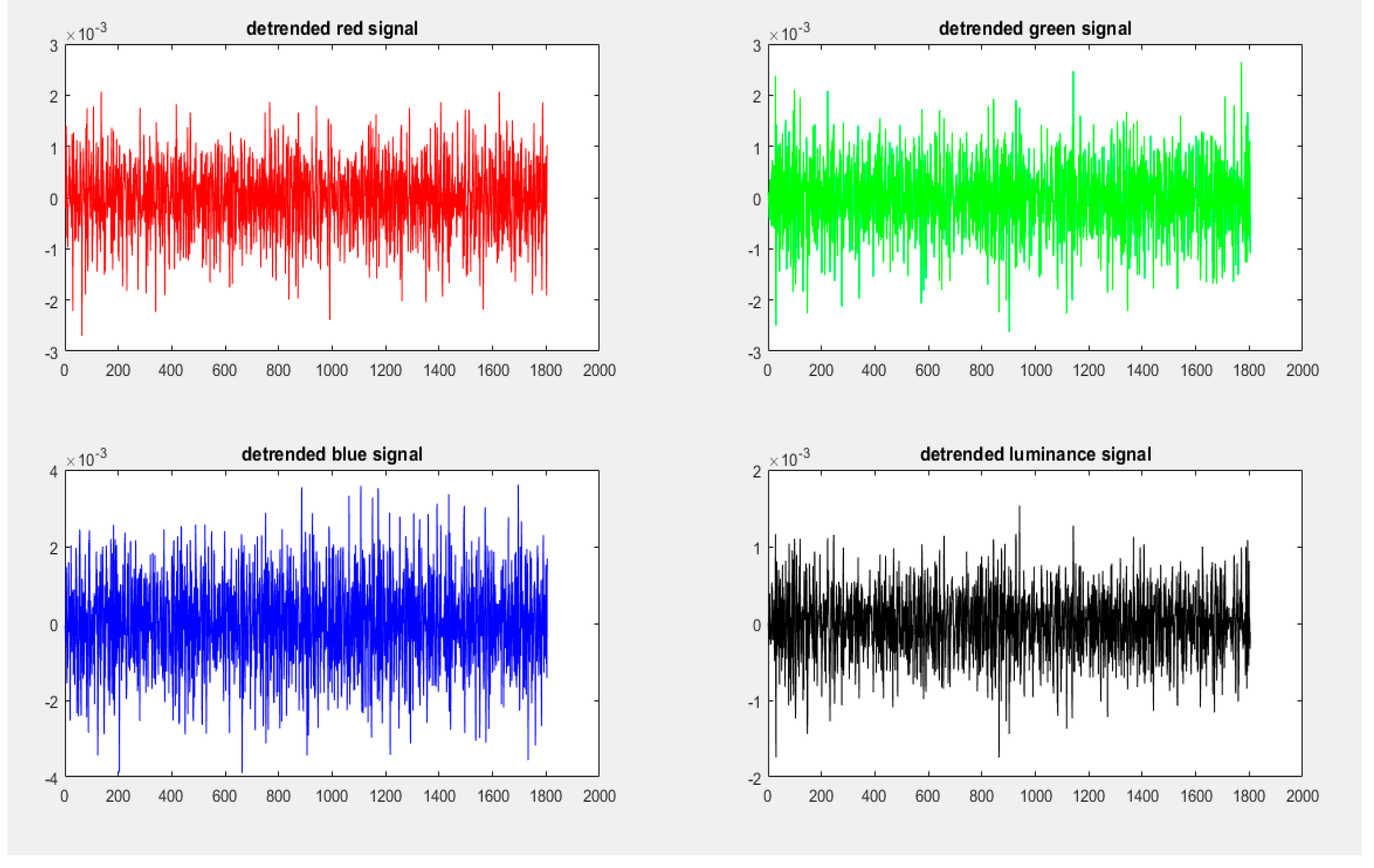
Figure 4. 13. Detrended red, green, blue and luminance rPPG signals.
Preprints 69042 g018

4.5.2. Signal Filtering

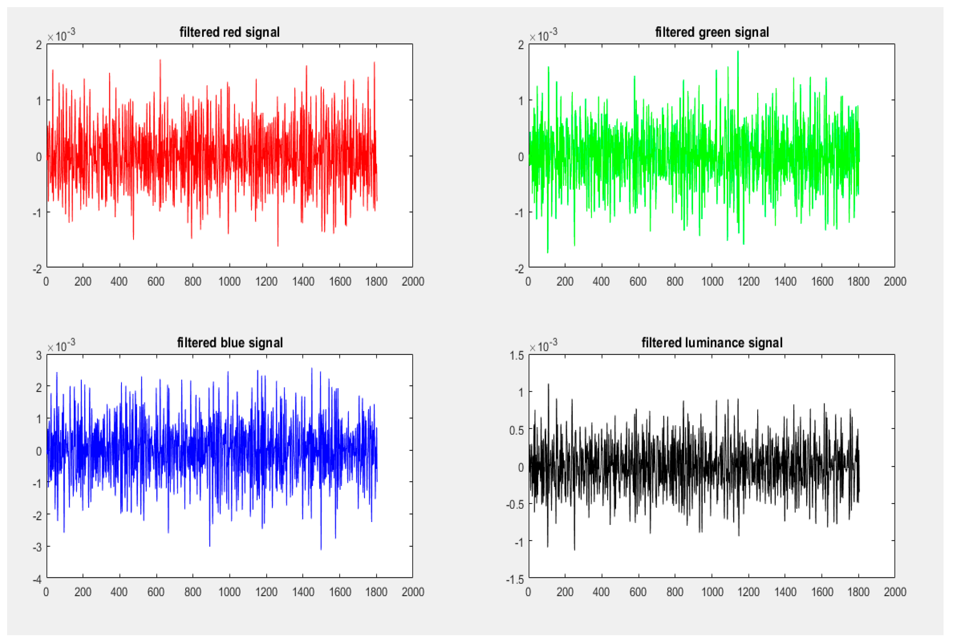
Signal filtering was performed with a fourth-order Butterworth bandpass filter with cut-off frequencies of 0.8 and 6 Hz, following the method of Tarassenko et al. (2014). Signal filtering amounts to a denoising process as it eliminates all frequency components outside the bandpass interval.
Figure 4. 14. Filtered red, green, blue and luminance rPPG signals.
Preprints 69042 g019

4.5.3. Signal Normalization

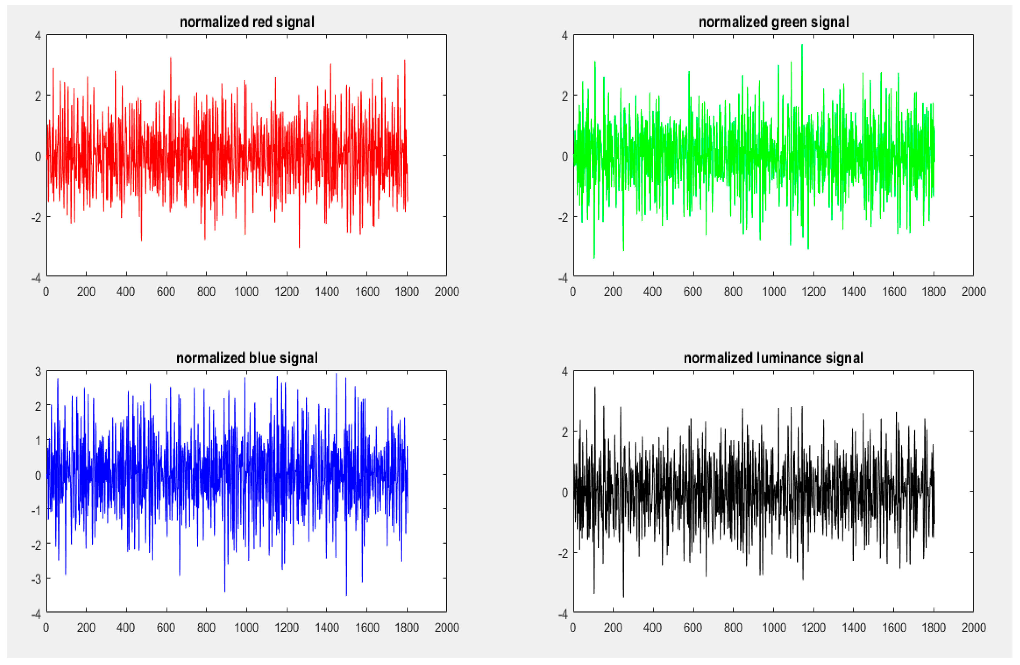
The last stage of pre-processing normalizes all signals of interest to zero mean and unit variance according to the method mentioned by Cochran (1988). The normalized signal Xi given by:
X i ( t )   =   Y i ( t )     μ i δ i  
for each i = R, G and B signals where μ𝑖 is the mean and 𝛿𝑖 is the standard deviation of signal 𝑌𝑖.
Apart from establishing signal comparability, normalization improves algorithmic stability and is a necessary preparatory step for signal processing by procedures such as PCA and correlation analysis.
Figure 4. 15. Normalized red, green, blue and luminance rPPG signals.
Preprints 69042 g020

4.6. Spectral Analysis

An intuitive approach for HR estimation would be counting the number of peaks in the time-domain rPPG signal. However, this method is error prone for several reasons, primarily:
  • spurious peaks presented by the low frequency quasi-DC component of the rPPG signal (it is the AC component which contains the signal of interest)
  • spurious peaks created by residual noise left after the denoising of the pre-processing stage
These problems are either eliminated or minimized in the frequency domain and therefore HR estimation is best handled by spectral analysis.

4.6.1. Fast Fourier Transform (FFT)

The Fourier Transform is a popular method for spectral analysis i.e., the conversion of a signal from the time domain to a representation in the frequency domain. The Fourier transform may be continuous or discrete. Since the rPPG represents a discrete signal, Fourier analysis of the rPPG signal employs the discrete Fourier Transform (DFT).
FFT refers to a class of algorithmic implementations of the DFT. While a naïve (direct from definition) implementation of the DFT has time complexity O(n2), FFT implementation has complexity O(nlogn) and is the most efficient known method for implementing the DFT (Cochran et al. 1967). The DFT is defined by the formula:
X k = n   =   0 N 1 x n e i 2 π k n / N  
where Xk represents a set of complex numbers of cardinality k, xn represents the input signal of length N, and k = 0, …, N – 1.
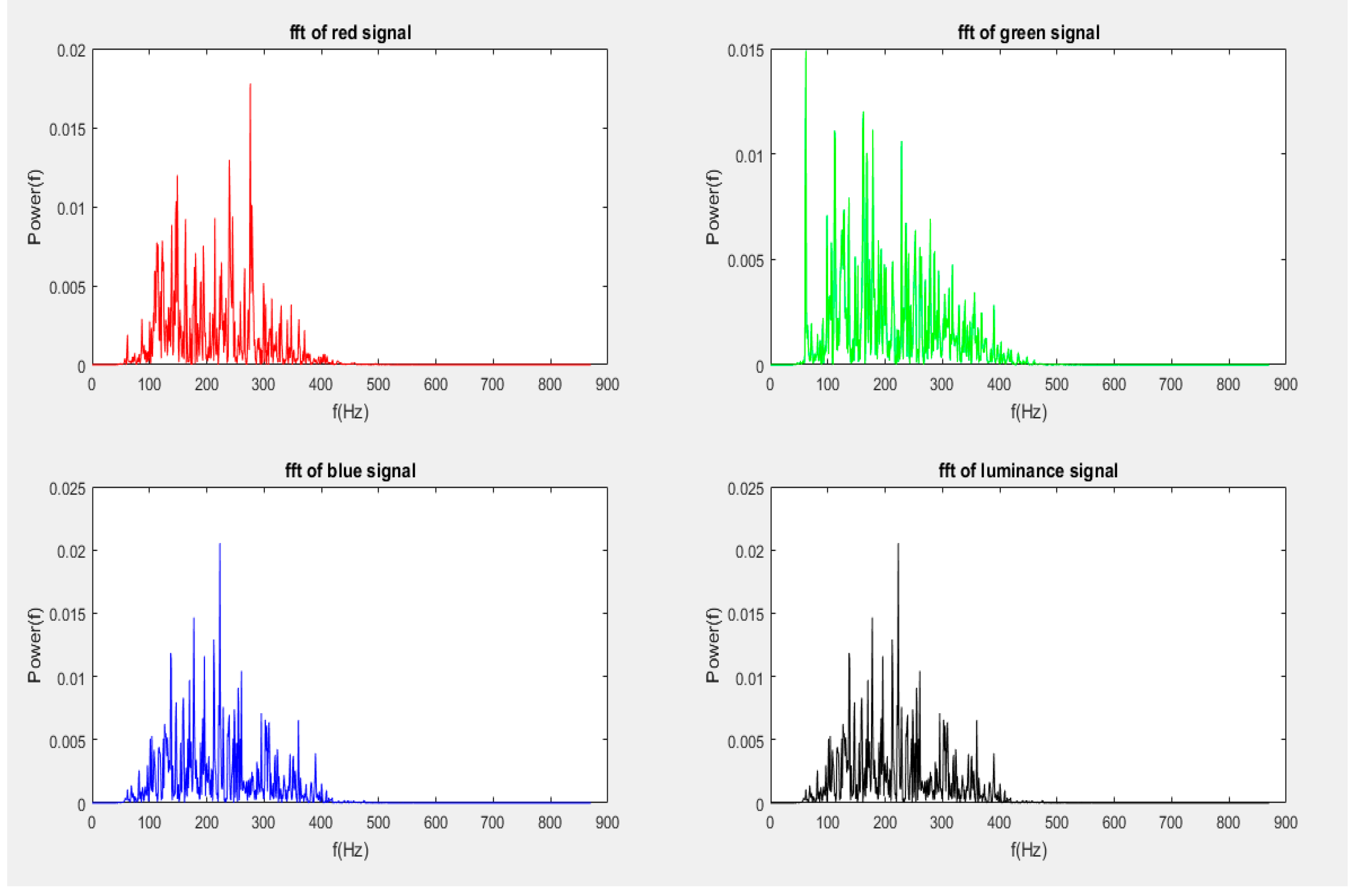
In this thesis, the FFT was implemented using the directly available MATLAB function.
Figure 4. 16. FFT of red, green, blue and luminance rPPG signals.
Preprints 69042 g021
The FFT operates on the assumption that the input signal is periodic and is therefore sensitive to discontinuities at signal end points. In the frequency domain, discontinuities translate to the problem of spectral leakage in which the power of the actual frequency is leaked to surrounding frequencies. Leakage can be reduced by minimizing discontinuities (while preserving frequency information). This can be achieved by windowing in which a function is applied to the signal to produce a smoothed redistribution of amplitude with end points equal to zero.
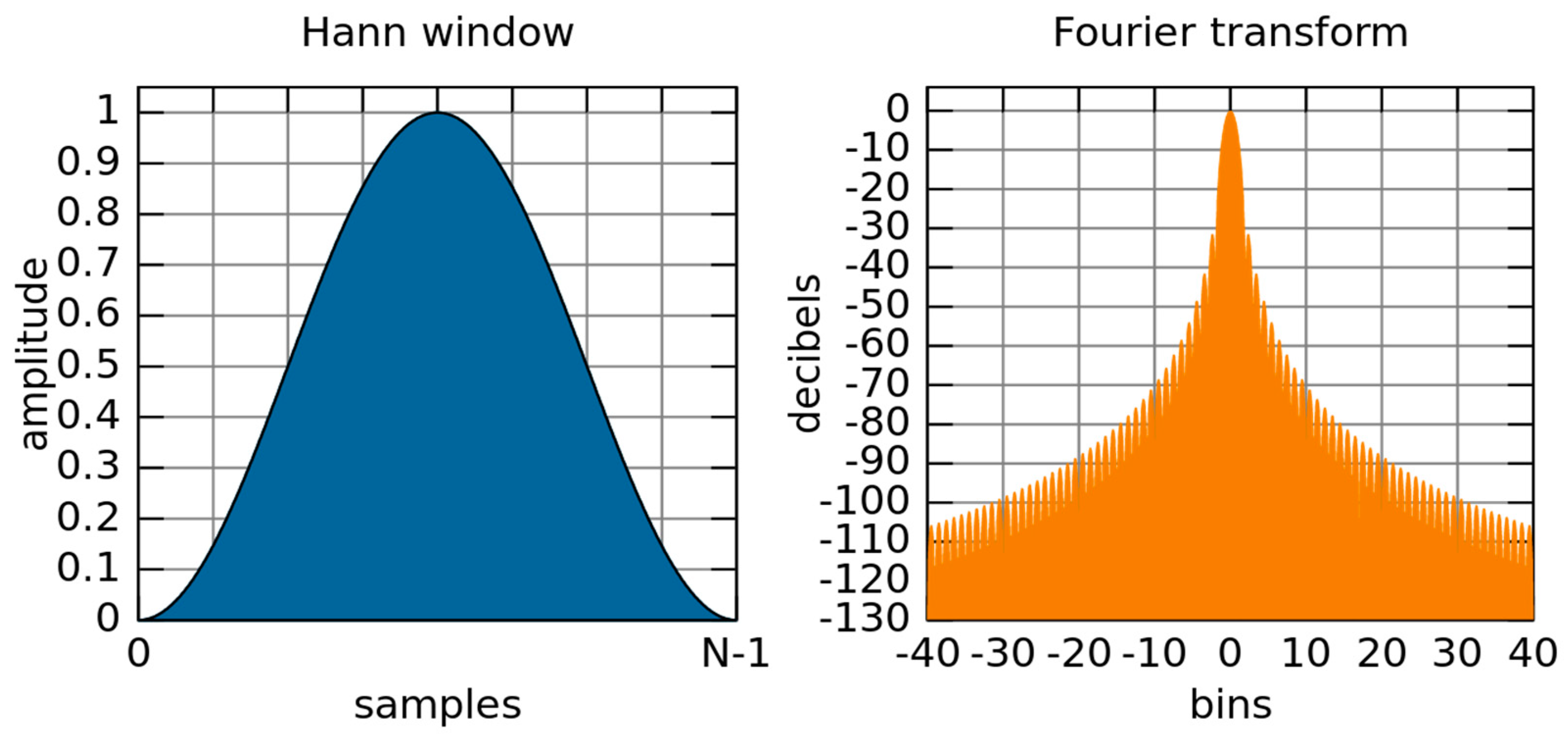
The window function employed in this thesis is the Hann window (depicted in Figure 4.18). This window combines acceptable frequency resolution with moderate spectral leakage. Alternative window functions such as the Blackmann and Blackmann-Harris, though better at reducing spectral leakage, do so at the cost of frequency resolution. The Hann window is highly recommended for general-purpose applications where the nature of the signal is unknown. The mathematical definition of the Hann window (of length N) is given by:
w ( n )   =   1 2 1   c o s 2 π n N     1    
where n = 0, …, N – 1.
Figure 4. 17. Hann window function (left) and its Fourier transform (right). Olli Niemitalo / Wikipedia Commons / Public Domain.
Preprints 69042 g022

4.6.2. Welch Periodogram

A second spectral analysis technique employed in this thesis is the Welch periodogram. It is an implementation of the Fourier transform optimized for unevenly sampled signals and periodic signals of different shapes. The Welch periodogram is an improvement over the standard periodogram as well as Bartlett’s periodogram. Bartlett’s periodogram – also known as the method of averaged periodograms – operates by calculating the average of a series of periodograms derived from non-overlapping segments of an input signal. Its advantage over the standard periodogram is that it reduces signal noise at the cost of frequency resolution. Welch’s method modifies Bartlett’s by averaging over a set of periodograms obtained from overlapping segments of in input signal, yielding greater noise reduction. The procedure for the Welch periodogram involves:
  • splitting of signal into overlapping segments
  • windowing of overlapped segments in the time domain
  • computing of periodograms for individual segments by FFT, followed by squaring of the magnitude
  • averaging of individual periodograms (resulting in the reduction of the noise/variance in the power of the frequency components)
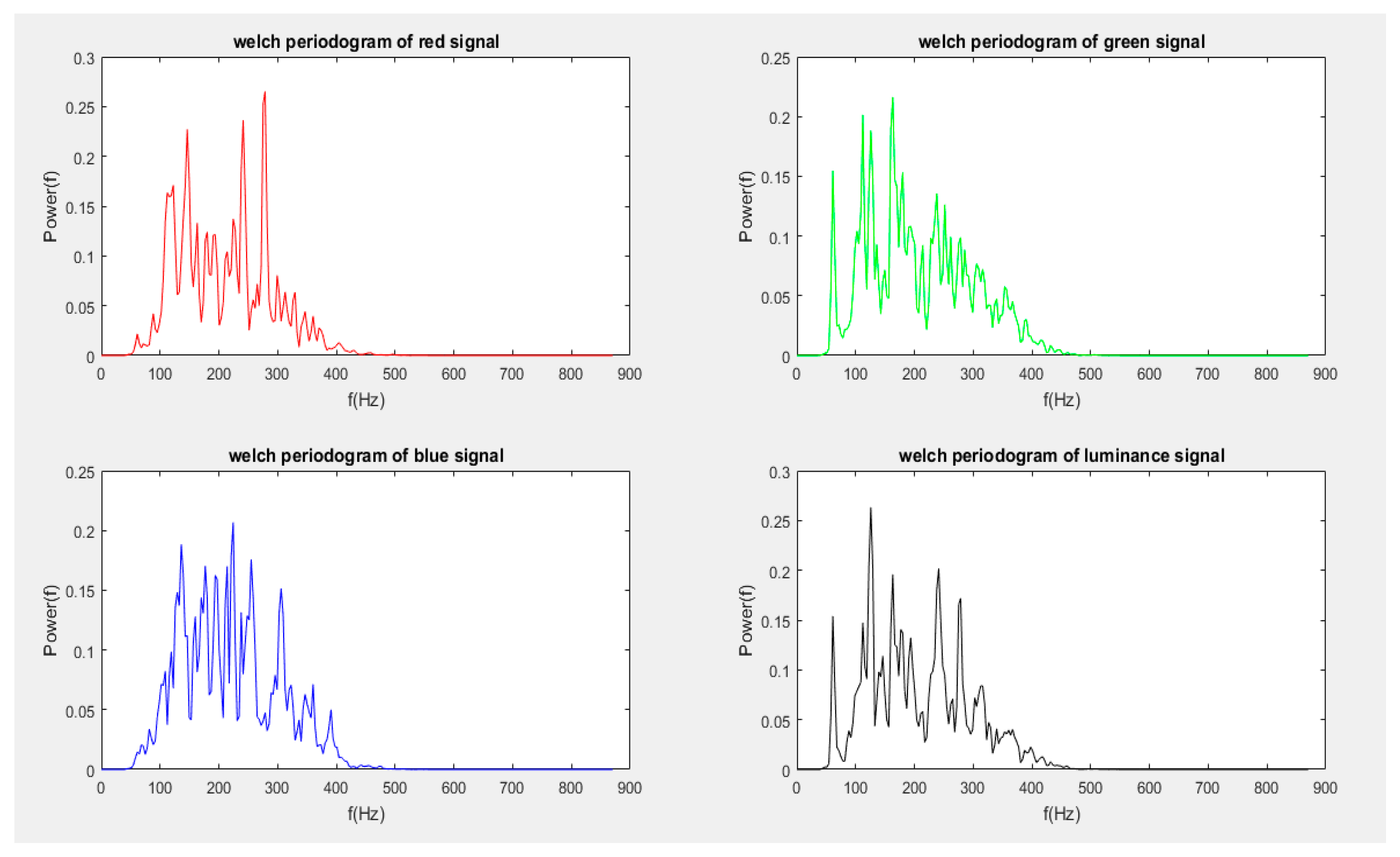
Figure 4. 18. Welch periodogram of red, green, blue and luminance rPPG signals.
Preprints 69042 g023

4.6.3. Summary Autocorrelation Function (SACF)

Autocorrelation, as the name implies, is the correlation of a signal with a delayed/lagged copy of itself as a function of the delay. The correlation measure used in autocorrelation is the Pearson correlation. Autocorrelation is important in signal processing for finding periodicities in noisy signals as correlation peaks occur at lags corresponding to signal harmonics.
Summary autocorrelation is a technique conventionally used in speech processing for identifying fundamental frequencies. The summary autocorrelation function (SACF) is the vector sum of the autocorrelation function of a signal across a range of frequencies (the bandpass in this case) (Bernstein and Oxenham 2005, Brown et al. 2006). The SACF conveniently exhibits peaks at the period of each fundamental frequency (Raghi and Lekshmi 2016).
In this thesis, it was hypothesized that the technique could produce a similar effect for rPPG signals (where harmonics may significantly contribute to signal noise).

4.7. Heart Rate Determination

In this thesis, HR is determined by spectral analysis of the rPPG signals using the FFT and Welch periodogram. Spectral analysis represents the time-domain signals in terms of their frequency components. The HR is taken as the frequency of the component with the highest power. HR (in bpm) is related to frequency (in Hz) by the simple relation:
H R   i n   b p m = 60 f r e q u e n c y   ( i n   H z )
For this implementation, frequency is constrained to the interval [0.8, 6.0] Hz by a bandpass filter. This interval encompasses the range of realistic heart rates in humans.

4.8. Color Models and Spaces

This investigation employed two color models – the RGB model and (the luminance component of) the YCbCr model. A color model is an abstract formal/mathematical description of the representation of colors as tuples of typically three or four elements. The particularization of a color model to a specific interpretation of tuple components is known as a color space. For example, within the RGB color model, there are several color spaces (Adobe RGB, sRGB etc.)

4.8.1. RGB Color Model

The RGB color model is an additive color model in which the primary colors red, green and blue light are combined in various intensity weightings to yield a wide range of secondary colors. The RGB model is widely used for sensing, representing and displaying images in modern electronic devices such as TV and computers, though its theory – based on human color perception – long preceded modern electronics.
In this research, the green rPPG signal was of primary importance as seminal research by Verkruysse et al. (2008) divulged it to yield the strongest rPPG component. Signals derived from the other components – red and blue – were also stored for future analysis aimed at verifying the discovery that a signal X with higher SNR than the green signal can be obtained by combining the R, G and B traces in the mathematical relation: X = R – G + 2B (Sahindrakar, de Haan, and Kirenko 2011).

4.8.2. YCbCr Color Model

YCbCr is a family of color spaces commonly used as a color option in digital photography and video. Y stands for the luminance (approximately brightness) while Cb and Cr are the blue-difference and red-difference chroma components (chroma is approximately equivalent to the concept of hue) A key difference between the RGB and YCbCr models is that the YCbCr isolates brightness to the luminance component and hue to the chroma components while both hue and brightness are simultaneously stored in the in each of the three components of RGB.
In this thesis, in addition to traces from each of the three RGB components, a signal trace was generated from the Y component of YCbCr. The primary motivation for such a signal was to investigate whether there was any advantage in using a component based purely on brightness given that the rPPG signal is based primarily on light intensity variations.
The YCbCr color space may be mathematically derived from the RGB color space using the following transformations (Poynton 2012):
Y = 16 + 65.481 R 256 + 128.553 G 256 + 24.966 B 256
C b = 128 37.797 R 256 74.203 G 256 + 112 B 256
C r = 128 + 112 R 256 93.786 G 256 18.214 B 256

5. Results

This chapter presents the results of the rPPG investigation. Results are classified into two main groups:
  • results for self-captured videos
  • results for COHFACE videos
For self-captured videos, results are further classified based on whether videos were captured in ambient or dedicated lighting and whether HR determination was based on maximum peak or signal peak estimates. For the COHFACE videos, results are further classified based solely on whether videos were captured in ambient or dedicated lighting (since all HR estimates were based on maximum peaks).

5.1. Self-Captured Videos

Mean error (and RMSE)2 of HR estimates were generally poor for self-captured videos. The worst performance was obtained for max peak estimates under ambient lighting, with Table 5.1 showing a mean error range of 50% to 119%. Significant improvement was achieved for signal peak estimates (under the same lighting), with all eight (8) rPPG signals showing a mean error of 2% (Table 5.2).
Table 5. 1. Mean error and RMSE of HR estimates (max peak, ambient lighting).
SIG1 SIG2 SIG3 SIG4
FFT Welch FFT Welch FFT Welch FFT Welch
Mean Error 1.13 0.95 0.75 0.63 1.13 1.19 0.62 0.50
RMSE 124.40 105.00 93.67 76.16 122.60 126.70 83.33 71.08
Table 5. 2. Mean error and RMSE of HR estimates (signal peak, ambient lighting).
SIG1 SIG2 SIG3 SIG4
FFT Welch FFT Welch FFT Welch FFT Welch
Mean Error 0.02 0.02 0.02 0.02 0.02 0.02 0.02 0.02
RMSE 2.54 2.49 2.54 2.49 2.59 2.49 2.49 2.42
Under dedicated lighting, mean error of max peak estimates of HR ranged from 22% to 61% (Table 5.3). This represents an approximately two-fold improvement compared to the ambient lighting case. As with the case for ambient lighting, under dedicated lighting, signal peak estimates of HR showed marked improvement relative to max peak estimates, with all eight (8) rPPG signals showing a mean error of 3% (Table 5.4).
Table 5. 3. Mean error and RMSE of HR estimates (max peak, dedicated lighting).
SIG1 SIG2 SIG3 SIG4
FFT Welch FFT Welch FFT Welch FFT Welch
Mean Error 0.57 0.48 0.39 0.39 0.55 0.61 0.25 0.22
RMSE 78.55 69.55 61.24 60.59 77.46 84.30 49.28 45.45
Table 5. 4. Mean error and RMSE of HR estimates (signal peak, dedicated lighting).
SIG1 SIG2 SIG3 SIG4
FFT Welch FFT Welch FFT Welch FFT Welch
Mean Error 0.03 0.03 0.03 0.03 0.03 0.03 0.03 0.03
RMSE 3.41 3.70 3.43 3.57 3.34 3.37 3.42 3.76
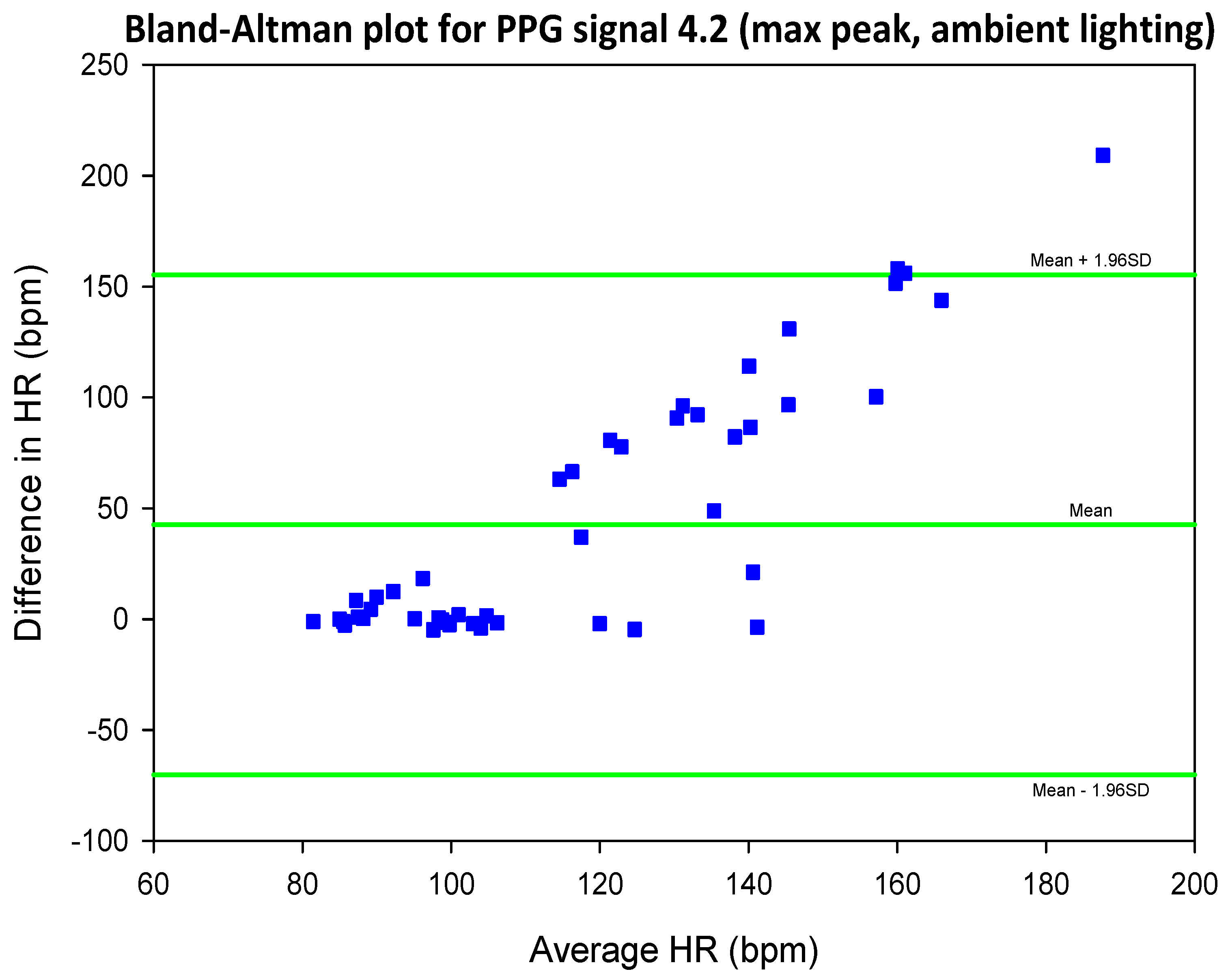
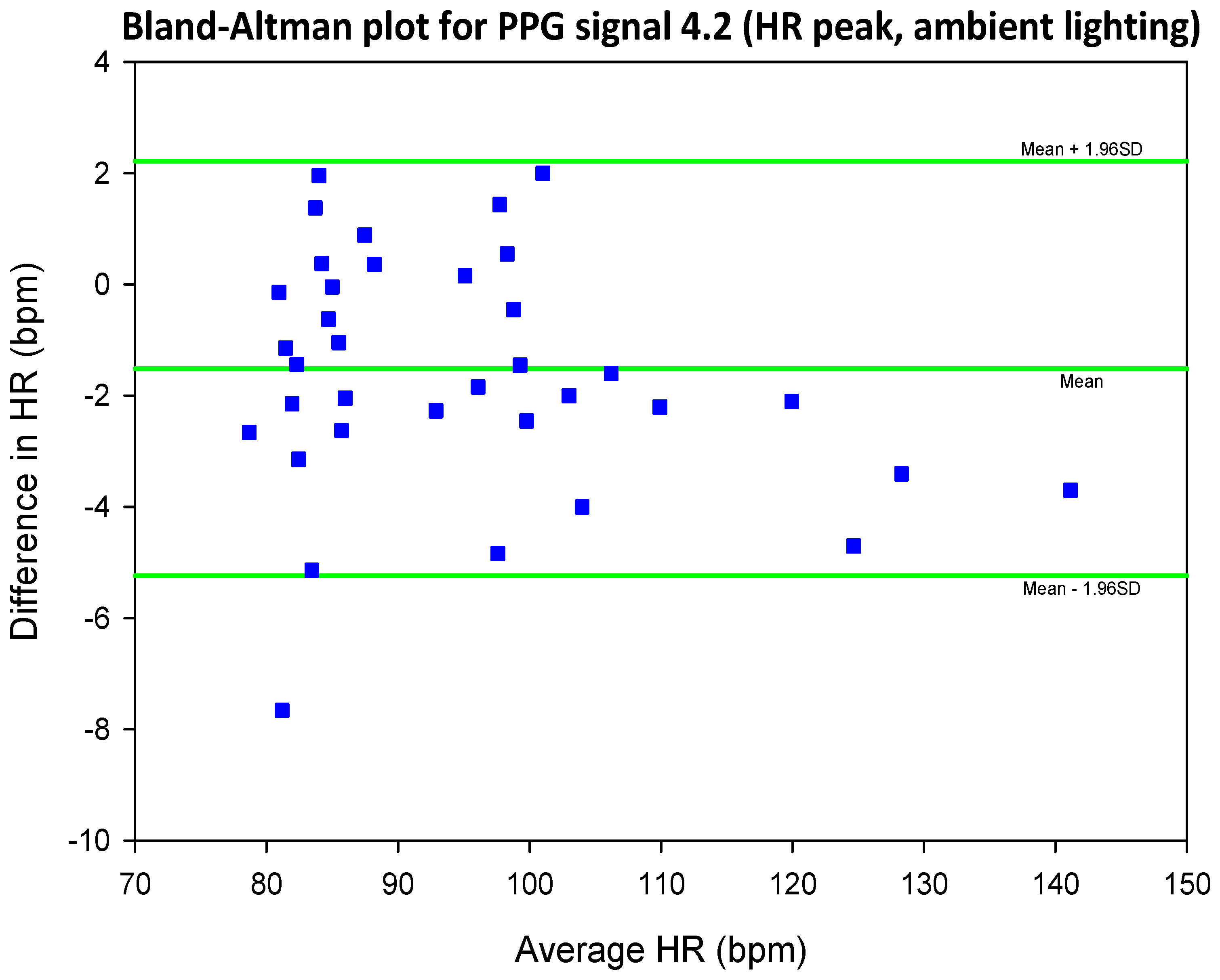
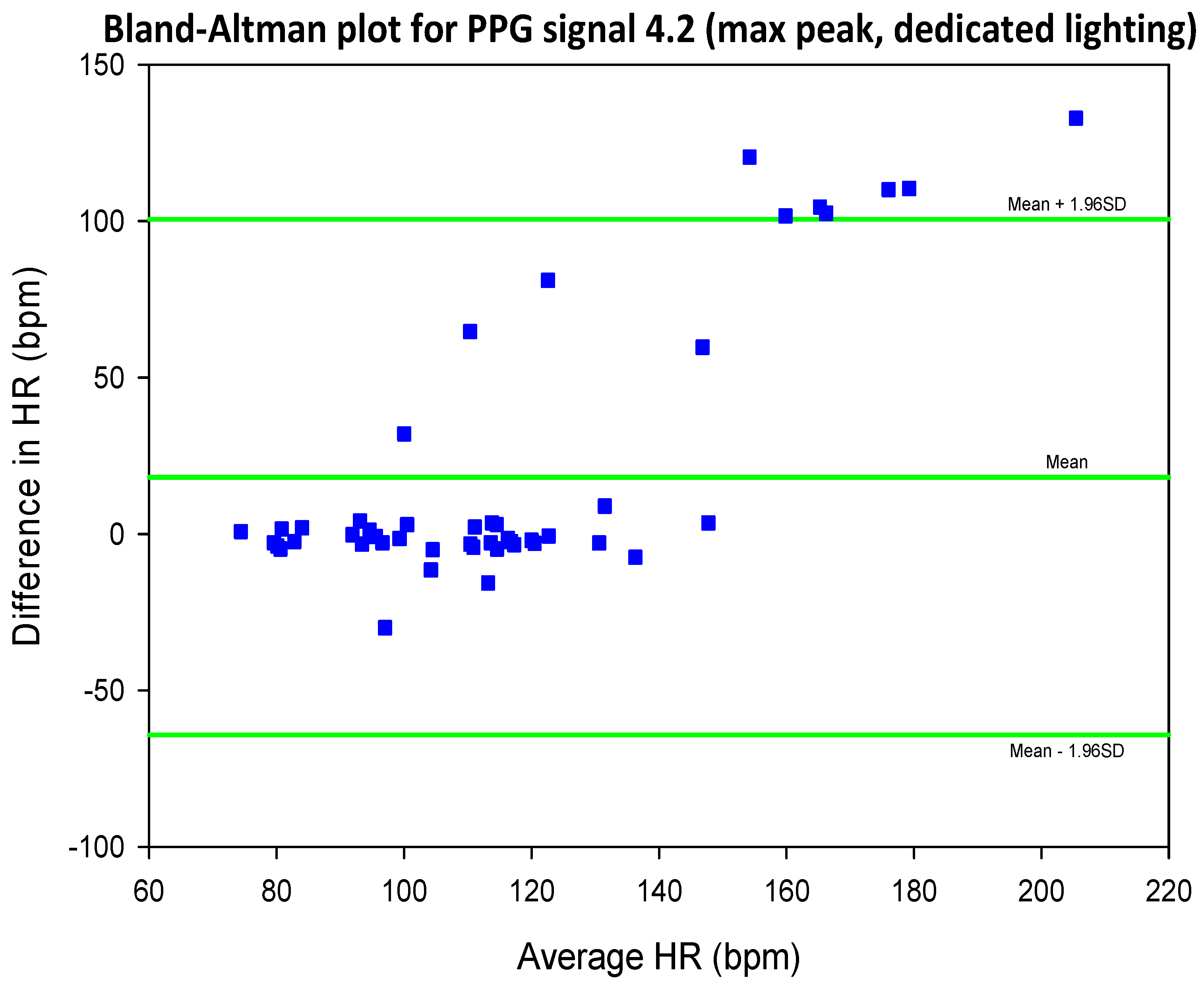
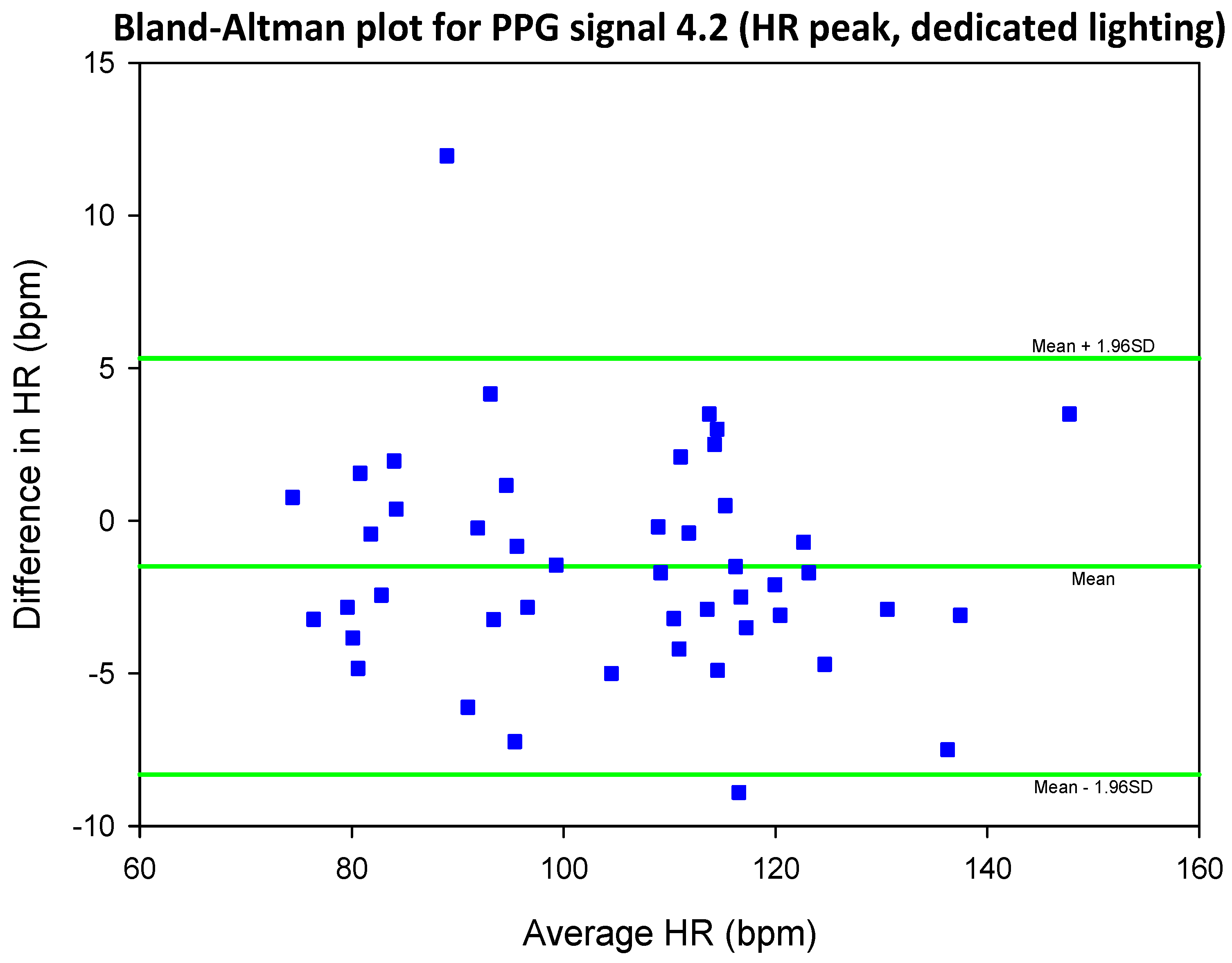
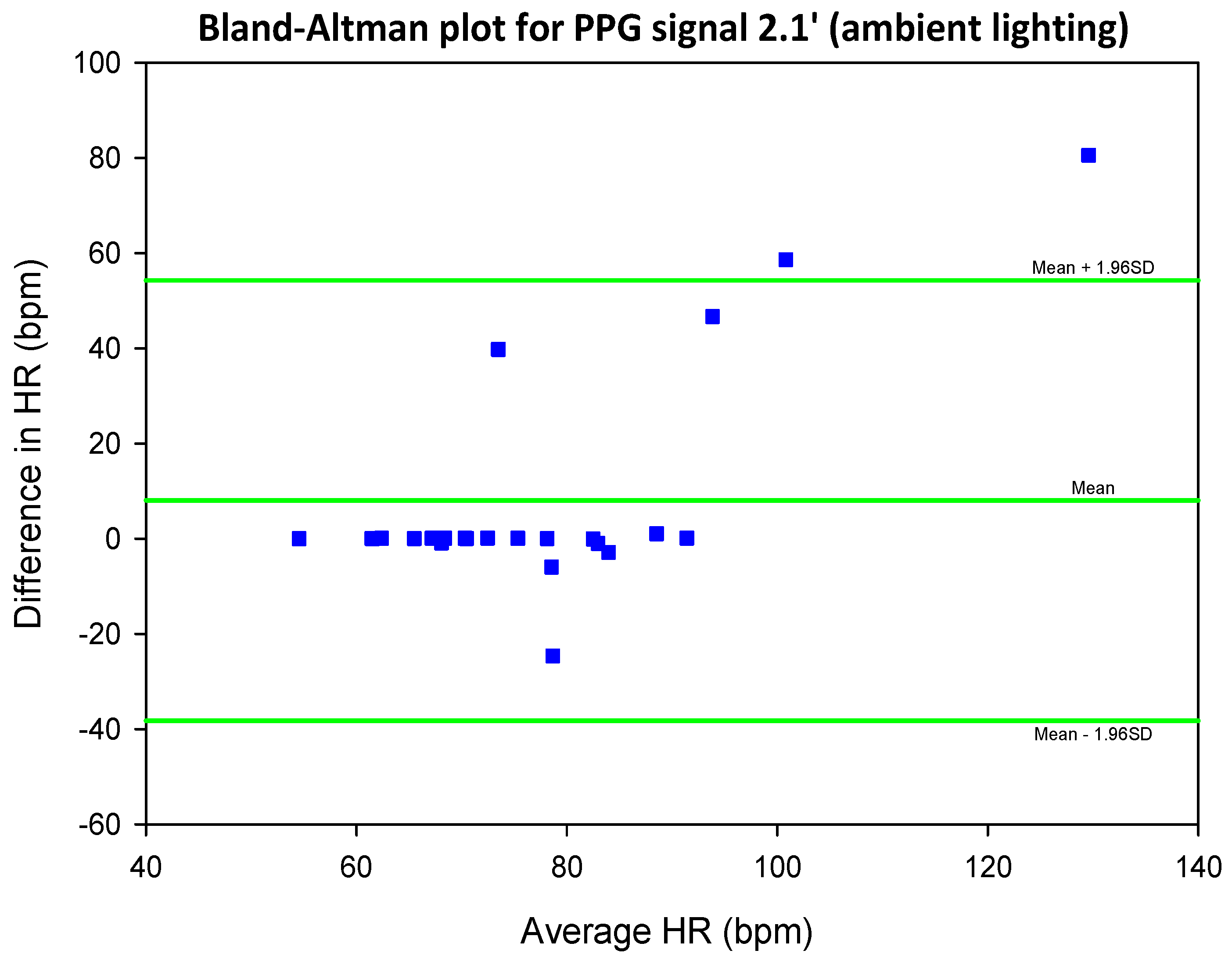
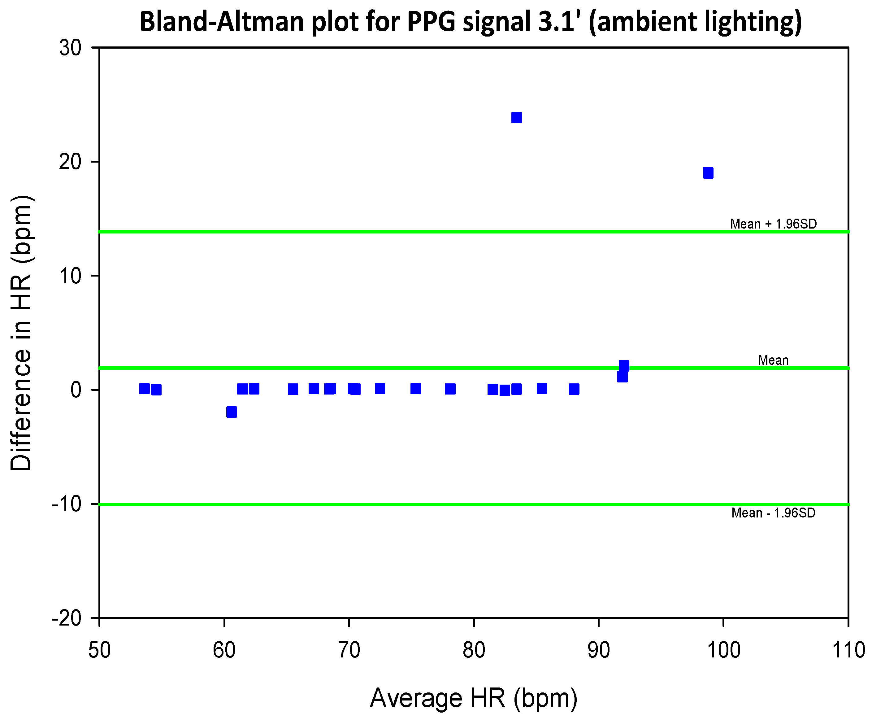
As a visual representation of agreement, Bland-Altman plots were prepared for signal 4.2 only. This signal displayed the lowest mean error and highest SNR (under both ambient and dedicated lighting) and was deemed most indicative of the success of the implementation of HR estimation by rPPG. The Bland-Altman plot is a popular graphical method for comparing two measurement techniques (in this case, HR measurement by rPPG and ground truth reference). In this method, the differences of values obtained using the two techniques are plotted against the average of the two values. The Bland-Altman plot is typically displayed with two sets of horizontal lines – one line representing the mean of the differences or systematic bias and two more representing the limits of agreement, defined as the mean difference ± 1.96 standard deviations. If these limits do not exceed the maximum allowed difference between methods, the two methods are considered in agreement. Bland-Altman analysis has significant advantages over correlation analysis as it represents the degree of agreement between methods and reveals both systematic and random errors. Correlation analysis, while it evaluates the strength of relationships between variables, does not evaluate agreement.
For max peak HR estimates under ambient lighting (Figure 5.1), the Bland-Altman plot reveals that rPPG systematically overestimate the HR by an average of approximately 50 bpm and that the variance of HR estimates increases with HR (as indicated by the greater spread). The plot also displays a proportional bias, whereby the degree of agreement between the two HR measures degrades with increasing HR. For signal peak HR estimates under ambient lighting (Figure 5.2), the Bland-Altman plot reveals a small bias of approximately -2 bpm i.e., rPPG underestimates the heart rate by an average of 2 bpm. The variance does not seem dependent on the magnitude of the heart rate, though there seems to be a bias towards underestimation at higher HRs.
Figure 5. 1. Bland-Altman plot for HR determined from rPPG signal 4.2 using max peak estimates (ambient lighting).
Preprints 69042 g024
Figure 5. 2. Bland-Altman plot for HR determined from rPPG signal 4.2 using signal peak estimates (ambient lighting).
Preprints 69042 g025
The Bland-Altman plot for max peak HR estimates under dedicated lighting (Figure 5.3) also shows a systematic overestimation of the heart rate, though by a smaller amount (approximately 20 bpm) relative to the ambient lighting case. It also displays some degree of a proportional bias, with higher disagreement at higher HRs. The Bland-Altman plot for signal peak HR estimates under dedicated lighting (Figure 5.4) displays a small HR underestimation of about 1 bpm, no proportional bias, and a random distribution of points about the mean.
Figure 5. 3. Bland-Altman plot for HR determined from rPPG signal 4.2 using max peak estimates (dedicated lighting).
Preprints 69042 g026
Figure 5. 4. Bland-Altman plot for HR determined from rPPG signal 4.2 using signal peak estimates (dedicated lighting).
Preprints 69042 g027
Referring to Table 5.5, mean SNR for the self-captured videos under ambient lighting ranged from 0.08 to 0.16. SNR improved significantly under dedicated lighting for each of the eight (8) rPPG signals (Table 5.6), with a minimum increase of 33% (for signal 1.2) and a maximum increase of 70% (for signal 2.1).
Table 5. 5. Mean SNR of rPPG signals (ambient lighting).
SIG1 SIG2 SIG3 SIG4
FFT Welch FFT Welch FFT Welch FFT Welch
Mean SNR 0.08 0.09 0.09 0.11 0.08 0.09 0.14 0.16
Table 5. 6. Mean SNR of rPPG signals (dedicated lighting).
SIG1 SIG2 SIG3 SIG4
FFT Welch FFT Welch FFT Welch FFT Welch
Mean SNR 0.12 0.12 0.16 0.16 0.12 0.13 0.22 0.23
As a supplement to the evaluation of agreement, Pearson correlation analysis was performed to evaluate the systematic relationship between rPPG HR estimates and reference values. In correlation analysis, the correlation coefficient (r) quantifies the linear relationship between two variables while its corresponding p-value determines whether the correlation is statistically significant. The correlation coefficient has a value ranging from +1 to –1, with +1 indicating perfect positive correlation, 0 indicating no correlation, and –1 indicating perfect negative correlation. The threshold value for p is the standard p = 0.05, meaning that only p-values less than 0.05 indicate statistical significance.
Max peak HR estimates under ambient lighting (Figure 5.7) all show weak negative correlation with ground truth HR, with only two statistically significant r values (r = – 0.28 and a max r = – 0.35 for signals 3.1 and 3.2, respectively). Correlation coefficients significantly increased for signal peak estimates (Table 5.8), showing strong positive correlations with all r = 0.99 and all p = 0.00 (indicating statistical significance in all cases).
Table 5. 7. Correlation coefficients (r) and p-values for est. HR vs ref. HR (max peak, ambient lighting).
SIG1 SIG2 SIG3 SIG4
FFT Welch FFT Welch FFT Welch FFT Welch
r -0.15 -0.03 -0.09 -0.06 -0.28 -0.35 -0.22 -0.13
p 0.29 0.84 0.56 0.68 0.05 0.01 0.13 0.35
Table 5. 8. Correlation coefficients (r) and p-values for est. HR vs ref. HR (signal peak, ambient lighting).
SIG1 SIG2 SIG3 SIG4
FFT Welch FFT Welch FFT Welch FFT Welch
r 0.99 0.99 0.99 0.99 0.99 0.99 0.99 0.99
p 0.00 0.00 0.00 0.00 0.00 0.00 0.00 0.00
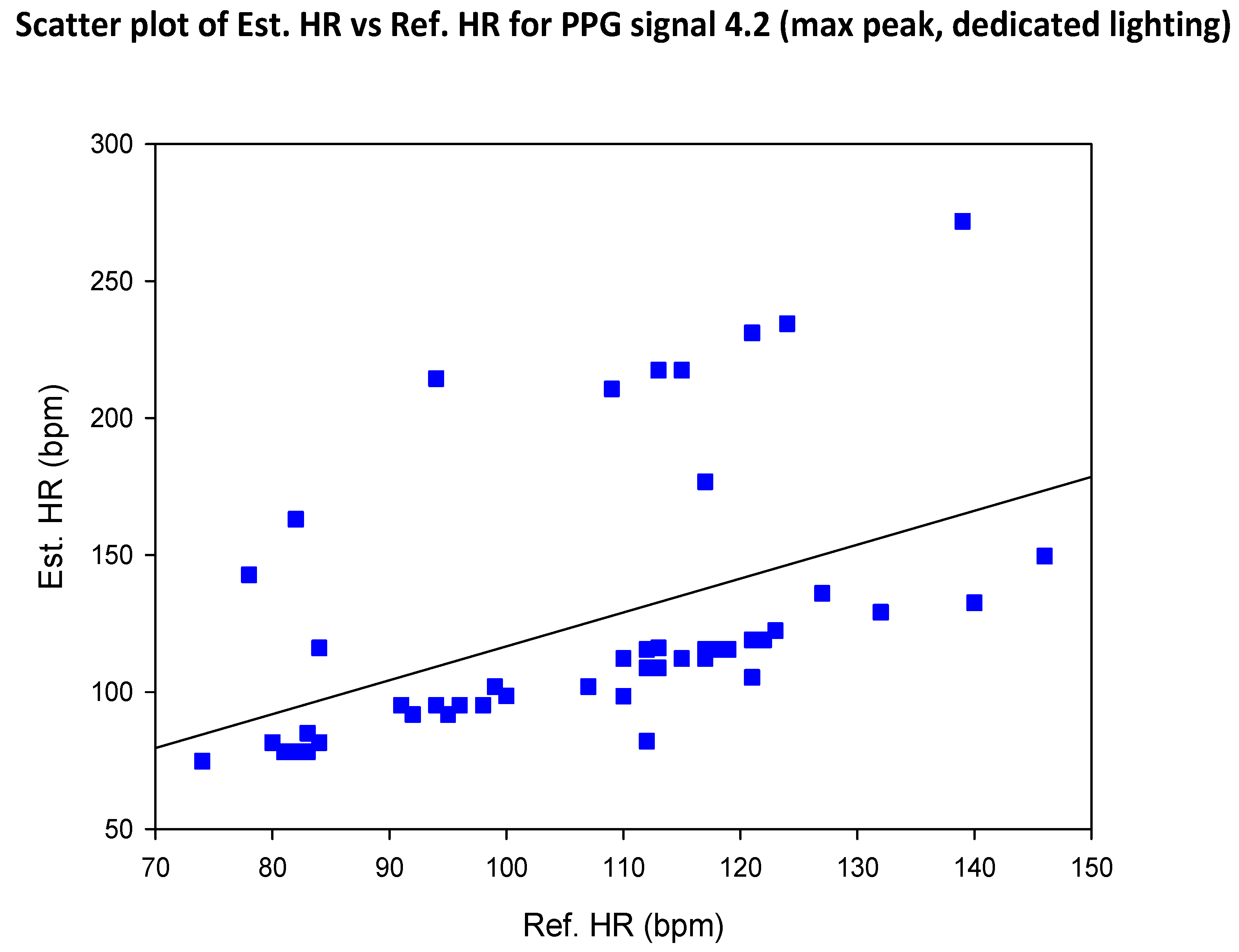
Max peak HR estimates under dedicated lighting (Table 5.9) all show positive correlation with ground truth HR, with two signals (4.1 and 4.2) showing statistical significance (r = 0.36 and r = 0.47, respectively). As in the case for ambient lighting, correlation coefficients significantly increased for signal peak estimates (Table 5.10), showing strong positive correlations with all r = 0.98 or 0.99 and all p = 0.00.
Table 5. 9. Correlation coefficients (r) and p-values for est. HR vs ref. HR (max peak, dedicated lighting).
SIG1 SIG2 SIG3 SIG4
FFT Welch FFT Welch FFT Welch FFT Welch
r 0.03 0.09 0.08 0.20 0.18 0.03 0.36 0.47
p 0.82 0.56 0.59 0.16 0.22 0.84 0.01 0.00
Table 5. 10. Correlation coefficients (r) and p values for est. HR vs ref. HR (signal peak, dedicated lighting).
SIG1 SIG2 SIG3 SIG4
FFT Welch FFT Welch FFT Welch FFT Welch
r 0.99 0.98 0.99 0.98 0.99 0.99 0.99 0.98
p 0.00 0.00 0.00 0.00 0.00 0.00 0.00 0.00
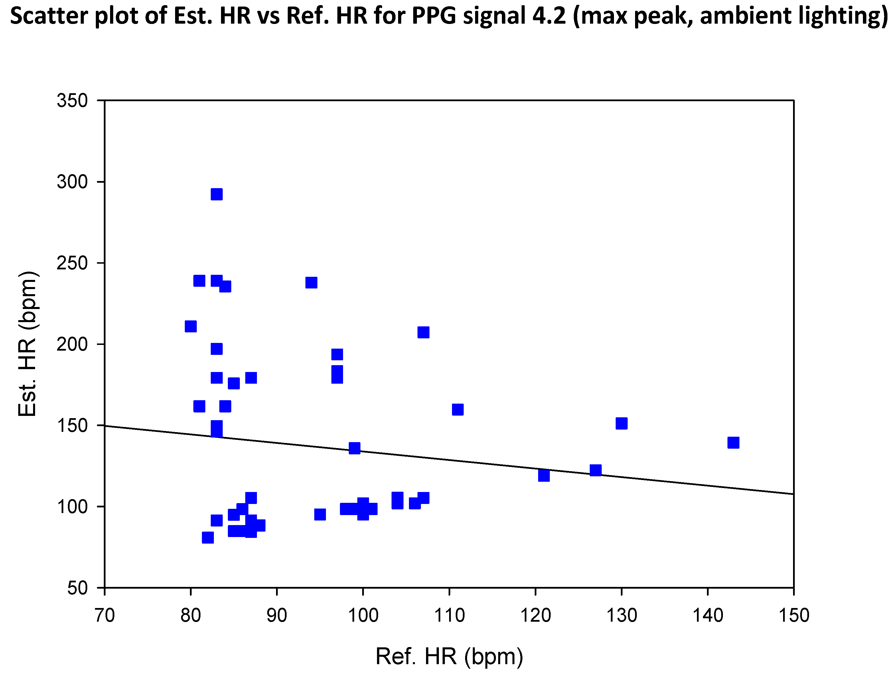
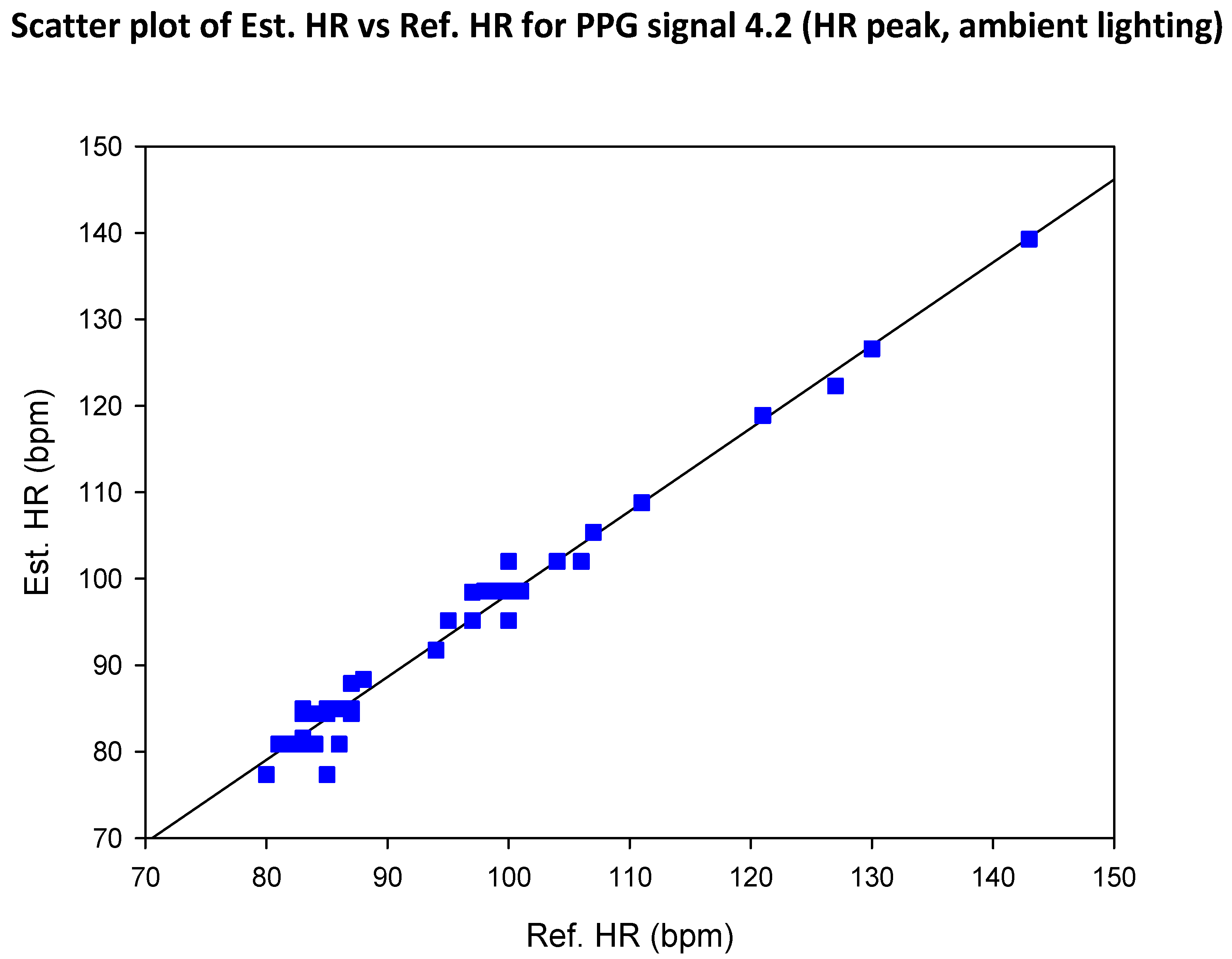
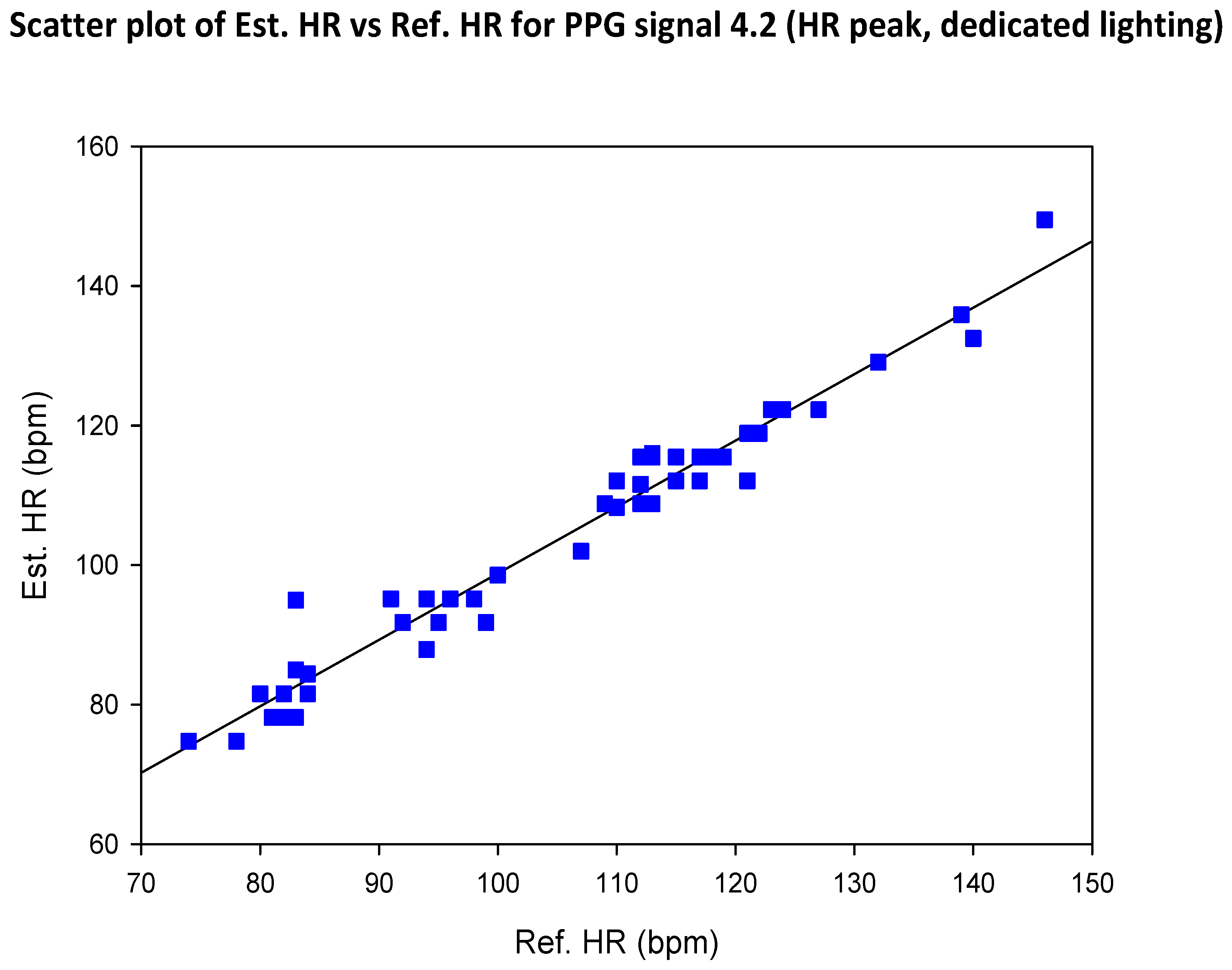
Correlation (scatter) plots were produced for signal 4.2. The plot for max peak estimates of HR under ambient lighting (Figure 5.5) shows a negative slop (negative correlation) and a general decrease in the variance of the estimated HR with increasing reference HR. This correlation is, however, weak (r = -0.13) and not statistically significant (p = 0.35). For the corresponding signal peak estimates (Figure 5.6), the correlation between HR estimates and reference values is visibly strong and positive (r = 0.99, p = 0.00).
Figure 5. 5. Scatter plot of est. HR versus ref. HR for rPPG signal 4.2 (max peak, ambient lighting).
Preprints 69042 g028
Figure 5. 6. Scatter plot of est. HR versus ref. HR for rPPG signal 4.2 (signal, ambient lighting).
Preprints 69042 g029
For max peak estimates of HR under dedicated lighting (Figure 5.7), the correlation between estimates and reference values is positive, moderate (r = 0.47) and statistically significant (p = 0.00). The distribution of points also indicates significant variance in the estimated HR. However, unlike the ambient lighting case, this variance is fairly constant with increasing reference HR. For the corresponding signal peak estimates (Figure 5.8), as in the ambient lighting case, the correlation is strong and positive (r = 0.98, p = 0.00).
Figure 5. 7. Scatter plot of est. HR versus ref. HR for rPPG signal 4.2 (max peak, dedicated lighting).
Preprints 69042 g030
Figure 5. 8. Scatter plot of est. HR versus ref. HR for rPPG signal 4.2 (signal peak, dedicated lighting).
Preprints 69042 g031
A correlation analysis was also performed for error of HR estimates versus SNR to assess the impact of SNR on error. For the case of ambient lighting (Table 5.11), correlation coefficients ranged from -0.47 to -0.69 (moderate to strong correlation), with all p = 0.00. For the case of dedicated lighting (Table 5.12), the correlation coefficients ranged from -0.43 to -0.52 (moderate correlation), with all p = 0.00.
Table 5. 11. Correlation coefficients (r) and p-values for error versus SNR (ambient lighting).
SIG1 SIG2 SIG3 SIG4
FFT Welch FFT Welch FFT Welch FFT Welch
r -0.50 -0.55 -0.47 -0.56 -0.54 -0.60 -0.63 -0.69
p 0.00 0.00 0.00 0.00 0.00 0.00 0.00 0.00
Table 5. 12. Correlation coefficients (r) and p-values for error versus SNR (dedicated lighting).
SIG1 SIG2 SIG3 SIG4
FFT Welch FFT Welch FFT Welch FFT Welch
r -0.45 -0.43 -0.44 -0.46 -0.48 -0.43 -0.45 -0.52
p 0.00 0.00 0.00 0.00 0.00 0.00 0.00 0.00
Correlation plots of error versus SNR were produced for signal 4.2. As indicated, correlations are negative for both the ambient lighting and dedicated lighting case (Figures 5.9 and 5.10), with the point distributions showing significant variance in both cases.
Figure 5. 9. Scatter plot of error versus SNR for rPPG signal 4.2 (ambient lighting).
Preprints 69042 g032
Figure 5. 10. Scatter plot of error versus SNR for rPPG signal 4.2 (dedicated lighting).
Preprints 69042 g033

5.2. COHFACE Database Videos

Mean error (and RMSE) of HR estimates for COHFACE videos were far superior to that of self-captured videos. Referring to Tables 5.13 and 5.14, mean error of HR estimates ranged from 3% to 15% under ambient lighting and 0% to 9% under dedicated lighting. Interestingly, the worst case mean error for the COHFACE videos (15%, ambient lighting) significantly outperforms the best case mean error for the self-captured videos (22%, dedicated lighting).
Table 5. 13. Mean error and RMSE of HR estimates (ambient lighting).
SIG1′ SIG2′ SIG3′ SIG4′
FFT Welch FFT Welch FFT Welch FFT Welch
Mean Error 0.08 0.15 0.15 0.12 0.03 0.09 0.08 0.10
RMSE 14.88 24.37 24.46 18.14 6.27 14.85 16.27 16.32
Table 5. 14. Mean error and RMSE of HR estimates (dedicated lighting).
SIG1′ SIG2′ SIG3′ SIG4′
FFT Welch FFT Welch FFT Welch FFT Welch
Mean Error 0.01 0.02 0.02 0.09 0.01 0.02 0.00 0.01
RMSE 1.71 3.12 5.41 13.66 2.19 1.73 0.32 1.05
The high level of accuracy obtained for COHFACE videos is reflected in Bland-Altman plots drawn only for the worst performing (signal 2.1′) and best performing FFT signals (signal 3.1′) (to provide a visual display of the range of accuracy). In this context, determination of the best and worst performing signal was based on mean error of HR estimates under ambient lighting. All Bland-Altman plots (Figures 5.11, 5.12, 5.13 and 5.14) display a small or negligible bias in mean differences (with a maximum of approximately +10 bpm for signal 2.1′, ambient lighting) with no indication of systematic error. Perhaps a worthy observation revealed by the Bland-Altman plots is that significant difference between estimated and reference HR tends to involve an overestimation (as opposed to an underestimation), possibly indicating the observed tendency of strong noisy peaks in the higher frequency portion of the spectrum.
Figure 5. 11. Bland-Altman plot for HR determined from sig 2.1′ (ambient lighting).
Preprints 69042 g034
Figure 5. 12. Bland-Altman plot for HR determined from sig 3.1′ (ambient lighting).
Preprints 69042 g035
Figure 5. 13. Bland-Altman plot for HR determined from sig 2.1′ (dedicated lighting).
Preprints 69042 g036
Figure 5. 14. Bland-Altman plot for HR determined from sig 3.1′ (dedicated lighting).
Preprints 69042 g037
Mean SNR for COHFACE videos ranged from 0.26 to 0.36 under ambient lighting (Table 5.15) and 0.43 to 0.68 under dedicated lighting (Table 5.16). This represents marked improvement in mean SNR under dedicated lighting (for each of the 8 rPPG signals), with a minimum increase of 59% (for signal 2.2′) and a maximum increase of 104% (for signal 1.1′). A noteworthy observation (like that observed for mean error) is that the worst-case SNR for the COHFACE videos (0.26) is superior to the best-case SNR for the self-captured videos (0.23).
Table 5. 15. Mean SNR for rPPG signals (ambient lighting).
SIG1′ SIG2′ SIG3′ SIG4′
FFT Welch FFT Welch FFT Welch FFT Welch
Mean SNR 0.27 0.28 0.26 0.27 0.35 0.35 0.36 0.36
Table 5. 16. Mean SNR for rPPG signals (dedicated lighting).
SIG1′ SIG2′ SIG3′ SIG4′
FFT Welch FFT Welch FFT Welch FFT Welch
Mean SNR 0.55 0.55 0.43 0.43 0.68 0.68 0.63 0.62
Correlation coefficients (r) and corresponding p-values for estimated HR versus reference HR were calculated for the 8 rPPG signals under ambient and dedicated lighting, taken separately, and together. Table 5.17 shows correlation coefficients ranging from a weak 0.26 (p = 0.22, signal 2.2′) to a strong 0.90 (p = 0.00, signal 3.1′) for ambient lighting, with only three of the eight r values statistically significant. Referring to Table 5.18, correlation coefficients ranged from 0.55 (signal 2.2′) to 1.00 (signal 4.1′) (all but one r value < 0.9) for dedicated lighting, with all p-values indicating statistical significance (all except one equal to 0.00). For rPPG signals considered together (ambient + dedicated) (Table 5.19), correlation coefficients ranged from a weak 0.39 (signal 2.2′) to a very strong 0.93 (signal 3.1′), with the coefficients generally bearing a value between that obtained for their equivalents under ambient and dedicated lighting. The p-values exactly reproduced the results obtained for dedicated lighting.
Table 5. 17. Correlation coefficients (r) and p-values for est. HR vs ref. HR (ambient lighting).
SIG1′ SIG2′ SIG3′ SIG4′
FFT Welch FFT Welch FFT Welch FFT Welch
r 0.39 0.69 0.39 0.26 0.90 0.53 0.39 0.33
p 0.06 0.00 0.06 0.22 0.00 0.01 0.06 0.12
Table 5. 18. Correlation coefficients (r) and p-values for est. HR vs ref. HR (dedicated lighting).
SIG1′ SIG2′ SIG3′ SIG4′
FFT Welch FFT Welch FFT Welch FFT Welch
r 0.99 0.96 0.93 0.55 0.98 0.99 1.00 1.00
p 0.00 0.00 0.00 0.01 0.00 0.00 0.00 0.00
Table 5. 19. Correlation coefficients (r) and p-values for est. HR vs ref. HR (all videos).
SIG1′ SIG2′ SIG3′ SIG4′
FFT Welch FFT Welch FFT Welch FFT Welch
r 0.64 0.68 0.56 0.39 0.93 0.70 0.62 0.59
p 0.00 0.00 0.00 0.01 0.00 0.00 0.00 0.00
Correlation (scatter) plots were also prepared for the worst and best signals (2.1′ and 3.1′, respectively) under ambient and dedicated lighting (Figures 5.15, 5.16, 5.17 and 5.18). All plots display strong positive correlation, with very few (≤ 2) significant deviations from the line of best fit (except in the case of signal 2.1′ under ambient lighting, where there are five (5) significant deviations).
Figure 5. 15. Scatter plot of est. HR versus ref. HR for sig 2.1′ (ambient lighting).
Preprints 69042 g038
Figure 5. 16. Scatter plot of est. HR versus ref. HR for sig 3.1′ (ambient lighting).
Preprints 69042 g039
Figure 5. 17. Scatter plot of est. HR versus ref. HR for sig 2.1′ (dedicated lighting).
Preprints 69042 g040
Figure 5. 18. Scatter plot of est. HR versus ref. HR for sig 2.1′ (dedicated lighting).
Preprints 69042 g041

6. Discussion

This chapter discusses the results of the preceding chapter in relation to the research objectives set forth in Chapter 1. For each objective, the results for the self-captured videos will be discussed first, followed by that for the COHFACE videos, which will make comparative references where relevant.

6.1. Implement an Algorithmic Framework for HR Estimation by Video-Based Reflectance Photoplethysmography
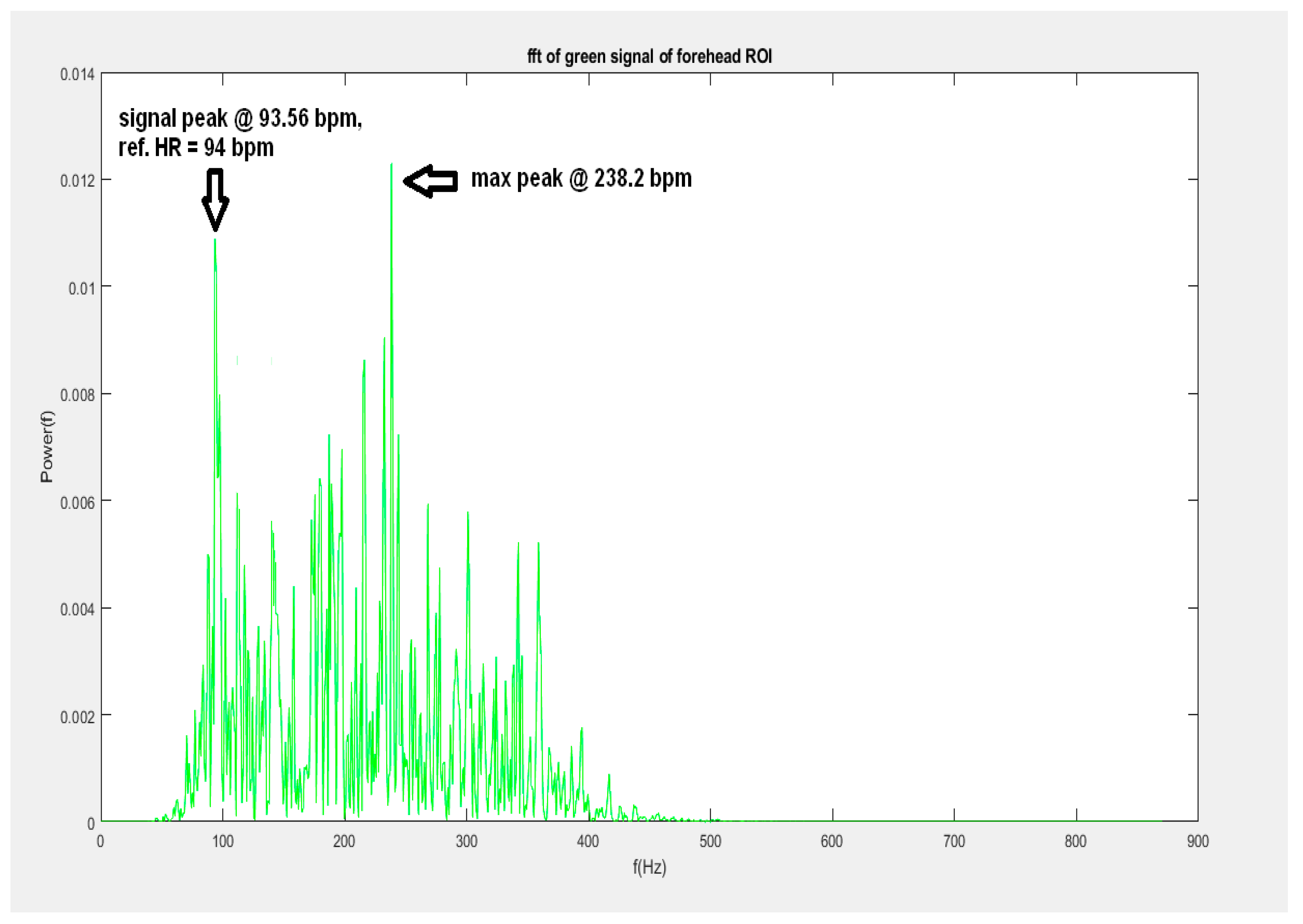
The primary objective of this thesis was to set up an algorithmic framework for the estimation of HR by the analysis of rPPG signals extracted from video. Accordingly, an immediate concern is whether the framework is set up correctly. Such validity may be evaluated through the level of agreement between rPPG HR estimates and reference (ground truth) values. Agreement was assessed using two statistical measures – mean error and root-mean-square error (RSME)1 – as well as Bland-Altman plots. Correlation (scatter) plots, while not representing agreement, were also used to assess the systematic relationship between estimated and reference values. Another performance metric used in this investigation is the signal-to-noise ratio (SNR) – a primary measure of signal quality significantly correlated with the error in HR estimates.
SNR for rPPG signals extracted from the self-captured videos was generally low. This is primarily ascribed to the dark skin tone of the subject as it is known that rPPG SNR is particularly low for dark skin. This presented a significant drawback to the evaluation of agreement between rPPG HR estimates and reference values. In many cases, low SNR resulted in a peak of maximum amplitude at a frequency other than the HR (with the peak representing the HR still dominant). Figure 6.1 illustrates a typical instance of a noisy peak predominating the peak representing the HR (termed interchangeably signal peak or heart rate peak in this thesis). As discussed in Materials and Methods, this limitation was addressed by using two criteria for assessing agreement:
considering only maximum peaks in the HR estimation and
considering signal peaks, which may or may not be maximum peaks.
Figure 6. 1. Representative example of signal peak in relation to maximum peak.
Preprints 69042 g042
Tables 5.1 and 5.3 show mean error (based on max peak HR estimates) ranging from 50% to 119% for rPPG signals extracted under ambient lighting and 22% to 61% for signals extracted under dedicated lighting. The improvement in accuracy under dedicated lighting is imputed to increased SNR (mean SNR ranged from 0.08 to 0.16 and 0.12 to 0.23 under ambient and dedicated lighting, respectively). This immediately gives a sense of the impact of SNR on mean error, which drastically improved for signal peak estimates of HR (2% for every signal under ambient lighting and 3% for every signal under dedicated lighting).
In this investigation, there is a possibility that good accuracy values arose from systematic error rather than actual agreement between estimated and reference HR. For example, if a spurious peak consistently exists in the region of say 80 bpm and the investigated range of HR is, say, 78 – 82 bpm, then highly accurate HR estimates could be seemingly obtained even if the rPPG signal contains no HR information. To address this possibility a large range of HRs were obtained for self-captured videos (both resting and post-exercise) and a correlation analysis was performed between estimated and reference values. Max peak HR estimates under ambient lighting all displayed weak negative correlation with ground truth HR, with only two statistically significant correlations. This unexpectedly negative correlation may be explained in terms of the randomizing effect of noise on max peak HR estimates. Max peak HR estimates under dedicated lighting all displayed positive correlation with ground truth HR, with two signals (4.1 and 4.2) showing statistical significance. With the correlations bearing the expected sign (notwithstanding that only two are statistically significant), this may be deemed an improvement over ambient lighting case. This improvement is ascribed to a reduction in the effect of the randomization on the HR estimates due to improved SNR under dedicated lighting. Correlation coefficients for HR estimates versus ground truth significantly increased for signal peak HR estimates, showing strong positive and statistically significant correlations under ambient and dedicated lighting. This correlation analysis supported the view that, despite the interference caused by low SNR, HR estimates latently tracked ground truth values and can be considered legitimate.
To further support the proposition that poor accuracy stemmed from low SNR, a correlation analysis was performed for the error in HR estimates versus SNR for each of the 8 rPPG signals. For the case of ambient lighting, correlation coefficients ranged from -0.47 to -0.69 (moderate to strong correlation). For the case of dedicated lighting, coefficients ranged from -0.43 to -0.52, reflecting moderate correlation in the expected direction. Though correlations are too weak to ascribe all inaccuracy to low SNR, it does indicate that low SNR significantly accounts for loss of accuracy.
For the COHFACE videos, a resolution of the problems related to generally low mean SNR was obviated as the COHFACE rPPGs displayed comparatively high mean SNR for both the dedicated and ambient lighting case. As such, there was no need for a separate evaluation of measures of agreement based on signal peaks; in (virtually) every case, the signal peak was the maximum peak. The high SNR (and correspondingly low mean error and RMSE) also nullified the relevance of an assessment of the correlation between error and SNR (performed for the self-captured videos).
Mean error of HR estimates for COHFACE videos ranged from 3% to 15% under ambient lighting and 0% to 9% under dedicated lighting. Importantly, the worst case mean error for the COHFACE videos (15%, ambient lighting) significantly outperformed the best case mean error for the self-captured videos (22%, dedicated lighting). This highlights the impact of SNR on accuracy performance.
Correlation coefficients (r) and p-values for estimated HR versus reference HR were calculated for the eight (8) rPPG signals under ambient and dedicated lighting (Tables 5.17 and 5.18). Correlation coefficients ranged from a weak 0.26 to a strong 0.90 for ambient lighting, with p-values indicating only three (3) statistically significant correlations. These unexpectedly poor correlations, despite generally high corresponding mean accuracies, reflect the sensitivity of the correlation measure to outliers. The strength and significance of correlations, however, showed marked improvement under dedicated lighting, with coefficients ranging from 0.55 to 1.00 (all but one r value < 0.9), with all p-values negligible. This could easily be explained in terms of the increase in accuracy (and reduced number of outliers) associated with the improvement in SNR afforded by dedicated lighting.
Mean SNR for rPPG signals extracted from COHFACE videos ranged from 0.26 to 0.36 under ambient lighting (Table 5.15) and 0.43 to 0.68 under dedicated lighting (Table 5.16). A significant observation (like that observed for mean error) is that the worst-case SNR for the COHFACE videos is superior to the best-case SNR for the self-captured videos (0.23), giving an indication of the strength of the impact of skin tone on SNR performance.

6.2. Investigate the Effect of Presence/Absence of Dedicated Lighting on the SNR of rPPG Signals

Apart from setting up a correct algorithmic framework for rPPG extraction and analysis, another major point of investigation was the effect of the presence/absence of dedicated lighting on the mean SNR of rPPG signals.
For the self-captured videos (Tables 5.5 and 5.6), mean SNR improved significantly under dedicated lighting (relative to ambient lighting) for each of the eight (8) rPPG signals, with a minimum increase of 33% in the case of signal 1.2 and a maximum increase of 70% in the case of signal 2.1. Mean SNR also improved significantly under dedicated lighting (Table 5.15 and 5.16) for the signals extracted from the COHFACE videos, with a minimum increase of 59% (for signal 2.2′) and a maximum increase of 104% (for signal 1.1′). This increase in SNR is consistent with theoretical expectation as the greater the light intensity, the greater the reflected component in relation to noisy fluctuations arising from motion and/or background illumination.
It is also important to note that mean SNR for the rPPG signals extracted from the COHFACE videos, even under ambient lighting, surpassed that for the self-captured videos under dedicated lighting. This is indicative of the extent to which dark skin tone (self-captured videos) can degrade SNR performance.

6.3. Investigate the Effect of Choice/Size of Region of Interest (ROI) on the SNR of rPPG Signals

Another objective of this thesis was to investigate the effect of the choice/size of the ROI for rPPG signal extraction on the SNR of the signals. Three ROIs were investigated. The description of each ROI – termed A, B and C – is provided in Table 3.1. ROI B was expected to yield a higher SNR than ROI A since their only significant difference is that ROI B is 50% larger than ROI A (they are both centred on the forehead and contain only skin pixels). All things being equal, the SNR of two images scales as the square root of the number of pixels. It was also hypothesized that ROI C would be inferior in SNR relative to ROI B (and possibly also ROI A), notwithstanding its superior size, since it contains a large percentage of non-skin pixels and non-rigid structures (such as the eyes and mouth) which contribute to signal noise.
For the self-captured videos under ambient lighting (Table 5.5), ROI A yielded a mean SNR of 0.08 for the FFT signal and 0.09 for the Welch periodogram (Welch) signal. The corresponding values for ROI B were also 0.08 and 0.09 while that for ROI C were 0.14 and 0.16. While the SNRs for ROI A and B are equivalent, that for ROI C (invalidating hypothesis) is approximately twice as large (relative to ROI A or B). The difference may be explained in terms of the large number of skin pixels contained in ROI C coupled with minimal motion of the eyes and mouth by the subject. It is not clear why ROI B did not yield a higher mean SNR relative to ROI A. A possible explanation is that the size difference in the ROIs was not significant enough to produce a statistically significant difference in the SNR.
For the self-captured videos under dedicated lighting (Table 5.6), ROI A yielded a mean SNR of 0.12 for both the FFT and Welch signal. ROI B performed comparably, yielding a mean SNR of 0.12 for the FFT and 0.130 for the Welch. Just as in the case of ambient lighting, ROI C displayed a significantly higher mean SNR at 0.22 for the FFT and 0.23 for the Welch.
For the COHFACE videos under ambient lighting (Table 5.15), the mean SNRs for ROIs A, B and C were 0.27, 0.35 and 0.36 (respectively) for the FFT, and 0.28, 0.35 and 0.36 for the Welch. Under dedicated lighting (Table 5.16), corresponding values were 0.55, 0.68 and 0.63 for the FFT and 0.55, 0.68 and 0.62 for the Welch. ROIs B and C may be described as comparable in SNR performance (with C slightly superior to B under ambient lighting, and B superior to C under dedicated lighting) and superior to ROI A. The commonality between the results for the self-captured videos and that for the COHFACE videos is that they both indicate superiority of ROI C. However, while comparability exists between ROIs A and B for the self-captured videos, it exists between ROIs B and C for the COHFACE videos (with ROI B significantly outperforming ROI A). This difference may be explained by the hypothesis that the SNR difference (due to size difference) between ROIs B and A becomes more significant for all signals at higher SNR (as is the case for the COHFACE videos with a mean SNR under ambient lighting greater than that of the self-captured videos under dedicated lighting). As with the self-captured videos, the high SNR of ROI C is believed to be a direct consequence of its superior size. Again, minimal motion of the eyes and mouth may explain why noise did not override the size advantage and degrade the SNR of ROI C.
This analysis reveals ROI C as a simple high SNR ROI, perhaps useful in the case of optimizing SNR for dark skin and/or low lighting conditions. However, the SNR performance of ROI C may not hold under significant motion, and for this reason ROI B may prove a more robust option (given its comparability to ROI C in SNR performance and status as a forehead ROI containing only skin pixels and no non-rigid structures). An even better ROI may be designed using a skin mask with the eyes and mouth regions removed (to maximize the number of useful pixels and minimize the motion-induced noise).

6.4. Compare the SNR of Green rPPG Signals with That of rPPG Signals Based on Luminance

Given that reflectance photoplethysmography is based on variations in the intensity of light reflected from the skin, an evaluation of the SNR of a luminance-based rPPG signal relative to that of a color-based signal seemed appropriate. For the RGB color space, both hue and light intensity information are coded in the same channel. However, for color spaces containing luminance components (such as YCbCr and HSV), light intensity (luminance) information is coded independently of hue information. In this investigation, the YCbCr color space was used to provide the luminance component Y.
Referring to Tables 5.5 and 5.6, for the self-captured videos, mean SNR for the luminance signal (signal 2) under ambient lighting is 0.09 for the FFT and 0.11 for the Welch periodogram compared to 0.08 and 0.09 for its green counterpart (signal 1). Under dedicated lighting, the SNR for the luminance signal is 0.16 for both the FFT and Welch compared to 0.12 for the green signal (both FFT and Welch). This indicates that the luminance signal slightly outperforms its green counterpart in terms of SNR. A secondary comparison of mean error (based on maximum peaks) shows that the luminance signal also outperforms its green equivalent with a mean error of 75% (FFT) and 63% (Welch) for ambient lighting and 39% (FFT and Welch) under dedicated lighting, compared to the green signal’s 113% and 95%, and 57% and 48%, respectively.
For the COHFACE videos, Tables 5.15 and 5.16 show that the mean SNR for the luminance signal (signal 2′) under ambient lighting is 0.26 (FFT) and 0.27 (Welch) compared to 0.27 (FFT) and 0.28 (Welch) for its green equivalent (signal 1′). Under dedicated lighting, the mean SNRs are 0.43 for the luminance signal (both FFT and Welch) and 0.55 for its green counterpart (both FFT and Welch). These results indicate that the green signal outperforms the luminance signal in SNR (though only slightly in the case of ambient lighting) and inverts the finding for the self-captured videos. However, since the mean parameters for the COHFACE rPPG signals were based on a larger sample size (12 subjects), the superiority of the green signal over the luminance signal is a safer conclusion. Still, the contradictory results may warrant an investigation into the SNR performance of green versus luminance signals for dark-skinned subjects compared to fair-skinned subjects. It may very well be that the luminance signal is superior in SNR for dark tones but inferior for fair tones. A secondary consideration of mean error for the luminance and green signal reveals the green signal to be superior in every case except one (the case of the Welch signals under ambient lighting).

6.5. Investigate the Viability of the Summary Autocorrelation Function (SACF) for Improving the SNR of rPPG Signals

Summary autocorrelation is a technique conventionally used in speech processing for identifying fundamental frequencies. In this thesis, it was hypothesized that the technique could be used to improve the SNR of the rPPG signals. However, preliminary results for HR estimates using the SACF for spectral analysis did not bear any correlation with reference values. Assuming the technique can in fact accomplish the stated objective, the troubleshooting of the problems with the implementation was deemed too rudimentary to warrant a reporting of results. However, the theoretical soundness of the idea warrants further investigation. Accordingly, the technique is given consideration under further work.

6.6. Implement the HR Estimation Algorithm into a GUI

In keeping with objective 6 of this thesis, the HR estimation algorithm was implemented within a graphical user interface (GUI) to facilitate user-friendly interaction. The GUI was programmed using MATLAB GUIDE (GUI development environment) which provides tools for graphical design of user interfaces for custom applications. GUIDE automatically generates the MATLAB code for constructing the GUI, which can then be modified to program the behavior of the application.
There are two GUI components depending on the level of interaction desired by the user. The first GUI component (GUI1) is designed to facilitate a high level of user interaction with the data to provide more direct exposure to the analysis of signals in the frequency space. The second GUI component (GUI2), on the other hand, is structured to simply output HR estimates and matching ground truth values (in real time) for monitoring and/or recording, without any presentation of rPPG signals and analysis in the frequency space.
GUI1 contains a pushbutton at the top of the of GUI window for browsing and selecting a pre-recorded video (SELECT VIDEO) and an adjacent pushbutton for initiating video processing (labelled PROCESS VIDEO). After processing, the FFTs of signals 1 – 4 automatically appear in labelled panels. The Welch periodogram of these signals are also accessible by pressing the pushbutton labelled WELCH at the bottom of the GUI window. Return to FFT can be achieved by pressing the same button, which is automatically relabelled FFT. By identifying the frequency peaks of the FFTs and the Welch periodograms, users can estimate the HR associated with their input videos. A fuller explanation of the functionality of GUI1 will be provided in Appendix C where the GUI will serve as the interface for a laboratory experiment centred on HR estimation by video-based rPPG.
GUI2 is displayed in Figure 6.2. It contains a START pushbutton for synchronized initiation of three events:
  • live video capture and processing
  • a timer and,
  • a continuous display of the ground truth pulse oximeter signal
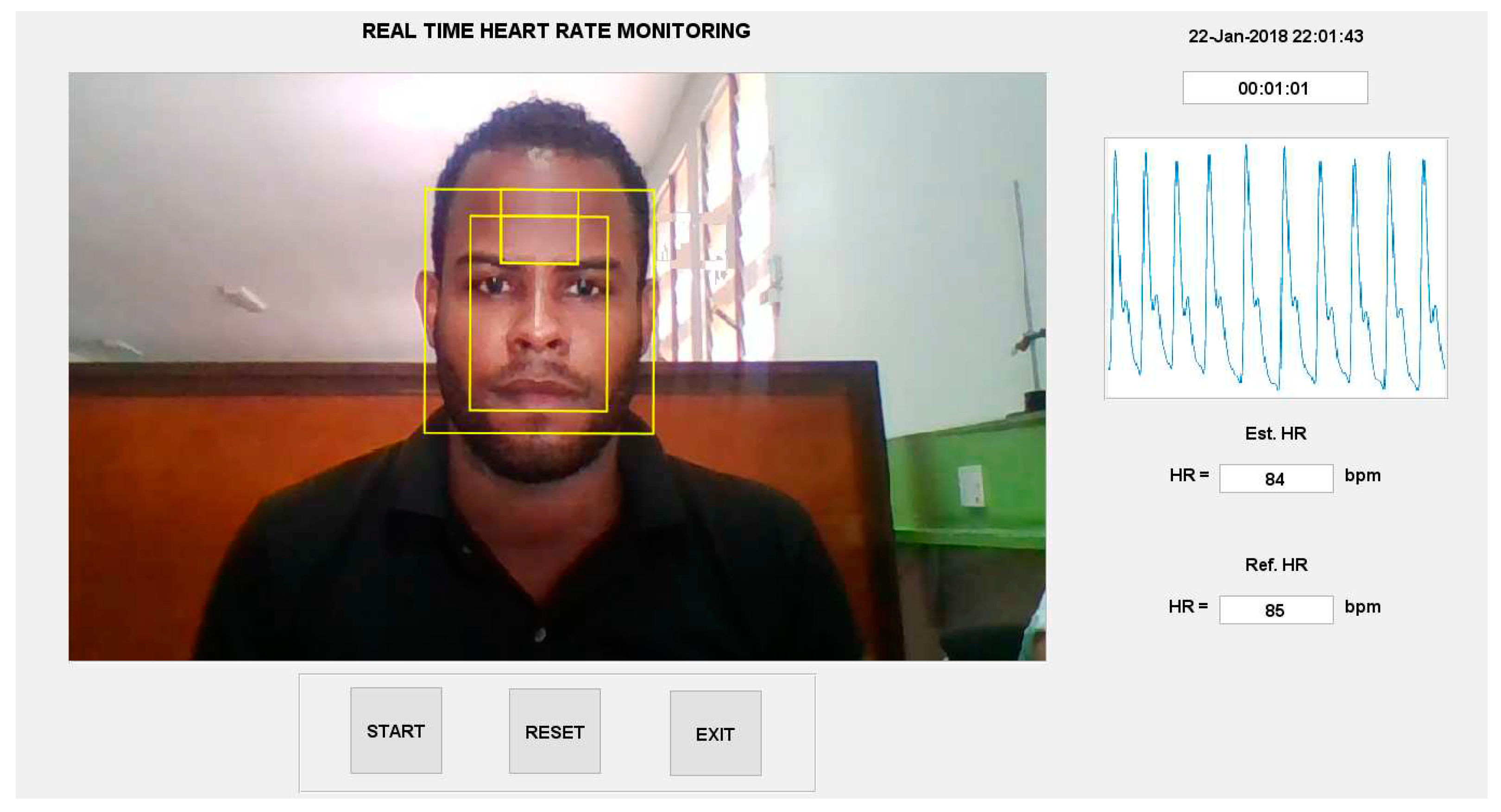
Figure 6. 2. GUI2.
Figure 6. 2. GUI2.
Preprints 69042 g043
The live video stream (with processing features such as the bounding boxes of ROIs) is displayed in the largest panel. During processing (i.e., running of HR estimation algorithm), an HR estimate is outputted into a static text field every 15 s. The corresponding ground truth HR is also displayed in a static text field. Pressing START reconfigures the START pushbutton into a STOP pushbutton for synchronized termination of video capture and processing, the timer object and the continuous display of the ground truth signal. The RESET button resets the system for another video capture and processing event. The EXIT button performs garbage collection and closes the GUI figure. There is also a static text field for date and time of the video capture. All HR estimates and corresponding ground truths are automatically outputted to a file named by date and time of video capture. A fuller description of the functionality of GUI2 will be provided in Appendix C where the GUI will serve as the interface for a laboratory experiment centred on HR estimation by video-based rPPG.

6.7. Prepare a Laboratory Practical Centred on HR Estimation by rPPG

The GUIs discussed in Section 6.6 will serve as the interface for an experiment centred on HR estimation by rPPG. The objectives of this experiment are to:
  • To provide students an introduction to the MATLAB IDE
  • To provide students experience with extracting a clinically relevant biosignal (rPPG) using a video-based method
  • To provide students an introduction to signal processing and signal processing algorithms such as the FFT
  • To provide students the opportunity to perform simple statistical analyses on data
A full description of the laboratory exercise is provided in Appendix C.

7. Conclusions and Further Work

7.1. Conclusions

An algorithmic framework for HR estimation by rPPG was successfully implemented in MATLAB. Though the results from the self-captured videos were generally poor (best case mean error of 22%), they were good enough to validate the algorithmic implementation.
The COHFACE videos yielded far superior results with mean error ranging from 3% to 15% for ambient lighting and 0% to 9% for dedicated lighting. Overall for COHFACE videos, ROI B and C performed comparably in terms of mean SNR, with both outperforming ROI A. ROI B is, however, likely to prove more robust than ROI C under significant motion. The luminance signal proved inferior to its green equivalent in terms of both mean SNR and mean error. While its mean SNR values (FFT) were 0.26 (ambient lighting) and 0.43 (dedicated lighting), corresponding values for its green counterpart were 0.27 and 0.55. Similarly, while the mean error values (FFT) for the luminance signal were 15% (ambient lighting) and 2% (dedicated lighting), corresponding values for the green signal were 8% and 1%. Performance metrics of rPPG signals were far superior under dedicated lighting (relative to ambient) with mean error reductions ranging from 25% to 100% and mean SNR increases ranging from to 59% to 104%. In keeping with research objectives 6 and 7, the HR estimation algorithm was successfully implemented within a GUI; it serves as the interface for an rPPG lab exercise detailed in Appendix C.

7.2. Further Work

This research project sets a foundation for further investigation. Possible future work includes:
Better ROI selection: ROI selection based on a skin mask from which non-rigid structures of the face (mouth, eyes) have been removed. This should lead to an improvement in SNR as it maximizes the number of skin pixels and reduces motion-based noise.
Better motion tracking: periodic re-detection of the face to minimize effect of ROI drift due to suboptimal tracking by KLT algorithm
Use of cleanest signal: for SNR and accuracy comparison with original signal; this can be accomplished by taking the 30 s sub-trace of original signal with minimum outliers
Use of PCA or ICA: to assist with denoising
Evaluation of extent of noise due to fluctuations in background lighting
Prospective further correction for suboptimal tracking: by the development of a technique based on evaluating the time series of the coordinates of the face detector bounding box
Test of comparative SNR performance of various orthogonal signals in RGB and other color spaces: based on the findings of Sahindrakar et al. that signal X = R – G + 2B outperforms the green RGB signal in SNR (2011)
Pooling of best practices for SNR optimization: to improve accuracy of HR estimation for dark-skinned subjects
Further investigation of the viability of the summary autocorrelation function (SACF): for improving the SNR of rPPG signals

Acknowledgements

I want to thank my primary supervisor, Dr. Andre Coy, for his continual guidance and assistance with research materials. I also want to thank my secondary supervisor, Professor Mitko Voutchkov, for his frequent advice and for recommending that I work with Dr. Coy. Special thanks are due to my friend, Dr. Adwalia Fevrier-Paul, for her advice and abundant support, and for performing all ground truth heart rate measurements for the self-captured videos.

Dedication

This thesis is dedicated to my father, who, in support of his family, has lived a sacrificial life; and my mother, whose mere existence, is a significant source of strength.

List of Acronyms

Acronym Expansion
AC Alternating Current
AVI Audio Video Interleaved
bpm beats per minute
BR Breathing Rate
BVP Blood Volume Pulse
CCD Charge-Coupled Device
CMOS Complementary Metal-Oxide-Semiconductor
COHFACE COntactless Heartbeat detection for trustworthy FACE Biometrics
COG Cyan, Orange and Green
DC Direct Current
DFT Discrete Fourier Transform
ECG Electrocardiograph, Electrocardiography, Electrocardiogram
FFT Fast Fourier Transform
fps frames per second
FWHM Full Width at Half Maximum
GUI Graphical User Interface
HDF5 Hierarchical Data Format 5
HeNe Helium-Neon
HR Heart Rate
HRV Heart Rate Variability
ICA Independent Component Analysis
ICU Intensive Care Unit
IDE Integrated Development Environment
JADE Joint Approximation Diagonalization of Eigen-matrices
KLT Kanade-Lucas-Tomasi
LED Light Emitting Diode
MATLAB Matrix Laboratory
MP4 MPEG-4 Part 14
mW milliwatt
PCA Principal Component Analysis
PPG Photoplethysmography
RGB Red, Green and Blue
RMSE Root-Mean-Square Error
rPPG Reflectance Photoplethysmography
SACF Summary Autocorrelation Function
SNR Signal-to-Noise Ratio
SPA Smoothness Priors Approach
SaO2 arterial Oxygen Saturation
YCbCr Luminance, blue-difference Chroma, and red-difference Chroma

Appendix A. Raw Results

Table A1. Self-captured videos – rPPG HR estimates (max peak, ambient lighting).
Video Heart Rate Estimate Ref. HR
SIG1 SIG2 SIG3 SIG4
FFT Welch FFT Welch FFT Welch FFT Welch
1 83.60 84.96 83.60 207.30 83.60 234.49 83.60 84.96 85
2 209.50 207.30 101.84 101.95 101.84 207.30 87.29 88.36 88
3 74.68 173.32 174.68 81.56 174.68 173.32 174.68 84.96 86
4 83.36 108.75 106.63 108.75 170.61 108.75 83.36 84.96 85
5 19.42 220.90 224.21 241.29 247.20 248.09 115.94 84.96 86
6 45.66 149.53 103.90 129.14 239.83 241.29 149.53 149.53 83
7 89.40 91.41 135.60 112.50 90.40 91.41 89.40 98.44 86
8 13.40 169.92 170.91 169.92 130.36 129.14 183.46 183.52 97
9 14.89 116.02 115.90 116.02 184.43 116.02 180.40 179.30 97
10 17.14 217.50 241.37 241.29 217.14 217.50 237.49 237.89 94
11 121.92 122.34 176.54 122.34 199.94 200.51 92.66 95.16 95
12 114.38 115.55 114.38 115.55 114.38 115.55 100.81 101.95 100
13 148.87 142.73 94.73 142.73 147.90 142.73 98.60 98.55 100
14 118.00 251.48 118.00 115.55 132.51 251.48 193.44 193.71 97
15 99.04 173.32 99.04 98.55 173.81 173.32 99.04 98.55 98
16 194.41 163.13 194.41 163.13 213.85 214.10 103.04 101.95 106
17 02.19 241.29 189.55 142.73 202.19 305.86 105.96 105.35 107
18 173.61 173.32 173.61 173.32 113.48 112.15 101.84 101.95 104
19 248.71 251.48 150.00 149.53 248.71 125.74 210.97 207.30 107
20 100.50 101.95 100.50 101.95 100.50 101.95 149.75 105.47 104
21 152.68 152.93 140.20 180.12 152.68 152.93 178.61 98.55 99
22 181.94 183.52 249.68 129.14 182.90 183.52 96.77 95.16 100
23 204.88 146.13 148.56 146.13 204.88 203.91 102.92 98.55 100
24 315.66 129.14 128.96 227.70 315.66 200.51 100.09 98.55 101
25 181.57 180.12 156.33 156.33 142.73 142.73 98.07 135.94 99
26 105.00 105.47 105.00 112.50 105.00 105.47 150.00 151.17 130
27 174.87 176.72 174.87 81.56 175.85 176.72 107.84 159.73 111
28 137.50 139.34 149.12 139.34 137.50 139.34 137.50 139.34 143
29 238.02 237.89 238.02 237.89 238.99 237.89 123.38 122.34 127
30 309.81 309.26 117.88 115.55 173.42 173.32 117.88 118.95 121
31 241.24 256.64 185.57 179.30 167.99 249.61 83.02 84.38 87
32 103.64 94.92 103.64 172.27 103.64 80.86 91.91 91.41 83
33 284.00 284.77 80.30 80.86 284.98 284.77 80.30 80.86 82
34 322.90 214.45 88.33 87.89 159.00 214.45 88.33 87.89 87
35 79.72 94.92 79.72 80.86 126.95 126.56 126.95 161.72 81
36 334.13 305.86 117.58 84.38 220.47 305.86 83.29 84.38 87
37 238.50 130.08 89.31 91.41 238.50 288.28 172.74 94.92 85
38 240.72 168.75 312.45 168.75 240.72 232.03 240.72 239.06 83
39 107.67 84.96 115.36 129.14 107.67 108.75 94.21 105.35 87
40 189.63 105.47 130.68 130.08 225.00 225.00 84.50 91.41 87
41 241.18 172.27 169.61 158.20 241.18 239.06 235.29 235.55 84
42 232.48 232.03 204.03 203.91 290.35 288.28 177.55 175.78 85
43 212.73 214.10 191.74 214.10 211.78 214.10 165.03 197.11 83
44 272.46 274.22 283.28 284.77 354.10 281.25 240.00 239.06 81
45 223.30 227.70 198.69 197.11 283.85 282.07 292.37 292.27 83
46 290.51 239.06 80.48 123.05 240.46 239.06 299.35 161.72 84
47 314.07 158.20 159.00 158.20 326.83 326.95 180.59 179.30 83
48 218.27 217.97 283.85 217.97 218.27 217.97 240.78 210.94 80
49 173.75 203.91 300.65 221.48 300.65 281.25 240.13 179.30 87
50 233.26 234.49 322.40 81.56 233.26 234.49 233.26 146.13 83
Table A2. Self-captured videos – rPPG HR estimates (sig. peak, ambient lighting).
Video Heart Rate Estimate Ref. HR
SIG1 SIG2 SIG3 SIG4
FFT Welch FFT Welch FFT Welch FFT Welch
1 83.60 84.96 83.60 84.96 83.60 84.96 83.60 84.96 85
2 87.29 88.36 87.29 88.36 87.29 88.36 87.29 88.36 88
3 84.43 81.56 84.43 81.56 84.43 81.56 84.43 84.96 86
4 83.36 84.96 83.36 84.96 83.36 84.96 83.36 84.96 85
5 86.23 84.96 86.23 84.96 86.23 84.96 86.23 84.96 86
6 84.48 84.96 84.48 84.96 84.48 84.96 84.48 84.96 83
7 81.36 80.86 81.36 80.86 81.36 80.86 81.36 80.86 86
8 94.63 95.16 94.63 95.16 94.63 95.16 94.63 95.16 97
9 95.74 98.44 95.74 98.44 95.74 98.44 95.74 98.44 97
10 92.09 91.76 92.09 91.76 92.09 91.73 92.09 91.73 94
11 92.66 95.16 92.66 95.16 92.66 95.16 92.66 95.16 95
12 100.80 102.00 100.80 102.00 100.80 102.00 100.80 102.00 100
13 94.73 95.16 94.73 95.16 94.73 95.16 98.60 98.55 100
14 97.69 95.16 97.69 95.16 97.69 95.16 97.69 95.16 97
15 99.04 98.55 99.04 98.55 99.04 98.55 99.04 98.55 98
16 103.00 102.00 103.00 102.00 103.00 102.00 103.00 102.00 106
17 106.00 105.40 106.00 105.40 106.00 105.40 106.00 105.40 107
18 101.80 102.00 101.80 102.00 101.80 102.00 101.80 102.00 104
19 106.50 105.40 106.50 105.40 106.50 105.40 106.50 105.40 107
20 100.50 102.00 100.50 102.00 100.50 102.00 100.50 102.00 104
21 98.91 98.55 98.91 98.55 98.91 98.55 98.91 98.55 99
22 96.77 98.55 96.77 98.55 96.77 98.55 96.77 95.16 100
23 102.90 98.55 102.90 98.55 102.90 98.55 102.90 98.55 100
24 100.10 98.55 100.10 98.55 100.10 98.55 100.10 98.55 101
25 98.07 98.55 98.07 98.55 98.07 98.55 98.07 98.55 99
26 126.00 126.60 126.00 126.60 126.00 126.60 126.00 126.60 130
27 107.80 108.80 107.80 108.80 107.80 108.80 107.80 108.80 111
28 137.50 139.30 137.50 139.30 137.50 139.30 137.50 139.30 143
29 123.40 122.30 123.40 122.30 123.40 122.30 123.40 122.30 127
30 117.90 118.90 117.90 118.90 117.90 118.90 117.90 118.90 121
31 83.02 84.38 83.02 84.38 83.02 84.38 83.02 84.38 87
32 81.15 80.86 81.15 80.86 81.15 80.86 81.15 80.86 83
33 80.30 80.86 80.30 80.86 80.30 80.86 80.30 80.86 82
34 88.33 87.89 88.33 87.89 88.33 87.89 88.33 87.89 87
35 79.72 80.86 79.72 80.86 79.72 80.86 79.72 80.86 81
36 84.27 84.38 84.27 84.38 84.27 84.38 84.27 84.38 87
37 80.48 77.34 80.48 77.34 80.48 77.34 80.48 77.34 85
38 83.52 84.38 83.52 84.38 83.52 84.38 83.52 84.38 83
39 84.60 84.96 84.60 84.96 82.67 84.96 82.67 84.96 87
40 84.50 84.38 84.50 84.38 84.50 84.38 84.50 84.38 87
41 83.33 84.38 83.33 84.38 83.33 84.38 83.33 84.38 84
42 83.38 84.38 83.38 84.38 83.38 84.38 83.38 84.38 85
43 79.18 81.56 79.18 81.56 79.18 81.56 79.18 81.56 83
44 80.66 80.86 80.66 80.86 80.66 80.86 80.66 80.86 81
45 80.42 81.56 80.42 81.56 80.42 81.56 80.42 81.56 83
46 80.48 80.86 80.48 80.86 80.48 80.86 80.48 80.86 84
47 80.48 80.86 80.48 80.86 80.48 80.86 80.48 80.86 83
48 78.30 77.34 78.30 77.34 78.30 77.34 78.30 77.34 80
49 88.83 87.89 88.83 87.89 88.83 87.89 88.83 87.89 87
50 81.55 81.56 81.55 81.56 81.55 81.56 81.55 81.56 83
Table A3. Self-captured videos – rPPG HR estimates (max peak, dedicated lighting).
Video Heart Rate Estimate Ref. HR
SIG1 SIG2 SIG3 SIG4
FFT Welch FFT Welch FFT Welch FFT Welch
1 226.96 95.16 131.91 95.16 226.96 95.16 93.11 91.76 95
2 155.62 190.31 187.47 186.91 189.29 190.31 95.55 95.16 98
3 279.99 98.55 96.88 98.55 153.07 98.55 96.88 98.55 100
4 120.20 142.73 92.09 142.73 142.50 142.73 101.78 101.95 99
5 238.24 95.16 94.52 95.16 140.82 190.31 96.45 95.16 94
6 91.98 91.76 91.98 91.76 91.98 91.76 183.96 95.16 91
7 217.01 217.50 217.01 217.50 230.64 231.09 97.32 95.16 94
8 134.37 176.72 263.90 180.12 182.70 183.52 88.93 91.76 92
9 210.29 210.94 189.16 158.20 86.53 210.94 101.62 214.45 94
10 101.15 101.95 101.15 101.95 98.23 98.55 95.32 95.16 96
11 120.13 118.95 120.13 118.95 120.13 118.95 120.13 118.95 122
12 287.14 285.47 121.15 118.95 286.18 285.47 114.47 115.55 119
13 182.50 152.93 115.87 115.55 231.74 231.09 115.87 115.55 119
14 110.80 135.94 103.09 105.35 110.80 142.73 110.80 108.75 112
15 118.00 217.50 79.31 217.50 241.80 241.29 109.29 108.75 113
16 110.51 108.75 110.51 108.75 109.54 108.75 110.51 108.75 112
17 163.61 105.35 115.49 105.35 163.61 278.67 115.49 115.55 112
18 115.30 116.02 115.30 116.02 115.30 116.02 117.28 116.02 113
19 148.23 118.95 110.45 118.95 217.98 149.53 110.45 112.15 110
20 127.88 282.07 134.67 129.14 190.86 190.31 102.69 101.95 107
21 141.28 142.73 267.69 271.88 152.44 149.53 152.44 149.53 146
22 207.05 207.30 207.05 163.13 207.05 207.30 271.21 271.88 139
23 193.66 193.71 128.78 234.49 193.66 193.71 128.78 129.14 132
24 236.66 237.89 236.66 234.49 236.66 237.89 236.66 234.49 124
25 220.04 146.13 109.54 122.34 180.30 180.12 120.20 122.34 123
26 118.46 118.95 118.46 118.95 118.46 118.95 118.46 105.35 121
27 224.77 115.55 117.23 115.55 117.23 115.55 118.20 118.95 121
28 114.64 115.55 114.64 115.55 217.62 217.50 229.28 231.09 121
29 123.52 115.55 114.77 115.55 123.52 115.55 182.85 176.72 117
30 189.82 190.31 111.21 190.31 238.71 186.91 111.21 112.15 115
31 182.05 183.52 182.05 224.30 214.63 217.50 212.71 217.50 115
32 70.39 55.78 67.61 65.63 109.28 65.63 82.43 82.03 112
33 219.41 217.50 219.41 217.50 217.50 217.50 217.50 217.50 113
34 212.94 210.70 212.94 210.70 212.94 210.70 211.03 210.70 109
35 64.97 85.31 64.97 85.31 85.39 85.31 64.97 98.44 110
36 257.74 258.28 257.74 258.28 257.74 258.28 86.90 78.16 82
37 87.53 116.02 117.72 116.02 87.53 87.89 117.72 116.02 84
38 81.61 81.56 166.13 81.56 81.61 81.56 78.69 78.16 83
39 157.83 149.53 152.02 149.53 182.04 149.53 232.39 78.16 81
40 80.59 81.56 80.59 81.56 80.59 81.56 162.15 163.13 82
41 185.35 186.91 73.75 74.77 175.65 288.87 74.72 74.77 74
42 253.43 163.13 162.15 163.13 149.53 149.53 80.59 81.56 80
43 124.08 139.34 112.45 112.15 124.08 197.11 143.47 142.73 78
44 158.45 159.73 158.45 159.73 250.79 251.48 79.71 81.56 84
45 83.69 81.56 83.69 81.56 83.69 84.96 83.69 84.96 83
46 174.87 156.33 157.39 156.33 81.61 152.93 84.52 84.96 83
47 148.31 149.53 140.56 98.55 148.31 149.53 132.80 132.54 140
48 124.49 122.34 124.49 122.34 124.49 122.34 124.49 135.94 127
49 115.55 115.55 116.52 115.55 115.55 115.55 115.55 115.55 117
50 113.23 112.15 113.23 112.15 113.23 112.15 112.26 112.15 117
51 114.51 112.15 114.51 112.15 114.51 115.55 114.51 115.55 118
Table A4. Self-captured videos – rPPG HR estimates (sig. peak, dedicated lighting).
Video Heart Rate Estimate Ref. HR
SIG1 SIG2 SIG3 SIG4
FFT Welch FFT Welch FFT Welch FFT Welch
1 96.99 95.16 96.99 95.16 96.02 95.16 93.11 91.76 95
2 95.55 95.16 95.55 95.16 95.55 95.16 95.55 95.16 98
3 96.88 98.55 96.88 98.55 96.88 98.55 96.88 98.55 100
4 92.09 91.76 92.09 91.76 92.09 91.76 92.09 91.76 99
5 93.56 95.16 94.52 95.16 93.56 95.16 96.45 95.16 94
6 91.98 91.97 91.98 91.76 91.98 91.76 93.90 95.16 91
7 87.58 98.55 87.58 98.55 87.58 98.55 97.32 95.16 94
8 93.77 91.76 88.93 88.36 90.87 91.76 88.93 91.76 92
9 86.53 87.53 86.53 87.53 86.53 87.53 86.53 87.89 94
10 101.20 102.00 101.20 102.00 98.23 98.55 95.32 95.16 96
11 120.10 118.90 120.10 118.90 120.10 118.90 120.10 118.90 122
12 114.50 122.30 114.50 118.50 114.50 115.50 114.50 115.50 119
13 115.90 115.50 115.90 115.50 115.90 115.50 115.90 115.50 119
14 110.80 105.40 110.80 105.40 110.80 108.80 110.80 108.80 112
15 112.20 112.10 112.20 112.10 112.20 112.10 112.20 108.80 113
16 110.50 108.80 110.50 108.80 109.50 108.80 110.50 108.80 112
17 115.50 105.40 115.50 115.50 115.50 115.50 115.50 115.50 112
18 115.30 116.00 115.30 116.00 115.30 116.00 117.30 116.00 113
19 110.40 105.40 110.40 108.80 110.40 105.40 110.40 112.10 110
20 102.70 102.00 102.70 102.00 102.70 102.00 102.70 102.00 107
21 152.40 149.50 152.40 149.50 152.40 149.50 152.40 149.50 146
22 135.10 135.90 135.10 135.90 135.10 135.90 135.10 135.90 139
23 128.80 129.10 128.80 129.10 128.80 129.10 128.80 129.10 132
24 122.20 122.30 122.20 122.30 122.20 122.30 122.20 122.30 124
25 120.20 122.30 120.20 122.30 120.20 122.30 120.20 122.30 123
26 118.50 118.90 118.50 118.90 118.50 118.90 118.50 118.90 121
27 118.20 115.50 118.20 115.50 118.20 115.50 118.20 118.90 121
28 114.60 115.50 114.60 115.50 114.60 115.50 114.60 112.10 121
29 114.80 115.50 114.80 115.50 114.80 115.50 114.80 115.50 117
30 111.20 112.10 111.20 112.10 111.20 112.10 111.20 112.10 115
31 113.10 115.50 113.10 115.50 113.10 115.50 113.10 115.50 115
32 109.30 111.60 109.30 111.60 109.30 111.60 109.30 111.60 112
33 114.50 115.50 114.50 115.50 114.50 115.50 114.50 115.50 113
34 109.30 108.80 109.30 108.80 109.30 108.80 109.30 108.80 109
35 108.60 108.30 108.60 108.30 108.60 108.30 108.60 108.30 110
36 79.99 78.16 79.99 78.16 79.99 78.16 79.99 78.16 82
37 87.53 87.89 87.53 87.89 87.53 87.89 87.53 84.38 84
38 81.61 81.56 81.61 81.56 81.61 81.56 78.69 78.16 83
39 78.43 78.16 78.43 78.16 78.43 78.16 77.46 78.16 81
40 80.59 81.56 80.59 81.56 80.59 81.56 80.59 81.56 82
41 73.75 74.77 73.75 74.77 73.75 74.77 74.72 74.77 74
42 81.56 81.56 81.56 81.56 80.59 81.56 80.59 81.56 80
43 73.67 74.77 73.67 74.77 73.67 74.77 73.67 74.77 78
44 79.71 78.16 79.71 78.16 79.71 78.16 79.71 81.56 84
45 83.69 81.56 83.69 81.56 83.69 84.96 83.69 84.96 83
46 81.61 81.56 81.61 81.56 81.61 81.56 81.61 94.96 83
47 132.80 132.50 132.80 132.50 132.80 132.50 132.80 132.50 140
48 124.50 122.30 124.50 122.30 124.50 122.30 124.50 122.30 127
49 115.50 115.50 115.50 115.50 115.50 115.50 115.50 115.50 117
50 113.20 112.10 113.20 112.10 113.20 112.10 112.30 112.10 117
51 114.50 112.10 114.50 112.10 114.50 115.50 114.50 115.50 118
Table A5. COHFACE videos – rPPG HR estimates (ambient lighting).
Video Heart Rate Estimate Ref. HR
SIG1 SIG2 SIG3 SIG4
FFT Welch FFT Welch FFT Welch FFT Welch
1* 82.45 82.03 82.45 82.03 82.45 84.38 82.45 82.03 82.48
2 80.53 79.69 75.56 79.69 81.52 79.69 78.54 79.69 81.49
3 70.53 84.38 117.22 117.19 70.53 70.31 70.53 70.31 70.49
4 70.47 70.31 70.47 70.31 70.47 70.31 70.47 70.31 70.41
5 72.52 70.31 72.52 70.31 72.52 72.66 71.52 72.66 72.40
6 130.13 93.75 130.13 128.91 95.36 128.91 131.13 121.88 71.48
7 93.38 93.75 93.38 93.75 53.64 93.75 106.29 107.81 53.55
8 54.55 53.91 54.55 53.91 54.55 53.91 54.55 53.91 54.55
9 67.21 67.97 67.21 67.97 67.21 67.97 67.21 67.97 67.11
10 68.60 67.97 67.63 67.97 68.60 67.97 67.63 67.97 68.50
11 61.59 60.94 61.59 60.94 59.60 60.94 59.60 91.41 61.55
12 65.51 65.63 65.51 65.63 65.51 65.63 65.51 65.63 65.45
13 75.37 75.00 75.37 75.00 75.37 75.00 75.37 75.00 75.27
14 78.14 77.34 78.14 77.34 78.14 77.34 78.14 77.34 78.07
15 70.36 70.31 70.36 70.31 70.36 67.97 70.36 70.31 70.27
16 68.43 67.97 68.43 67.97 68.43 67.97 68.43 67.97 68.36
17 91.47 135.94 91.47 91.41 92.46 93.75 91.47 91.41 91.33
18 88.05 89.06 89.04 89.06 88.05 86.72 87.06 86.72 87.99
19 61.49 60.94 61.49 60.94 61.49 60.94 61.49 60.94 61.42
20 62.43 63.28 62.43 63.28 62.43 63.28 62.43 63.28 62.35
21 82.45 82.03 82.45 82.03 83.44 82.03 82.45 82.03 83.39
22 82.52 84.38 82.52 84.38 85.50 84.38 85.50 84.38 85.38
23 80.20 173.44 66.34 65.63 93.07 93.75 91.09 93.75 90.96
24 76.49 145.31 169.87 77.34 108.28 107.81 89.40 89.06 89.26
*Pairs of consecutive Video number refer to the same subject. For example, Video 1 and 2 belong to subject 1, while 3 and 4 belong to subject 2.
Table A6. COHFACE videos – rPPG HR estimates (dedicated lighting).
Video Heart Rate Estimate Ref. HR
SIG1 SIG2 SIG3 SIG4
FFT Welch FFT Welch FFT Welch FFT Welch
1 84.65 84.38 84.65 84.38 84.65 84.38 84.65 84.38 84.56
2 85.50 86.72 85.50 86.72 85.50 86.72 85.50 84.38 85.47
3 69.54 70.31 69.54 70.31 69.54 70.31 69.54 70.31 69.49
4 68.54 67.97 68.54 67.97 68.54 67.97 68.54 67.97 68.43
5 68.60 67.97 68.60 67.97 68.60 67.97 68.60 67.97 68.50
6 70.30 70.31 70.30 70.31 70.30 70.31 70.30 70.31 70.27
7 57.57 56.25 57.57 56.25 57.57 56.25 56.58 56.25 56.53
8 53.69 53.91 53.69 110.16 53.69 53.91 53.69 56.25 53.61
9 71.34 70.31 71.34 70.31 71.34 70.31 71.34 70.31 71.22
10 69.16 67.97 69.16 67.97 69.16 67.97 69.16 67.97 69.06
11 59.55 60.94 59.55 84.38 59.55 58.59 59.55 60.94 59.50
12 64.52 63.28 64.52 63.28 60.55 63.28 60.55 60.94 60.50
13 75.30 77.34 75.30 77.34 75.30 77.34 76.27 77.34 76.22
14 74.58 75.00 74.58 75.00 74.58 75.00 74.58 75.00 74.52
15 67.49 67.97 67.49 67.97 67.49 67.97 67.49 67.97 67.44
16 69.48 70.31 69.48 70.31 69.48 70.31 69.48 70.31 69.42
17 86.42 86.72 78.48 84.38 78.48 84.38 85.43 84.38 86.28
18 83.44 84.38 83.44 82.03 83.44 84.38 83.44 84.38 83.31
19 60.55 58.59 60.55 58.59 60.55 60.94 60.55 60.94 60.50
20 61.49 60.94 61.49 60.94 61.49 60.94 61.49 60.94 61.42
21 81.46 82.03 81.46 82.03 81.46 82.03 80.46 82.03 80.41
22 84.30 84.38 84.30 84.38 84.30 84.38 84.30 84.38 84.21
23 94.29 93.75 119.11 119.53 94.29 93.75 94.29 93.75 95.21
24 96.44 75.00 96.44 96.09 96.44 96.09 88.48 89.06 89.35

Appendix B. HR Estimation Algorithm

%STAGE 1: DETECT A FACE
% Create a cascade detector object.
faceDetector = vision.CascadeObjectDetector();
% Read a video frame and run the face detector.
videoFileReader = vision.VideoFileReader(NAME4);
videoFrame = step(videoFileReader);
bbox = step(faceDetector, videoFrame);
fROI = [(bbox(1) + (1/3)*bbox(3)) (bbox(2) + 0.1*bbox(4)) ((1/3)*bbox(3)) (0.2*(bbox(4)))];
bfROI= [(bbox(1) + (1/3)*bbox(3)) (bbox(2) + 0.0*bbox(4)) ((1/3)*bbox(3)) (0.3*(bbox(4)))];
bbROI=[(bbox(1) + (0.2)*bbox(3)) (bbox(2) + 0.1*bbox(4)) ((0.6)*bbox(3)) (0.8*(bbox(4)))];
fROIPoints = bbox2points(fROI(1, :));
bfROIPoints = bbox2points(bfROI(1, :));
bbROIPoints = bbox2points(bbROI(1, :));
redChannel = videoFrame(:, :, 1); % red channel of video frame
greenChannel = videoFrame(:, :, 2); % green channel of video frame
blueChannel = videoFrame(:, :, 3); % blue channel of video frame
YCbCr = rgb2ycbcr(videoFrame);
YChannel = YCbCr(:,:,1);
x1 = fROIPoints(:,1);
y1 = fROIPoints(:,2);
x2 = bfROIPoints(:,1);
y2 = bfROIPoints(:,2);
x3 = bbROIPoints(:,1);
y3 = bbROIPoints(:,2);
bw1 = poly2mask(x1, y1, size(videoFrame, 1), size(videoFrame, 2)); % creates binary mask based on polygon with vetices defined by x and y with vid frame dimensions
bw2 = poly2mask(x2, y2, size(videoFrame, 1), size(videoFrame, 2));
bw3 = poly2mask(x3, y3, size(videoFrame, 1), size(videoFrame, 2));
p = 1;
pSIG1(1, p) = mean2(redChannel(logical(bw1))); %bigger forehead ROI raw red signal vector
pSIG2(1, p) = mean2(greenChannel(logical(bw1))); %bigger forehead ROI raw green signal vector
pSIG3(1, p) = mean2(blueChannel(logical(bw1))); %bigger forehead ROI raw blue signal vector
pSIG4(1, p) = mean2(YChannel(logical(bw1))); %bigger forehead ROI raw luminance signal vector
pSIG5(1, p) = mean2(greenChannel(logical(bw2))); % bigger forehead ROI raw green signal vector
pSIG6(1, p) = mean2(greenChannel(logical(bw3))); % 60%80% bounding box ROI raw green signal vector
pSIG9(1, p) = fROIPoints(1,1); % x motion signal from first x coordinate of forehead ROI
pSIG10(1, p) = fROIPoints(1,2); % y motion signal from first y coordinate of forehead ROI
% Draw the returned bounding box around the detected face.
videoFrame = insertShape(videoFrame, ‘Rectangle’, bbox);
videoFrame = insertShape(videoFrame, ‘Rectangle’, fROI); % insert forehead ROI into video frame
videoFrame = insertShape(videoFrame, ‘Rectangle’, bfROI);
videoFrame = insertShape(videoFrame, ‘Rectangle’, bbROI);
%figure; imshow(videoFrame); title(‘Detected face’);
% Convert the first box into a list of 4 points
% This is needed to be able to visualize the rotation of the object.
bboxPoints = bbox2points(bbox(1, :));
%fROIPoints = bbox2points(fROI(1, :)); % convert fROI to four coordinates of rectangle
% This establishes the ROI in first frame; the bbox coordinates are transformed to yield
% the coordinates for a ROI at 60% width of bbox and 80% height; assumes that bounding box in
% first frame is (unrotated) square/rectangle
%STAGE 2: IDENTIFY FACIAL FEATURES TO TRACK
% Detect feature points in the face region.
points = detectMinEigenFeatures(rgb2gray(videoFrame), ‘ROI’, bbox);
% Display the detected points.
%figure, imshow(videoFrame), hold on, title(‘Detected features’);
%plot(points);
%STAGE 3: INITIALIZE A TRACKER TO TRACK THE POINTS
% Create a point tracker and enable the bidirectional error constraint to
% make it more robust in the presence of noise and clutter.
pointTracker = vision.PointTracker(‘MaxBidirectionalError’, 2);
% Initialize the tracker with the initial point locations and the initial
% video frame.
points = points.Location;
initialize(pointTracker, points, videoFrame);
%STAGE 4: INITIALIZE A VIDEO PLAYER TO DISPLAY THE RESULTS
videoPlayer = vision.VideoPlayer(‘Position’,...
  [100 100 [size(videoFrame, 2), size(videoFrame, 1)]+30]);
%STAGE 5: TRACK THE FACE
% Make a copy of the points to be used for computing the geometric
% transformation between the points in the previous and the current frames
oldPoints = points;
while ~isDone(videoFileReader)
  % get the next frame
  videoFrame = step(videoFileReader);
  % Track the points. Note that some points may be lost.
  [points, isFound] = step(pointTracker, videoFrame);
  visiblePoints = points(isFound, :);
  oldInliers = oldPoints(isFound, :);
  if size(visiblePoints, 1) >= 2 % need at least 2 points
    % Estimate the geometric transformation between the old points
    % and the new points and eliminate outliers
    [xform, oldInliers, visiblePoints] = estimateGeometricTransform(...
      oldInliers, visiblePoints, ‘similarity’, ‘MaxDistance’, 4);
    % Apply the transformation to the bounding box points
    bboxPoints = transformPointsForward(xform, bboxPoints);
    % Also apply the transformation to the ROI box points and other ROIs
    fROIPoints = transformPointsForward(xform, fROIPoints);
    fROIPoints = double(fROIPoints); %change fROIPoints from single to double
    bfROIPoints = transformPointsForward(xform, bfROIPoints);
    bfROIPoints = double(bfROIPoints); %change fROIPoints from single to double
    bbROIPoints = transformPointsForward(xform, bbROIPoints);
    bbROIPoints = double(bbROIPoints); %change fROIPoints from single to double
    x1 = fROIPoints(:,1);
    y1 = fROIPoints(:,2);
    x2 = bfROIPoints(:,1);
    y2 = bfROIPoints(:,2);
    x3 = bbROIPoints(:,1);
    y3 = bbROIPoints(:,2);
    
    bw1 = poly2mask(x1, y1, size(videoFrame, 1), size(videoFrame, 2));
    bw2 = poly2mask(x2, y2, size(videoFrame, 1), size(videoFrame, 2));
    bw3 = poly2mask(x3, y3, size(videoFrame, 1), size(videoFrame, 2));
    %bw4 = poly2mask(x4, y4, size(videoFrame, 1), size(videoFrame, 2));
    
    p = p + 1;
    gr(:,:,p) = fROIPoints;
    %monitor(:,:,p) = bROIPoints;
    redChannel = videoFrame(:, :, 1); % red channel of video frame
    greenChannel = videoFrame(:, :, 2); % green channel of video frame
    blueChannel = videoFrame(:, :, 3); % blue channel of video frame
    
    YCbCr = rgb2ycbcr(videoFrame);
    YChannel = YCbCr(:,:,1);
    
    pSIG1(1, p) = mean2(redChannel(logical(bw1))); %forehead ROI raw red signal
    pSIG2(1, p) = mean2(greenChannel(logical(bw1))); % forehead ROI raw green signal
    pSIG3(1, p) = mean2(blueChannel(logical(bw1))); %forehead ROI raw blue signal
    pSIG4(1, p) = mean2(YChannel(logical(bw1))); %forehead ROI raw luminance signal
    
    pSIG5(1, p) = mean2(greenChannel(logical(bw2))); % bforehead ROI raw green signal
    pSIG6(1, p) = mean2(greenChannel(logical(bw3))); % 60%80% bb box ROI raw green
    
    pSIG9(1, p) = fROIPoints(1,1); % x motion signal of forehead ROI
    pSIG10(1, p) = fROIPoints(1,2); % y motion signal of forehead ROI
    
    % Insert a bounding box around the object being tracked
    bboxPolygon = reshape(bboxPoints’, 1, []);
    videoFrame = insertShape(videoFrame, ‘Polygon’, bboxPolygon, ...
      ‘LineWidth’, 2);
    
    % Also insert fROI box around the object being tracked, and insert for other Roys
    
    fROIPolygon = reshape(fROIPoints’, 1, []);
    videoFrame = insertShape(videoFrame, ‘Polygon’, fROIPolygon, ...
      ‘LineWidth’, 2);
    
    bfROIPolygon = reshape(bfROIPoints’, 1, []);
    videoFrame = insertShape(videoFrame, ‘Polygon’, bfROIPolygon, ...
      ‘LineWidth’, 2);
    bbROIPolygon = reshape(bbROIPoints’, 1, []);
    videoFrame = insertShape(videoFrame, ‘Polygon’, bbROIPolygon, ...
      ‘LineWidth’, 2);
    
    % Display tracked points
    videoFrame = insertMarker(videoFrame, visiblePoints, ‘+’, ...
      ‘Color’, ‘white’);
    
    % Reset the points
    oldPoints = visiblePoints;
    setPoints(pointTracker, oldPoints);
  end
  % Display the annotated video frame using the video player object
  step(videoPlayer, videoFrame);
  %break
end
% Clean up
release(videoFileReader);
release(videoPlayer);
release(pointTracker);
% STEP 6: SIGNAL DETRENDING, SPA
pSIG1 = double(pSIG1’);
pSIG2 = double(pSIG2’);
pSIG3 = double(pSIG3’);
pSIG4 = double(pSIG4’);
pSIG5 = double(pSIG5’);
pSIG6 = double(pSIG6’);
pSIG9 = double(pSIG9’);
pSIG10 = double(pSIG10’);
T = length(pSIG1);
lambda = 10;
I = speye(T);
D2 = spdiags(ones(T-2,1)*[1 -2 1],[0:2],T-2,T);
dpSIG1 = (I-inv(I+lambda^2*D2’*D2))*pSIG1;
dpSIG2 = (I-inv(I+lambda^2*D2’*D2))*pSIG2;
dpSIG3 = (I-inv(I+lambda^2*D2’*D2))*pSIG3;
dpSIG4 = (I-inv(I+lambda^2*D2’*D2))*pSIG4;
dpSIG5 = (I-inv(I+lambda^2*D2’*D2))*pSIG5;
dpSIG6 = (I-inv(I+lambda^2*D2’*D2))*pSIG6;
dpSIG9 = (I-inv(I+lambda^2*D2’*D2))*pSIG9;
dpSIG10 = (I-inv(I+lambda^2*D2’*D2))*pSIG10;
% STEP 7: FILTERING
fs = 29;
[b, a] = butter(4, [0.8 6.0]/(fs/2), ‘bandpass’);
fpSIG1 = filter(b, a, dpSIG1);
fpSIG2 = filter(b, a, dpSIG2);
fpSIG3 = filter(b, a, dpSIG3);
fpSIG4 = filter(b, a, dpSIG4);
fpSIG5 = filter(b, a, dpSIG5);
fpSIG6 = filter(b, a, dpSIG6);
fpSIG9 = filter(b, a, dpSIG9);
fpSIG10 = filter(b, a, dpSIG10);
% STEP 8: SIGNAL NORMALIZATION
npSIG1 = (fpSIG1 - mean(fpSIG1))/std(fpSIG1); % remember to change these signals back to fSIG
npSIG2 = (fpSIG2 - mean(fpSIG2))/std(fpSIG2);
npSIG3 = (fpSIG3 - mean(fpSIG3))/std(fpSIG3);
npSIG4 = (fpSIG4 - mean(fpSIG4))/std(fpSIG4);
npSIG5 = (fpSIG5 - mean(fpSIG5))/std(fpSIG5);
npSIG6 = (fpSIG6 - mean(fpSIG6))/std(fpSIG6);
npSIG9 = (fpSIG9 - mean(fpSIG9))/std(fpSIG9);
npSIG10 = (fpSIG10- mean(fpSIG10))/std(fpSIG10);
% STEP 9: FFT OF R, G, and B SIGNALS + DISPLAY OF FFT OF EACH SIGNAL
L = length(npSIG1);
winvec = hann(L);
F1 = fft(npSIG1.*winvec);
F2 = fft(npSIG2.*winvec);
F3 = fft(npSIG3.*winvec);
F4 = fft(npSIG4.*winvec);
F5 = fft(npSIG5.*winvec);
F6 = fft(npSIG6.*winvec);
F9 = fft(npSIG9.*winvec);
F10 = fft(npSIG10.*winvec);
A2 = abs(F1/L);
A1 = A2(1:L/2+1);
A1(2:end-1) = 2*A1(2:end-1);
B2 = abs(F2/L);
B1 = B2(1:L/2+1);
B1(2:end-1) = 2*B1(2:end-1);
C2 = abs(F3/L);
C1 = C2(1:L/2+1);
C1(2:end-1) = 2*C1(2:end-1);
D2 = abs(F4/L);
D1 = D2(1:L/2+1);
D1(2:end-1) = 2*D1(2:end-1);
E2 = abs(F5/L);
E1 = E2(1:L/2+1);
E1(2:end-1) = 2*E1(2:end-1);
G2 = abs(F6/L);
G1 = G2(1:L/2+1);
G1(2:end-1) = 2*G1(2:end-1);
J2 = abs(F9/L);
J1 = J2(1:L/2+1);
J1(2:end-1) = 2*J1(2:end-1);
K2 = abs(F10/L);
K1 = K2(1:L/2+1);
K1(2:end-1) = 2*K1(2:end-1);
% DISPLAY THREE FFTs
f = 60*fs*(0:(L/2))/L;
figure
subplot(2,2,1)
plot(f, B1.^2, ‘green’)
title(‘fft of green signal of forehead ROI’)
xlabel(‘f(Hz)’)
ylabel(‘Power(f)’)
subplot(2,2,2)
plot(f, D1.^2)
title(‘fft of luminance signal of forehead ROI’)
xlabel(‘f(Hz)’)
ylabel(‘Power(f)’)
subplot(2,2,3)
plot(f, E1.^2, ‘green’)
title(‘fft of green signal of bigger forehead ROI’)
xlabel(‘f(Hz)’)
ylabel(‘Power(f)’)
subplot(2,2,4)
plot(f, G1.^2, ‘green’)
title(‘fft of green signal of 60%80% bb ROI’)
xlabel(‘f(Hz)’)
ylabel(‘Power(f)’)
figure
subplot(2,2,1)
plot(f, J1.^2)
title(‘fft of x motion signal’)
xlabel(‘f(Hz)’)
ylabel(‘Power(f)’)
subplot(2,2,2)
plot(f, K1.^2)
title(‘fft of y motion signal’)
xlabel(‘f(Hz)’)
ylabel(‘Power(f)’)
%------------------------------WELCH
[pxx1 f] = pwelch(npSIG2.*winvec, [], [], [], fs);
[pxx2 f] = pwelch(npSIG4.*winvec, [], [], [], fs);
[pxx3 f] = pwelch(npSIG5.*winvec, [], [], [], fs);
[pxx4 f] = pwelch(npSIG6.*winvec, [], [], [], fs);
[pxx7 f] = pwelch(npSIG9.*winvec, [], [], [], fs);
[pxx8 f] = pwelch(npSIG10.*winvec, [], [], [], fs);
figure
subplot(2,2,1)
plot(60*f, pxx1, ‘green’)
title(‘Welch of green signal of forehead ROI’)
xlabel(‘f(Hz)’)
ylabel(‘Power(f)’)
subplot(2,2,2)
plot(60*f, pxx2)
title(‘Welch of luminance signal of forehead ROI’)
xlabel(‘f(Hz)’)
ylabel(‘Power(f)’)
subplot(2,2,3)
plot(60*f, pxx3, ‘green’)
title(‘Welch of green signal of bigger forehead ROI’)
xlabel(‘f(Hz)’)
ylabel(‘Power(f)’)
subplot(2,2,4)
plot(60*f, pxx4, ‘green’)
title(‘Welch of green signal of 60%80% bb ROI’)
xlabel(‘f(Hz)’)
ylabel(‘Power(f)’)

Appendix C. Laboratory Practical

Heart Rate Estimation by Video-based Reflectance Photoplethysmography (rPPG)
Student Worksheet
In this experiment you will estimate your heart rate by extracting and processing reflectance photoplethysmography (rPPG) signals from video.
Theory
Plethysmography is the measurement and recording of changes in the volume of an organ or other body part. Photoplethysmography (PPG), as the prefix implies, is plethysmography by optical means. It is the operational basis of pulse oximetry and is often used for blood volume/pressure measurements and assessment of blood flow. The fundamental theory of PPG is that pulsatile variations in tissue blood volume modulate the transmission or reflection of visible (or infra-red) light. This is because haemoglobin, the blood-oxygen transport protein, is strongly absorptive in visible and near-infrared light. The greater the tissue blood volume, the higher the haemoglobin content and the greater the light absorption (lower the transmission and reflection). Accordingly, oscillations in tissue blood volume during the cardiac cycle produce corresponding oscillations in the transmission (or reflection) of light in synchrony with the heartbeat. The variation in the intensity of transmitted or reflected light is known as a photoplethysmographic (PPG) signal. The heart rate may be extracted from the PPG signal by measuring the time between consecutive peaks (or troughs) of the PPG waveform or, alternatively, using spectral analysis techniques such as the fast Fourier transform (FFT) and Welch periodogram.
Figure 1. Characteristic PPG signal from pulse oximeter.
Preprints 69042 g0a1
A PPG signal can be obtained from any vascular area on the skin using optical probes in either reflection or transmission mode. After the light is transmitted through or reflected from vascular tissue, it reaches a photodetector and is transduced into current variations which are then amplified and sampled to generate the PPG signal.
Figure 2. Transmission (left) and reflection (right) mode PPG.
Preprints 69042 g0a2
This experiment makes use of video-based reflectance PPG (rPPG), which is simply PPG in which light reflected from the skin is recorded by a video camera. A total of 8 rPPG signals are extracted from 3 regions of interest (ROIs). These signals are classified based on ROI, color space component (green RGB or luminance YCbCr) and spectral analysis technique (FFT or Welch periodogram). Figure 3 displays the ROIs (ROI A, B and C) while Table 1 provides a description of the ROIs and their associated signals. Referring to Table 1, signal 2.2 (extracted from ROI B), is described as: Luminance (YCbCr) signal (Welch). This means that is extracted from the luminance (Y) component of the YCbCr color space and transformed into the frequency domain using the Welch periodogram.
rPPG signal extraction from video involves calculating the mean pixel intensity within a given ROI for each video frame in a given color space. A color space refers to a particular interpretation of a mathematical representation of color as a set of components. In an RGB (red, green, blue) color space, for example, all colors are represented in terms of components red, green and blue, while in the YCbCr color space, colors are represented in terms of a luminance (brightness) component Y and two chroma (hue) components Cb and Cr (which stand for blue-difference and red difference chroma, respectively).
Extracted rPPG signals are raw signals and need to be further processed to yield heart rate. An integral stage of processing is spectral analysis in which the rPPG signal is transformed from the time domain into the frequency domain. In this experiment, this is accomplished using two techniques: the fast Fourier Transform (FFT) and the Welch periodogram, which is an implementation of the FFT designed to smooth and denoise the input signal (as rPPG signals may be significantly contaminated by motion-based and other noise). Once the signal is represented in the frequency domain, heart rate can be determined by identifying the frequency of the peak with maximum amplitude.
ROI Description and rPPG signal classification
Figure 3. Various ROIs for rPPG signal extraction.
Preprints 69042 g0a3
Table 1. ROI description and rPPG signal classification.
ROI Name ROI Description Associated Signals Description of Signal
ROI A ROI centred on Forehead SIGNAL 1.1 Green (RGB) signal (FFT)
SIGNAL 1.2 Green (RGB) signal (Welch)
SIGNAL 2.1 Luminance (YCbCr) signal (FFT)
SIGNAL 2.2 Luminance (YCbCr) signal (Welch)
ROI B Forehead ROI 50% larger than ROI A SIGNAL 3.1 Green (RGB) signal (FFT)
SIGNAL 3.2 Green (RGB) signal (Welch)
ROI C Face ROI comprises central 60% (width) and central 80% (height) of bbox SIGNAL 3.1 Green (RGB) signal (FFT)
SIGNAL 3.2 Green (RGB) signal (Welch)
Making measurements and observations
Exercise 1: Heart rate estimation by analysis of FFT of rPPG signal
1. 
Open the MATLAB IDE by double clicking on the MATLAB shortcut icon in the desktop window
2. 
Wait for the completion of MATLAB initialization and the appearance of ready at the bottom left corner of the MATLAB window
3. 
Seat at approximately 0.5 m from the webcam (use a metre rule to measure the distance). Seat still facing the camera and ensure that field of view of the webcam is centered on your face.
4. 
Insert the tip of your index figure into the rubber case of the sensor of the pulse oximeter module (already connected to the computer). An IR LED illuminates the finger from the top while a photodetector detects transmitted light at the bottom. Place the hand on a level surface (such as table top or arm rest) and keep it steady. See Figure 4 for correct placement of finger into sensor.
5. 
Type GUI1 followed by the ENTER key into the MATLAB command window. A GUI will appear and will serve as the interface for rPPG signal extraction and the outputting of FFT results (which will be analysed for heart rate estimation).
6. 
Initiate video capture (as well as a timer and simultaneous capture of ground truth pulse oximeter signal) by pressing the START pushbutton at the top of the GUI window.
7. 
Terminate video capture after 1 min (by pressing the STOP pushbutton).
8. 
Press the SELECT VIDEO pushbutton at the top of the GUI window. This is a browse button which will allow you to select the video you just recorded and enter it into the GUI space for rPPG signal extraction.
9. 
Press the PROCESS VIDEO pushbutton adjacent to SELECT VIDEO. This will initiate the processing of the video for rPPG signal. This may take more than 5 min (depending on hardware). The immediate output of this processing will be the display of the FFT of rPPG signals 1 – 4 in four labelled panels.
10.  
The Welch periodograms of signals 1 – 4 can be accessed by pressing the WELCH pushbutton at the bottom of the GUI. Return to the FFT results is achieved by pressing the same pushbutton which is automatically reconfigured and re-labelled FFT.
11. 
Determine the heart rate (in bpm) for both the FFT and Welch periodogram results by clicking on the peak of maximum amplitude in the frequency spectrum.
12. 
An FFT and Welch periodogram of the pulse oximeter reference values is obtained by pressing the GROUND TRUTH pushbutton.
13. 
Record all results in a table like the one in the Recording and presenting your data section below (it is designed to accommodate Results from multiple subjects/videos).
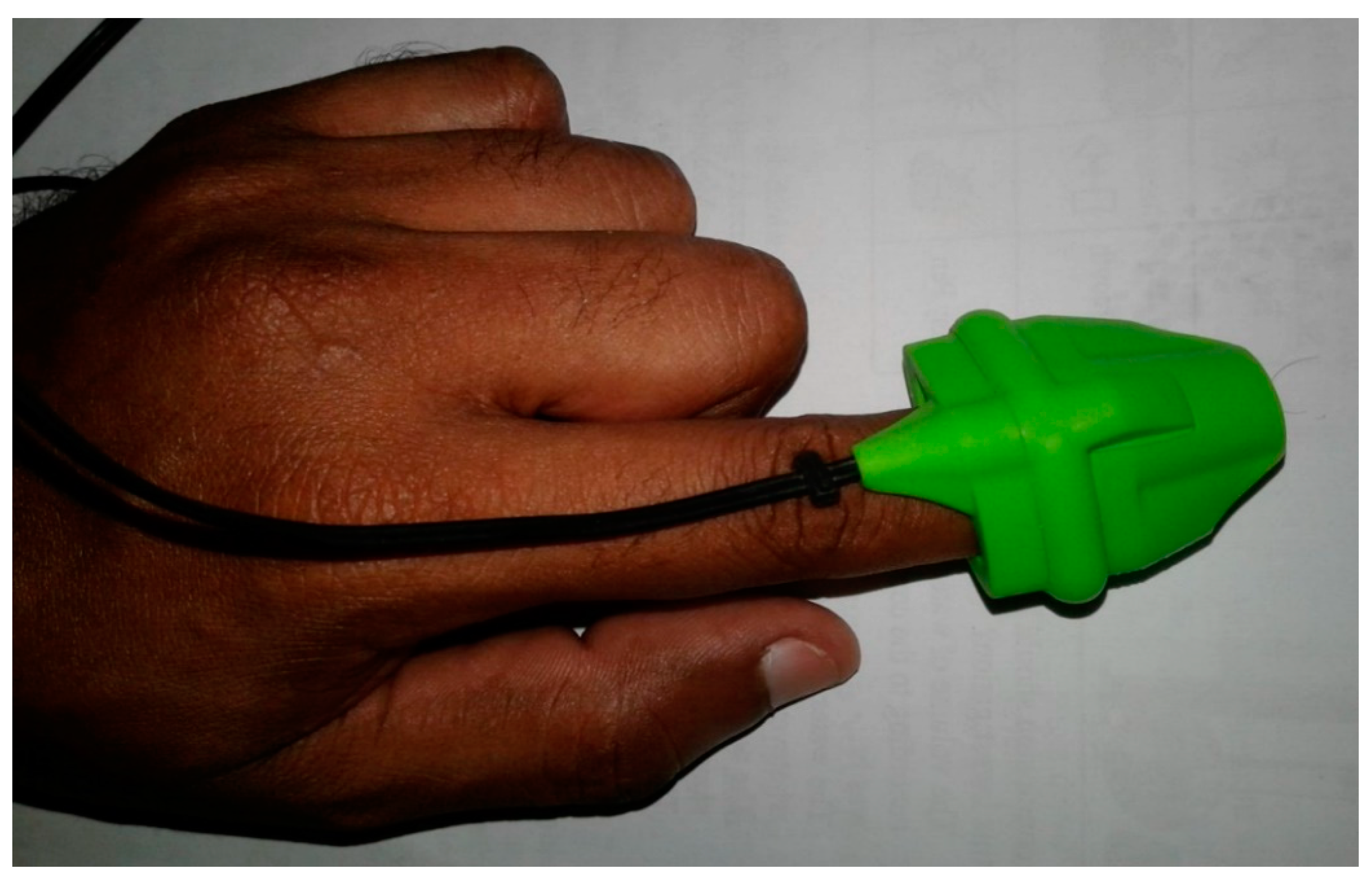
Figure 4. Placement of index finger into pulse oximeter sensor.
Preprints 69042 g0a4
Exercise 2: Calculation of Error and SNR
  • For each of the eight (8) heart rate estimates (one for each rPPG signal), you need a corresponding error and signal-to-noise ratio (SNR) measure. Error values are obtained by clicking the (static) drop-down list titled ERROR at the top of the GUI window (it allows display but no selection).
  • SNR values are obtained by clicking the adjacent SNR drop-down list.
  • Record Error and SNR values in a table like the one specified in the Recording and presenting your data section
  • Close the GUI by pressing the EXIT pushbutton and repeat steps 3 – 13 of Exercise 1 and 1 – 4 of Exercise 2 with dedicated light source about 1 metre from the face.
Exercise 3: Real-time times series of your heart rate
1. 
In the MATLAB command window, type GUI2. A new GUI will appear. Using this GUI, heart rate is determined directly without the need for manual evaluation of the FFTs.
2. 
Adopt the sitting posture employed in Exercise 1 and keep the dedicated lighting.
3. 
Press the START button at the bottom of the GUI window. Video capture will be initiated after 5 s and will yield your HR every 15 s.
4. 
Let the video run for 5 min. By then you will have 20 estimated heart rate values and 20 corresponding pulse oximeter ground truth values. These values will appear sequentially in labelled static text fields in the GUI window and will also be automatically outputted to a file.
5. 
Record your estimated HR and reference HR values in a table like the one specified in the Recording and presenting your data section
Recording and presenting your data
Exercise 1
Sample table for recording rPPG HR estimates
Video Heart Rate Estimate Ref. HR
SIG1 SIG2 SIG3 SIG4
FFT Welch FFT Welch FFT Welch FFT Welch
1
2
3
4
5
6
7
8
9
10
Exercise 2
  • Generate an Error table by reproducing the sample table for Exercise 1, replacing Heart Rate Estimates with Error in Heart Rate Estimates
  • Generate an SNR table by reproducing the sample table for Exercise 1, replacing Heart Rate Estimates with SNR
Exercise 3
Sample table for recording estimated HR vs. Ref. HR
Trial Est. HR Ref. HR
1
2
3
4
5
6
7
8
9
10
Analyzing your data
Exercise 1
1. 
Pool the class results for the HR estimates
2. 
Using the results of the FFT of signal 4, perform a correlation analysis on the heart rate determined by rPPG (est. HR) versus that measured by the pulse oximeter (ref. HR). Plot the corresponding scatter plot, indicating both the r and p value
Exercise 2
1. 
Pool the class results for error and SNR values
2. 
Calculate the mean error and mean SNR for each of the 8 rPPG signals
3. 
Plot a scatter plot of error versus SNR for the rPPG signal with the lowest mean SNR and that with the highest mean SNR. Show the r and p values on each plot
4. 
Group the error and SNR data for the class based on sex (male or female). Using the signal with the lowest mean error and that with the highest SNR, perform t-tests to determine whether there is a statistically significant difference in error and SNR between males and females. Perform the same analysis for dark-skinned versus fair-skinned subjects.
Exercise 3
1. 
Calculate the mean error for your set of 20 heart rates
2. 
Perform a correlation analysis for est. HR vs. ref. HR. Plot a corresponding scatter plot, indicating r and p values
Evaluation
1. 
What are the limits of correlation analysis and scatter plots in evaluating the relationship between est. HR and ref. HR? Is it a measure of agreement? The Bland-Altman plot may prove more useful. What are the advantages of Bland-Altman analysis over correlation analysis?
2. 
Which of the 8 rPPG signals had the lowest and highest mean SNR? What might account for this?
3. 
Which of the 8 rPPG signals had the lowest and highest mean error? What might account for this?
4. 
For the error versus SNR correlation analyses performed in Exercise 2, did the results show significant correlation? What might account for correlation between error and SNR?
5. 
For the t-tests performed in Exercise 2, was the difference in error and SNR between males and females statistically significant? What might account for a statistically significant difference? Were the differences significant for dark-skinned versus fair-skinned subjects? What might account for a statistically significant difference?
6. 
Explain how the FFT works. What other algorithm may be used for spectral analysis?
7. 
Classify the rPPG as a bio-signal
8. 
What improvements can be made to this experiment?
Heart Rate Estimation by Video-based Reflectance Photoplethysmography (rPPG)
Teaching Notes
Key learning objectives
  • To provide students an introduction to the MATLAB Integrated Development Environment (IDE)
  • To provide students experience with extracting a clinically relevant biosignals (rPPG) using a video-based method
  • To provide students an introduction to signal processing and signal processing algorithms such as the FFT
  • To provide students the opportunity to perform simple statistical analyses on data
Notes
In the case of a high percentage of low SNR rPPG signals, the experiment may be adapted to include an estimation of heart based on signal peaks (i.e., the peak which actually represents the heart rate, which is often not the dominant peak for low SNR signals), in addition to heart rate estimation based on maximum peaks. This suggestion is supported by the observation (in the research upon which this experiment is based) that when the maximum peak heart rate estimate differed significantly from the reference value (due to low SNR), a distinct peak approximately equal to reference value was also often present. Use of signal peaks could give a reasonable indication of accuracy under higher SNR. The weakness of this method is the subjectivity it invites in the estimation of HR rate as, among other tendencies, there may be the inclination to “observe” peaks in the region of the reference values. However, these effects may be mitigated by attempting to identify the signal peak before checking the reference heart rate, and also by attempting to mechanize the procedure for identifying signal peaks as far as possible. Note that this adaption only applies to the off-line component of the experiment.
Expected results
In the best case, FFT (and Welch periodogram) will yield a maximum peak at a heart rate corresponding to pulse the oximeter reading. In the worst case, the FFT max peak value may deviate significantly from pulse oximeter reading. This is typically due to low signal-to-noise ratio which is associated with dark skin tones, low lighting and motion.
rPPG signal error is expected to decrease in the case of dedicated lighting (relative to ambient lighting) due to higher SNR.
Analysis for statistical significance should result in an observation of statistical significance for differences in error and SNR between the ambient and dedicated lighting cases and between dark-skinned subjects and fair-skinned subjects; the results for comparison between the sexes is indefinite.

Possible Extension Work

This laboratory exercise may be expanded to include:
1. 
Investigation of the effect of distance of subject from camera on the SNR of rPPG signals and mean error of heart rate estimates
2. 
Investigation of the effect of light intensity (perhaps adjusted by altering distance of light source from subject) on the SNR of rPPG signals and mean error of heart rate estimates
3. 
Investigation of whether there is statistically significant difference between mean error of heart rate estimates and SNR of rPPG signals for resting versus post-exercise rPPG.
4. 
Investigation of the effect of various kinds of motion on the mean error of heart rate estimates and SNR of rPPG signals
Heart Rate Estimation by Video-based Reflectance Photoplethysmography (rPPG)
Technical Notes
Apparatus requirements
1. 
PC with webcam
2. 
MATLAB software package
3. 
(Arduino) Microcontroller
4. 
MATLAB support package for Arduino hardwire (to allow Arduino output to be processed directly in MATLAB)
5. 
Pulse oximeter (module) interfaced with laptop via (Arduino) microcontroller
6. 
Light source
7. 
Metre rule

Notes

1
For convenience of comparison, the lighting conditions – natural and studio – for COHFACE videos shall heretofore be referred to as ambient and dedicated
2
The discussion of results focuses on mean error since its meaning is more intuitive than that of RMSE as a measure of agreement. Mean error also has the advantage of being defined relative to a reference. RMSE is, however, still useful as it facilitates comparison with the results of other studies which employ that measure.

References

  1. Agashe, G. S., J. Coakley, and P. D. Mannheimer. 2006. “Forehead pulse oximetry: Headband use helps alleviate false low readings likely related to venous pulsation artifact.” Anesthesiology 105 (6):1111-6.
  2. American Heart Association. 2015. “Target Heart Rates.” American Heart Association, Last Modified Feb 2015, accessed 2 Feb http://www.heart.org/HEARTORG/HealthyLiving/PhysicalActivity/Target-Heart-Rates_UCM_434341_Article.jsp#.WnUqq3cXa00.
  3. Bal, U. 2015. “Non-contact estimation of heart rate and oxygen saturation using ambient light.” Biomed Opt Express 6 (1):86-97. [CrossRef]
  4. Balakrishnan, G., F. Durand, and J. Guttag. 2013. “Detecting Pulse from Head Motions in Video.” 2013 IEEE Conference on Computer Vision and Pattern Recognition, 23-28 June 2013.
  5. Bernstein, Joshua G. W., and Andrew J. Oxenham. 2005. “An autocorrelation model with place dependence to account for the effect of harmonic number on fundamental frequency discrimination.” The Journal of the Acoustical Society of America 117 (6):3816-3831. [CrossRef]
  6. Borst, C., W. Wieling, J. F. van Brederode, A. Hond, L. G. de Rijk, and A. J. Dunning. 1982. “Mechanisms of initial heart rate response to postural change.” Am J Physiol 243 (5):H676-81. [CrossRef]
  7. Bouguet, J. Y. 2001. “{Pyramidal implementation of the affine lucas kanade feature tracker description of the algorithm}.” Intel Corporation 1 (2):1-9.
  8. Brown, Guy, DeLiang Wang, Jacob Benesty, Shoji Makino, and Jingdong Chen. 2006. Separation of Speech by Computational Auditory Scene Analysis.
  9. Cardoso, J. F. 1999. “High-Order Contrasts for Independent Component Analysis.” Neural Computation 11 (1):157-192. [CrossRef]
  10. Cennini, G., J. Arguel, K. Aksit, and A. van Leest. 2010. “Heart rate monitoring via remote photoplethysmography with motion artifacts reduction.” Opt Express 18 (5):4867-75. [CrossRef]
  11. Challoner, A. V., and C. A. Ramsay. 1974. “A photoelectric plethysmograph for the measurement of cutaneous blood flow.” Phys Med Biol 19 (3):317-28. [CrossRef]
  12. Chan, E. D., M. M. Chan, and M. M. Chan. 2013. “Pulse oximetry: understanding its basic principles facilitates appreciation of its limitations.” Respir Med 107 (6):789-99. [CrossRef]
  13. Cochran, D. 1988. “A consequence of signal normalization in spectrum analysis.” ICASSP-88., International Conference on Acoustics, Speech, and Signal Processing, 11-14 Apr 1988.
  14. Cochran, W., J. Cooley, D. Favin, H. Helms, R. Kaenel, W. Lang, G. Maling, D. Nelson, C. Rader, and P. Welch. 1967. “What is the fast Fourier transform?” IEEE Transactions on Audio and Electroacoustics 15 (2):45-55. [CrossRef]
  15. Crow, Franklin C. 1984. “Summed-area tables for texture mapping.” SIGGRAPH Comput. Graph. 18 (3):207-212. [CrossRef]
  16. Da Costa, German. 1995. “Optical remote sensing of heartbeats.” Optics Communications 117 (5):395-398. [CrossRef]
  17. Datcu, Dragos, Marina Cidota, Stephan Lukosch, and Léon Rothkrantz. 2013. Noncontact Automatic Heart Rate Analysis in Visible Spectrum by Specific Face Regions. Vol. 767.
  18. Dyer, A. R., V. Persky, J. Stamler, O. Paul, R. B. Shekelle, D. M. Berkson, M. Lepper, J. A. Schoenberger, and H. A. Lindberg. 1980. “Heart rate as a prognostic factor for coronary heart disease and mortality: findings in three Chicago epidemiologic studies.” Am J Epidemiol 112 (6):736-49.
  19. Freund, Yoav, and Robert E. Schapire. 1997. “A Decision-Theoretic Generalization of On-Line Learning and an Application to Boosting.” Journal of Computer and System Sciences 55 (1):119-139. [CrossRef]
  20. Garbey, M., N. Sun, A. Merla, and I. Pavlidis. 2007. “Contact-Free Measurement of Cardiac Pulse Based on the Analysis of Thermal Imagery.” IEEE Transactions on Biomedical Engineering 54 (8):1418-1426. [CrossRef]
  21. Garcia, A. G. 2013. “Development of a Non-contact heart rate measurement system.” Master’s Master’s Thesis, School of Informatics, University of Edinburgh.
  22. Gillman, M. W., W. B. Kannel, A. Belanger, and R. B. D’Agostino. 1993. “Influence of heart rate on mortality among persons with hypertension: the Framingham Study.” Am Heart J 125 (4):1148-54.
  23. Guo, Z., Z. J. Wang, and Z. Shen. 2014. “Physiological parameter monitoring of drivers based on video data and independent vector analysis.” 2014 IEEE International Conference on Acoustics, Speech and Signal Processing (ICASSP), 4-9 May 2014.
  24. Haan, G. de, and V. Jeanne. 2013. “Robust Pulse Rate From Chrominance-Based rPPG.” IEEE Transactions on Biomedical Engineering 60 (10):2878-2886. [CrossRef]
  25. Hertzman, A. B., and C. R. Spealman. 1937. “Observation on the finger volume pulse recorded photoelectrically.” American Journal of Physiology 119:334-335.
  26. Heusch, Guillaume, André Anjos, and Sébastien Marcel. 2017. A Reproducible Study on Remote Heart Rate Measurement.
  27. Hjalmarson, A., E. A. Gilpin, J. Kjekshus, G. Schieman, P. Nicod, H. Henning, and J. Ross, Jr. 1990. “Influence of heart rate on mortality after acute myocardial infarction.” Am J Cardiol 65 (9):547-53. [CrossRef]
  28. Holton, B. D., K. Mannapperuma, P. J. Lesniewski, and J. C. Thomas. 2013. “Signal recovery in imaging photoplethysmography.” Physiol Meas 34 (11):1499-511. [CrossRef]
  29. Humphreys, K., T. Ward, and C. Markham. 2007. “Noncontact simultaneous dual wavelength photoplethysmography: a further step toward noncontact pulse oximetry.” Rev Sci Instrum 78 (4):044304. [CrossRef]
  30. Jiang, W. J., S. C. Gao, P. Wittek, and L. Zhao. 2014. “Real-time quantifying heart beat rate from facial video recording on a smart phone using Kalman filters.” 2014 IEEE 16th International Conference on e-Health Networking, Applications and Services (Healthcom), 15-18 Oct. 2014.
  31. John, Allen. 2007. “Photoplethysmography and its application in clinical physiological measurement.” Physiological Measurement 28 (3):R1.
  32. Kannel, W. B., C. Kannel, R. S. Paffenbarger, Jr., and L. A. Cupples. 1987. “Heart rate and cardiovascular mortality: the Framingham Study.” Am Heart J 113 (6):1489-94.
  33. Kumar, M., A. Veeraraghavan, and A. Sabharwal. 2015. “DistancePPG: Robust non-contact vital signs monitoring using a camera.” Biomed Opt Express 6 (5):1565-88. [CrossRef]
  34. Kwon, S., H. Kim, and K. S. Park. 2012. “Validation of heart rate extraction using video imaging on a built-in camera system of a smartphone.” Conf Proc IEEE Eng Med Biol Soc 2012:2174-7. [CrossRef]
  35. Lewandowska, M., J. Rumiński, T. Kocejko, and J. Nowak. 2011. “Measuring pulse rate with a webcam &#x2014; A non-contact method for evaluating cardiac activity.” 2011 Federated Conference on Computer Science and Information Systems (FedCSIS), 18-21 Sept. 2011.
  36. Li, X., J. Chen, G. Zhao, and M. Pietikäinen. 2014. “Remote Heart Rate Measurement from Face Videos under Realistic Situations.” 2014 IEEE Conference on Computer Vision and Pattern Recognition, 23-28 June 2014.
  37. Lienhart, R., and J. Maydt. 2002. “An extended set of Haar-like features for rapid object detection.” Proceedings. International Conference on Image Processing, 2002.
  38. Lindqvist, A., and M. Lindelow. 2016. “Remote Heart Rate Extraction from Near Infrared Videos: An Approach to Heart Rate Measurements for the Smart Eye Head Tracking System.” Master’s Master’s Thesis, Department of Signals and Systems, Chalmers University of Technology.
  39. Lucas, Bruce D., and Takeo Kanade. 1981. “An iterative image registration technique with an application to stereo vision.” Proceedings of the 7th international joint conference on Artificial intelligence - Volume 2, Vancouver, BC, Canada.
  40. McDuff, D., S. Gontarek, and R. W. Picard. 2014. “Improvements in remote cardiopulmonary measurement using a five band digital camera.” IEEE Trans Biomed Eng 61 (10):2593-601. [CrossRef]
  41. Mensink, G. B. M., and H. Hoffmeister. 1997. “The relationship between resting heart rate and all-cause, cardiovascular and cancer mortality.” European Heart Journal 18 (9):1404-1410. [CrossRef]
  42. Miura, Hideharu, Shuichi Ozawa, Tsubasa Enosaki, Atsushi Kawakubo, Fumika Hosono, Kiyoshi Yamada, and Yasushi Nagata. 2017. “Quality assurance of a gimbaled head swing verification using feature point tracking.” Journal of Applied Clinical Medical Physics 18 (1):49-52. [CrossRef]
  43. National Heart, Lung and Blood Institute “Arrythmia.” accessed 2 Feb. https://www.nhlbi.nih.gov/health-topics/arrhythmia.
  44. National Heart, Lung and Blood Institute “Sudden Cardiac Arrest“, accessed 2 Feb. https://www.nhlbi.nih.gov/health-topics/sudden-cardiac-arrest.
  45. Nijboer, J. A., J. C. Dorlas, and H. F. Mahieu. 1981. “Photoelectric plethysmography-some fundamental aspects of the reflection and transmission methods.” Clinical Physics and Physiological Measurement 2 (3):205. [CrossRef]
  46. Njoum, H., and P. A. Kyriacou. 2013. “Investigation of finger reflectance photoplethysmography in volunteers undergoing a local sympathetic stimulation.” Journal of Physics: Conference Series 450 (1):012012. [CrossRef]
  47. Papon, M. T. I., I. Ahmad, N. Saquib, and A. Rahman. 2015. “Non-invasive heart rate measuring smartphone applications using on-board cameras: A short survey.” 2015 International Conference on Networking Systems and Security (NSysS), 5-7 Jan. 2015.
  48. Pelegris, P., K. Banitsas, T. Orbach, and K. Marias. 2010. “A novel method to detect heart beat rate using a mobile phone.” Conf Proc IEEE Eng Med Biol Soc 2010:5488-91. [CrossRef]
  49. Peng, Rong-Chao, Xiao-Lin Zhou, Wan-Hua Lin, and Yuan-Ting Zhang. 2015. “Extraction of Heart Rate Variability from Smartphone Photoplethysmograms.” Computational and Mathematical Methods in Medicine 2015:11. [CrossRef]
  50. Persky, V., A. R. Dyer, J. Leonas, J. Stamler, D. M. Berkson, H. A. Lindberg, O. Paul, R. B. Shekelle, M. H. Lepper, and J. A. Schoenberger. 1981. “Heart rate: a risk factor for cancer?” Am J Epidemiol 114 (4):477-87.
  51. Phua, C. T. , G. Lissorgues, B. C. Gooi, and B. Mercier. 2012. “Statistical Validation of Heart Rate Measurement Using Modulated Magnetic Signature of Blood with Respect to Electrocardiogram.” International Journal of Bioscience, Biochemistry and Bioinformatics 2 (2). [CrossRef]
  52. Poh, M. Z., D. J. McDuff, and R. W. Picard. 2010. “Non-contact, automated cardiac pulse measurements using video imaging and blind source separation.” Opt Express 18 (10):10762-74. [CrossRef]
  53. Poh, M. Z., D. J. McDuff, and R. W. Picard. 2011. “Advancements in Noncontact, Multiparameter Physiological Measurements Using a Webcam.” IEEE Transactions on Biomedical Engineering 58 (1):7-11. [CrossRef]
  54. Poynton, Charles. 2012. Digital Video and HD: Algorithms and Interfaces. second ed, Computer Graphics. Boston: Morgan Kaufmann.
  55. Raghi, E. R., and M. S. Lekshmi. 2016. “Single Channel Speech Separation with Frame-based Summary Autocorrelation Function Analysis.” Procedia Technology 24:1074-1079. [CrossRef]
  56. Rahman, Hamidur, Mobyen Ahmed, Shahina Begum, and Peter Funk. 2016. Real Time Heart Rate Monitoring from Facial RGB Color Video Using Webcam.
  57. Rahman, Hamidur, Shaibal Barua, and Shahina Begum. 2015. Intelligent Driver Monitoring Based on Physiological Sensor Signals: Application Using Camera.
  58. Rahman, Hamidur, Shahina Begum, and Mobyen Ahmed. 2015. Driver Monitoring in the Context of Autonomous Vehicle.
  59. Sahindrakar, P., G. de Haan, and I. Kirenko. 2011. “Improving motion robustness of contact-less monitoring of heart rate using video analysis.” Master’s Master’s Thesis, Department of Mathematics and Computer Science, Eindhoven University of Technology.
  60. Saquib, N., M. T. I. Papon, I. Ahmad, and A. Rahman. 2015. “Measurement of heart rate using photoplethysmography.” 2015 International Conference on Networking Systems and Security (NSysS), 5-7 Jan. 2015.
  61. Schmitz, G. 2011. “Video camera based photoplethysmography using video camera based photoplethysmography using ambient light.” Master’s Master’s Thesis, Department of Mathematics and Computer Science, Eindhoven University of Technology.
  62. Severinghaus, J. W. 2007. “Takuo Aoyagi: discovery of pulse oximetry.” Anesth Analg 105 (6 Suppl):S1-4, tables of contents. [CrossRef]
  63. Severinghaus, J. W., and Y. Honda. 1987. “History of blood gas analysis. VII. Pulse oximetry.” J Clin Monit 3 (2):135-8.
  64. Shao, D. 2016. “Monitoring Physiological Signals Using Camera.” PhD Doctoral Thesis, Arizona State University.
  65. Shao, D., C. Liu, F. Tsow, Y. Yang, Z. Du, R. Iriya, H. Yu, and N. Tao. 2016. “Noncontact Monitoring of Blood Oxygen Saturation Using Camera and Dual-Wavelength Imaging System.” IEEE Transactions on Biomedical Engineering 63 (6):1091-1098. [CrossRef]
  66. Spodick, D. H. 1993. “Survey of selected cardiologists for an operational definition of normal sinus heart rate.” Am J Cardiol 72 (5):487-8. [CrossRef]
  67. Takano, C., and Y. Ohta. 2007. “Heart rate measurement based on a time-lapse image.” Med Eng Phys 29 (8):853-7. [CrossRef]
  68. Tamura, Toshiyo, Yuka Maeda, Masaki Sekine, and Masaki Yoshida. 2014. “Wearable Photoplethysmographic Sensors—Past and Present.” Electronics 3 (2). [CrossRef]
  69. Tarasenko, V., and D. W. Park. 2016. Detection and tracking over image pyramids using lucas and kanade algorithm. Vol. 11.
  70. Tarassenko, L., M. Villarroel, A. Guazzi, J. Jorge, D. A. Clifton, and C. Pugh. 2014. “Non-contact video-based vital sign monitoring using ambient light and auto-regressive models.” Physiol Meas 35 (5):807-31. [CrossRef]
  71. Tarvainen, M. P., P. O. Ranta-aho, and P. A. Karjalainen. 2002. “An advanced detrending method with application to HRV analysis.” IEEE Transactions on Biomedical Engineering 49 (2):172-175. [CrossRef]
  72. Teng, X. F., and Y. T. Zhang. 2004. “The effect of contacting force on photoplethysmographic signals.” Physiological Measurement 25 (5):1323.
  73. Texas Heart Institute. “Categories of Arrythmias.” Last Modified Aug 2016, accessed 2 Feb. http://www.texasheart.org/HIC/Topics/Cond/arrhycat.cfm.
  74. Thaulow, E., and J. E. Erikssen. 1991. “How important is heart rate?” J Hypertens Suppl 9 (7):S27-30.
  75. Tofighi, G., Afarin N. A., K. Raahemifar, and A. N. Venetsanopoulos. 2014. “Hand Pointing Detection Using Live Histogram Template of Forehead Skin.” accessed 2 Feb. https://arxiv.org/abs/1407.4898.
  76. Valentini, M., and G. Parati. 2009. “Variables influencing heart rate.” Prog Cardiovasc Dis 52 (1):11-9. [CrossRef]
  77. Verkruysse, Wim, Lars O. Svaasand, and J. Stuart Nelson. 2008. “Remote plethysmographic imaging using ambient light.” Optics express 16 (26):21434-21445. [CrossRef]
  78. Viola, P., and M. Jones. 2001. “Rapid object detection using a boosted cascade of simple features.” Proceedings of the 2001 IEEE Computer Society Conference on Computer Vision and Pattern Recognition. CVPR 2001, 2001.
  79. Wieringa, F. P., F. Mastik, and A. F. van der Steen. 2005. “Contactless multiple wavelength photoplethysmographic imaging: a first step toward “SpO2 camera” technology.” Ann Biomed Eng 33 (8):1034-41. [CrossRef]
  80. Wu, Hao-Yu, Michael Rubinstein, Eugene Shih, John Guttag, Fr, #233, do Durand, and William Freeman. 2012. “Eulerian video magnification for revealing subtle changes in the world.” ACM Trans. Graph. 31 (4):1-8. [CrossRef]
  81. Yu, Sun, Sijung Hu, Vicente Azorin-Peris, Jonathon A. Chambers, Yisheng Zhu, and Stephen E. Greenwald. 2011. “Motion-compensated noncontact imaging photoplethysmography to monitor cardiorespiratory status during exercise.”. [CrossRef]
  82. Zhang, Q., G. q. Xu, M. Wang, Y. Zhou, and W. Feng. 2014. “Webcam based non-contact real-time monitoring for the physiological parameters of drivers.” The 4th Annual IEEE International Conference on Cyber Technology in Automation, Control and Intelligent, 4-7 June 2014.
  83. Zhao, F., M. Li, Y. Qian, and J. Z. Tsien. 2013. “Remote measurements of heart and respiration rates for telemedicine.” PLoS One 8 (10):e71384. [CrossRef]
Disclaimer/Publisher’s Note: The statements, opinions and data contained in all publications are solely those of the individual author(s) and contributor(s) and not of MDPI and/or the editor(s). MDPI and/or the editor(s) disclaim responsibility for any injury to people or property resulting from any ideas, methods, instructions or products referred to in the content.
Copyright: This open access article is published under a Creative Commons CC BY 4.0 license, which permit the free download, distribution, and reuse, provided that the author and preprint are cited in any reuse.
Prerpints.org logo

Preprints.org is a free preprint server supported by MDPI in Basel, Switzerland.

Subscribe

© 2024 MDPI (Basel, Switzerland) unless otherwise stated