Analytic Error Function and Numeric Inverse Obtained by Geometric Means

Preprint

Article

Analytic Error Function and Numeric Inverse Obtained by Geometric Means

Altmetrics

Downloads

186

Views

Comments

A peer-reviewed article of this preprint also exists.

This version is not peer-reviewed

Submitted:

27 February 2023

Posted:

27 February 2023

You are already at the latest version

Alerts

Abstract

Using geometric considerations, we provide a clear derivation of the integral representation for the error function, known as the Craig formula. We calculate the corresponding power series expansion and prove the convergence. The same geometric means finally help to systematically derive handy formulas that approximate the inverse error function. Our approach can be used for applications in e.g. high-speed Monte Carlo simulations where this function is used extensively.

Keywords:

Subject: Physical Sciences - Mathematical Physics

MSC: 62E15; 62E17; 60E15; 26D15

1. Introduction

High-speed Monte Carlo simulations are used for a large spectrum of applications from mathematics to economy. As input for such simulations, the probability distribution are usually generated by pseudo-random number sambling, a method going back to a work of John von Neumann from 1951 [1]. In the era of “big data” such methods have to be fast and reliable, a sign of such neccessity being the release of the very first randomness Quside processing unit in 2023 [2]. Still, these samblings need to be cross-checked by exact methods, and for these the knowledge of analytical functions to describe the stochastic processes, among those the error function, are of tremendous importance.

By definition, a function is called analytic if it locally given by a converging Taylor series expansion. Even if a function itself turns out not to be analytic, its inverse can be analytic. The error function can be given analytically, one of these analytic expressions is the integral representation given by Craig in 1991 [3]. Craig mentioned this representation only in passing and did not give a derivation of it. In the following, there have been a couple of derivations of this formula [4,5,6]. In Sec. 2 we add a further one which is based on the same geometric considerations as employed in Ref. [7]. In Sec. 3 we give the series expansion for Craig’s integral representation and show the fast convergence of this series.

For the inverse error function, handbooks for special functions (cf. e.g., Ref. [8]) do not unveil such an analytic property. Instead, this function have to be approximated. Known approximations are dating back to the late 1960s and early 1970s [9,10]) and reach up to semi-analytical approximations by asymptotic expansion (cf., e.g., Refs. [11,12,13,14,15,16]. Using the same geometric considerations, in Sec. 4 we develop a couple of handy approximations which can easily be implemented in different computer languages, indicating the deviations from an exact treatment. In Sec. 5 we test the CPU time and give our conclusions.

2. Derivation of Craig’s integral representation

Ref. [7] provides an approximation for the Gaussian normal distribution obtained by geometric considerations. The same considerations apply to the error function

\erf (t)

which is given by the normal distribution

P (t)

via

\erf (t) = \frac{1}{\sqrt{π}} \int_{- t}^{t} e^{- x^{2}} d x = \frac{1}{\sqrt{2 π}} \int_{- \sqrt{2} t}^{\sqrt{2} t} e^{- x^{2} / 2} d x = P (\sqrt{2} t) .

(1)

Translating the results of Ref. [7] to the error function, one obtains the approximation of order p to be

\erf_{p} {(t)}^{2} = 1 - \frac{1}{N} \sum_{n = 1}^{N} e^{- k_{n}^{2} t^{2}},

(2)

where the

N = 2^{p}

values

k_{n}

(

n = 1, 2, \dots, N

) are found in the intervals between

1 / cos (π (n - 1) / (4 N))

and

1 / cos (π n / (4 N))

and can be optimised. In Ref. [7] it is shown that

| \erf (t) - \sqrt{1 - e^{- k_{0, 1}^{2} t^{2}}} | < 0.0033

(3)

for

k_{0, 1} = 1.116

, and with

14 \approx 0.0033 / 0.00024

times larger precision

| \erf (t) - \sqrt{1 - \frac{1}{2} (e^{- k_{1}^{2} t^{2}} + e^{- k_{2}^{2} t^{2}})} | < 0.00024,

(4)

where

k_{1, 1} = 1.01

k_{1, 2} = 1.23345

. For the parameters

k_{n}

taking the values

k_{n} = 1 / cos (π n / (4 N))

of the upper limits of those intervals, it can be shown that the deviation is given by

| \erf (t) - \erf_{p} (t) | < \frac{exp (- t^{2})}{2 N} \sqrt{1 - exp (- t^{2})} .

(5)

Given the values

k_{n} = 1 / cos ϕ (n)

with

ϕ (n) = π n / (4 N)

, in the limit

N \to \infty

the sum over n in Equation (2) can be replaced by an integral with measure

d n = (4 N / π) d ϕ (n)

to obtain

\erf {(t)}^{2} = 1 - \frac{4}{π} \int_{0}^{π / 4} exp (\frac{- t^{2}}{{cos}^{2} ϕ}) d ϕ .

(6)

3. Power series expansion

The integral in Equation (6) can be expanded into a power series in

t^{2}

\erf {(t)}^{2} = 1 - \frac{4}{π} \sum_{n = 0}^{\infty} c_{n} \frac{{(- 1)}^{n}}{n!} {(t^{2})}^{n}

(7)

with

\begin{matrix} c_{n} & = & \int_{0}^{π / 4} \frac{d ϕ}{{cos}^{2 n} ϕ} = \int_{0}^{π / 4} {(1 + {tan}^{2} ϕ)}^{n} d ϕ = \int_{0}^{1} {(1 + y^{2})}^{n - 1} d y \\ = & \sum_{k = 0}^{n - 1} (\begin{matrix} n - 1 \\ k \end{matrix}) \int_{0}^{1} y^{2 k} d y = \sum_{k = 0}^{n - 1} \frac{1}{2 k + 1} (\begin{matrix} n - 1 \\ k \end{matrix}), \end{matrix}

(8)

where

y = tan ϕ

. The coefficients

c_{n}

can be expressed by the hypergeometric function,

c_{n} =_{2} F_{1} (1 / 2, 1 - n; 3 / 2; - 1)

, also known as Barnes’ extended hypergeometric function. On the other hand, we can derive a constraint for the explicit finite series expression for

c_{n}

that renders the series in Equation (7) to be convergent for all values of t. In order to be self-contained, intermediate steps to derive this constraint and to show the convergence are shown in the following. Necessary is Pascal’s rule

\begin{matrix} (\begin{matrix} n \\ k \end{matrix}) + (\begin{matrix} n \\ k - 1 \end{matrix}) = \frac{n!}{k! (n - k)!} + \frac{n!}{(k - 1)! (n - k + 1)!} \\ = \frac{n! (n - k + 1 + k)}{k! (n - k + 1)!} = \frac{(n + 1)!}{k! (n + 1 - k)!} = (\begin{matrix} n + 1 \\ k \end{matrix}) \end{matrix}

(9)

and the sum over the rows of Pascal’s triangle,

\sum_{k = 0}^{n} (\begin{matrix} n \\ k \end{matrix}) = 2^{n}

(10)

which can be shown by mathematical induction. The base case

n = 0

is obvious, as

(\begin{matrix} 0 \\ 0 \end{matrix}) = 1 = 2^{0}

. For the induction step from n to

n + 1

we write the first and last elements

(\begin{matrix} n + 1 \\ 0 \end{matrix}) = 1

and

(\begin{matrix} n + 1 \\ n + 1 \end{matrix}) = 1

separately and use Pascal’s rule to obtain

\begin{matrix} \sum_{k = 0}^{n + 1} (\begin{matrix} n + 1 \\ k \end{matrix}) = 1 + \sum_{k = 1}^{n} (\begin{matrix} n + 1 \\ k \end{matrix}) + 1 = \\ = & 1 + \sum_{k = 1}^{n} (\begin{matrix} n \\ k \end{matrix}) + \sum_{k = 1}^{n} (\begin{matrix} n \\ k - 1 \end{matrix}) + 1 = 2 \sum_{k = 0}^{n} (\begin{matrix} n \\ k \end{matrix}) = 2^{n + 1} . \end{matrix}

(11)

This proves Equation (10). Returning to Equation (8), one has

0 \leq k \leq n - 1

and, therefore,

\frac{1}{2 n - 1} \leq \frac{1}{2 k + 1} \leq 1 .

(12)

For the result in Equation (8) this means that

\frac{1}{2 n - 1} \sum_{k = 0}^{n - 1} (\begin{matrix} n - 1 \\ k \end{matrix}) \leq c_{n} \leq \sum_{k = 0}^{n - 1} (\begin{matrix} n - 1 \\ k \end{matrix}) = 2^{n - 1},

(13)

i.e., the existence of a real number

c_{n}^{*}

between

1 / (2 n - 1)

and 1 such that

c_{n} = c_{n}^{*} 2^{n - 1}

. One has

\erf_{p} {(t)}^{2} = 1 - \frac{4}{π} \sum_{n = 0}^{N} c_{n} \frac{{(- 1)}^{n}}{n!} {(t^{2})}^{n} = 1 - \frac{2}{π} \sum_{n = 0}^{N} c_{n}^{*} \frac{{(- 2 t^{2})}^{n}}{n!},

(14)

and because of

0 \leq c_{n}^{*} \leq 1

there is again a real number

c_{N}^{* *}

in the corresponding open interval so that

\frac{2}{π} \sum_{n = 0}^{N} c_{n}^{*} \frac{{(- 2 t^{2})}^{n}}{n!} = c_{N}^{* *} \frac{2}{π} \sum_{n = 0}^{N} \frac{{(- 2 t^{2})}^{n}}{n!} < \frac{2}{π} \sum_{n = 0}^{N} \frac{{(- 2 t^{2})}^{n}}{n!} .

(15)

As the latter is the power series expansion of

(2 / π) e^{- 2 t^{2}}

which is convergent for all values of t, also the original series is convergent and, therefore,

\erf_{p} {(t)}^{2}

with the limiting value shown in Equation (7). A more compact form of the power series expansion is given by

\erf {(t)}^{2} = \sum_{n = 1}^{\infty} c_{n} \frac{{(- 1)}^{n - 1}}{n!} {(t^{2})}^{n}, c_{n} = \sum_{k = 0}^{n - 1} \frac{1}{2 k + 1} (\begin{matrix} n - 1 \\ k \end{matrix}) .

(16)

4. Approximations for the inverse error function

Based on the geometric approach from Ref. [7], in the following we describe how to find simple, handy formulas that, guided by higher and higher orders of the approximation (2) for the error function lead to more and more advanced approximation of the inverse error function. Starting point is the degree

p = 0

, i.e., the approximation in Equation (3). Inverting

E = \erf_{0} (t) = {(1 - e^{- k_{0, 1}^{2} t^{2}})}^{1 / 2}

leads to

t^{2} = - ln (1 - E^{2}) / k_{0, 1}^{2}

, and using the parameter

k_{0, 1} = 1.116

from Equation (3) gives

T_{0} = \sqrt{- ln (1 - E^{2})} / k_{0, 1}^{2} .

(17)

For

0 \leq E \leq 0.92

the relative deviation

(T_{(0)} - t) / t

from the exact value t is less than

1.11 %

, for

0 \leq E < 1

the deviation is less than

10 %

. Therefore, for

E > 0.92

a more precise formula has to be used. As such higher values for E appear only in

8 %

of the cases, this will not essentially influence the CPU time.

Continuing with

p = 1

, we insert

T_{0} = \sqrt{- ln (1 - E^{2})} / k_{0, 1}^{2}

into Equation (2) to obtain

\erf_{1} (T_{0}) = \sqrt{1 - \frac{1}{2} (e^{- k_{1, 1}^{2} T_{0}^{2}} + e^{- k_{1, 2}^{2} T_{0}^{2}})},

(18)

where

k_{1, 1} = 1.01

and

k_{1, 2} = 1.23345

are the same as for Equation (4). Taking the derivative of Equation (1) and approximating this by the difference quotient, one obtains

\frac{\erf (t) - \erf (T_{0})}{t - T_{0}} = \frac{Δ \erf (t)}{Δ t} |_{t = T_{0}} \approx \frac{d \erf (t)}{d t} |_{t = T_{0}} = \frac{2}{\sqrt{π}} e^{- T_{0}^{2}},

(19)

leading to

t \approx T_{1} = T_{0} + \frac{1}{2} \sqrt{π} e^{T_{0}^{2}} (E - \erf_{1} (T_{0}))

. In this case, for in the larger interval

0 \leq E \leq 0.995

the relative deviation

(T_{1} - t) / t

is less than

0.1 %

. Using

\erf_{2} (t)

instead of

\erf_{1} (t)

and inserting

T_{1}

instead of

T_{0}

one obtains

T_{2}

with a relative deviation of maximally

0.01 %

for the same interval. The results are shown in Figure 1.

The method to can be optimised by a method similar to the shooting method in boundary problems, giving dynamics to the calculation. Suppose that following one of the previous methods, for a particular argument E we have found an approximation

t_{0}

for the value of the inverse error function at this argument. Using

t_{1} = 1.01 t_{0}

, one can adjust the improved result

t = t_{0} + A (E - \erf (t_{0}))

(20)

by inserting

E = \erf (t)

and and calculating A for

t = t_{1}

. In general, this procedure gives a vanishing deviation close to

E = 0

. In this case and for

t_{0} = T_{1}

, in the interval

0 \leq E \leq 0.7

the maximal deviation is slightly larger than

10^{- 6} = 0.0001 %

while up to

E = 0.92

the deviation is restricted to

10^{- 5} = 0.001 %

. A more general ansatz

t = t_{0} + A (E - \erf (t_{0})) + B {(E - \erf (t_{0}))}^{2}

(21)

can be adjusted by inserting

E = \erf (t)

for

t = 1.01 t_{0}

and

t = 1.02 t_{0}

, and the system of equations

Δ t = A Δ E_{1} + B Δ E_{1}^{2}, 2 Δ t = A Δ E_{2} + B Δ E_{2}^{2}

(22)

with

Δ t = 0.01 t_{0}

Δ E_{i} = \erf (t_{i}) - \erf (t_{0})

can be solved for A and B to obtain

A = - \frac{(2 Δ E_{1}^{2} - Δ E_{2}^{2}) Δ t}{Δ E_{1} Δ E_{2} (Δ E_{1} - Δ E_{2})}, B = \frac{(- 2 Δ E_{1} + Δ E_{2}) Δ t}{Δ E_{1} Δ E_{2} (Δ E_{1} - Δ E_{2})} .

(23)

For

0 \leq E \leq 0.70

one obtains a relative deviation of

1.5 \cdot 10^{- 8}

, for

0 \leq E \leq 0.92

the maximal deviation is

5 \cdot 10^{- 7}

. Finally, the adjustment of

t = t_{0} + A (E - \erf (t_{0})) + B {(E - \erf (t_{0}))}^{2} + C {(E - \erf (t_{0}))}^{3}

(24)

leads to

\begin{matrix} A & = & (3 Δ E_{1}^{2} Δ E_{2}^{2} (Δ E_{1} - Δ E_{2}) - 2 Δ E_{1}^{2} Δ E_{3}^{2} (Δ E_{1} - Δ E_{3}) \\ + Δ E_{2}^{2} Δ E_{3}^{2} (Δ E_{2} - Δ E_{3})) Δ t / D, \\ B & = & (- 3 Δ E_{1} Δ E_{2} (Δ E_{1}^{2} - Δ E_{2}^{2}) + 2 Δ E_{1} Δ E_{3} (Δ E_{1}^{2} - Δ E_{3}^{2}) \\ - Δ E_{2} Δ E_{3} (Δ E_{2}^{2} - Δ E_{3}^{2})) Δ t / D, \\ C & = & (3 Δ E_{1} Δ E_{2} (Δ E_{1} - Δ E_{2}) - 2 Δ E_{1} Δ E_{3} (Δ E_{1} - Δ E_{3}) \\ + Δ E_{2} Δ E_{3} (Δ E_{2} - Δ E_{3})) Δ t / D, \end{matrix}

(25)

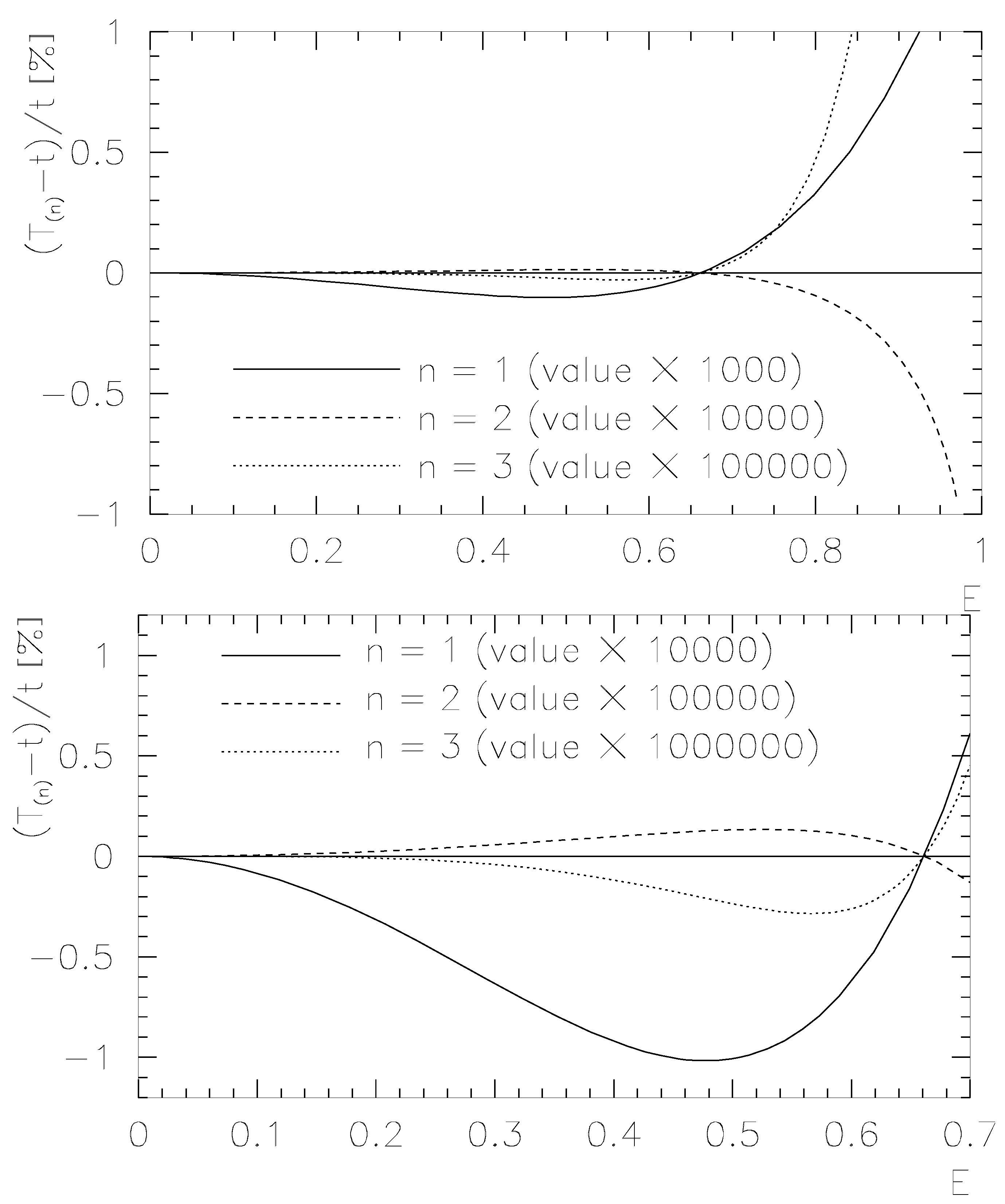
where

D = Δ E_{1} Δ E_{2} Δ E_{3} (Δ E_{1} - Δ E_{2}) (Δ E_{1} - Δ E_{3}) (Δ E_{2} - Δ E_{3})

. For

0 \leq E \leq 0.70

the relative deviation is restricted to

5 \cdot 10^{- 10}

while up to

E = 0.92

the maximal relative deviation is

4 \cdot 10^{- 8}

. The results for the deviations of

T_{(n)}

(

n = 1, 2, 3

) for linear, quadratic and cubic dynamical approximation are shown in Figure 2.

5. Conclusions

In order to test the feasibility and speed, we have coded our algorithm in the computer language C under Slackware 15.0 on an ordinary hp laptop. The dependence of the CPU time for the calculation is estimated by calculating the value

10^{6}

times in sequence. The speed of the calculation of course turns does not depend on the value for E, as the precision is not optimised. This would have to be neccessary for a practical application. For an arbitrary starting value

E = 0.8

we perform this test, and the results are given in Table 1. An analysis of the table shows that a further step in the degree p doubles the run time while the dynamics for increasing n adds a constant value of approximately

0.06

seconds to the result. Despite the fact the increase of the dynamics needs the solution of a linear system of equations and the coding of the result, this endeavour is justified, as by using the dynamics one can increase the precision of the result without loosing calculational speed.

Author Contributions

Conceptualization, D.M.; methodology, D.M. and S.G.; writing—original draft preparation, D.M.; writing—review and editing, S.G. and D.M.; visualization, S.G.; All authors have read and agreed to the published version of the manuscript.

Funding

This research was funded by the European Regional Development Fund under Grant No. TK133.

Institutional Review Board Statement

Not applicable.

Informed Consent Statement

Not applicable.

Data Availability Statement

Not applicable.

Conflicts of Interest

The authors declare no conflict of interest.

References

von Neumann, J.; von Neumann, J. Various Techniques Used in Connection with Random Digits. in Householder, A.S.; Forsythe, G.E.; and Germond, H.H. (eds.). Monte Carlo Methods. National Bureau of Standards Applied Mathematics Series 1951, 12, 36–38. [Google Scholar]
Available online: https://quside.com/quside-unveils-the-worlds-first-randomness-processing-unit.
Craig, J.W. A new, simple and exact result for calculating the probability of error for two-dimensional signal constellations. Proceedings of the 1991 IEEE Military Communication Conference 1991, 2, 571–575. [Google Scholar]
Lever, K.V. New derivation of Craig’s formula for the Gaussian probability function. Electronics Letters 1998, 34, 1821–1822. [Google Scholar] [CrossRef]
Tellambura, C; Annamalai, A. Derivation of Craig’s formula for Gaussian probability function. Electronics Letters 1999, 35, 1424–1425. [CrossRef]
Stewart, S.M. Some alternative derivations of Craig’s formula. The Mathematical Gazette 2017, 101, 268–279. [Google Scholar] [CrossRef]
Martila, D.; Groote, S. Evaluation of the Gauss Integral. Stats 2022, 5, 538–545. [Google Scholar] [CrossRef]
Andrews, L.C. Special functions of mathematics for engineers. SPIE Press 1998, 110. [Google Scholar]
Strecok, A.J. On the Calculation of the Inverse of the Error Function. Math. Comp. 1968, 22, 144–158. [Google Scholar]
Blair, J. M; Edwards, C.A.; Johnson, J.H. Rational Chebyshev Approximations for the Inverse of the Error Function. Math. Comp. 1976, 30, 827–830. [Google Scholar] [CrossRef]
Bergsma, W.P. A new correlation coefficient, its orthogonal decomposition and associated tests of independence. arXiv:math/0604627 [math.ST].
Dominici, D. Asymptotic analysis of the derivatives of the inverse error function. arXiv:math/0607230 [math.CA].
Dominici, D; Knessl, C. Asymptotic analysis of a family of polynomials associated with the inverse error function. arXiv:0811.2243 [math.CA].
Winitzki, S. A handy approximation for the error function and its inverse. Available online: https://www.academia.edu/9730974/.
Giles, M. Approximating the erfinv function. GPU Computing Gems Jade Edition, 2011; 109–116. [Google Scholar]
Soranzo, A; Epure, E. Simply Explicitly Invertible Approximations to 4 Decimals of Error Function and Normal Cumulative Distribution Function. arXiv:1201.1320 [stat.CO].

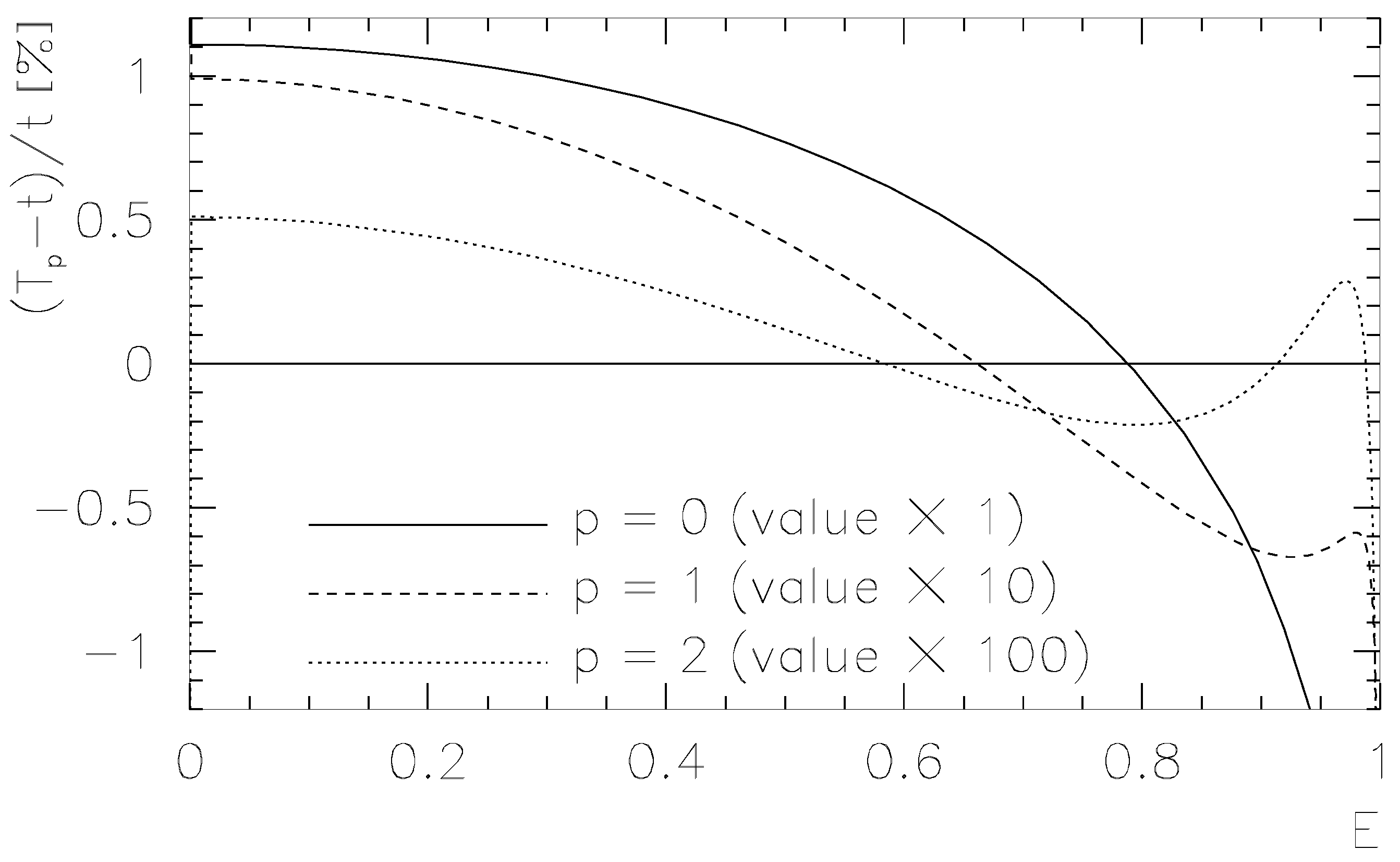
Figure 1. Relative deviations for the statical approximations

Figure 2. Relative deviation for the dynamical approximations (the degree is chosen to be

p = 1

)

Figure 2. Relative deviation for the dynamical approximations (the degree is chosen to be

p = 1

)

Table 1. Run time experiment for our algorithm under C for

E = 0.8

and different values of n and p (CPU time in seconds). As indicated, the errors are in the last displayed digit, i.e.,

\pm 0.01

seconds.

Table 1. Run time experiment for our algorithm under C for

E = 0.8

and different values of n and p (CPU time in seconds). As indicated, the errors are in the last displayed digit, i.e.,

\pm 0.01

seconds.

	$n = 0$	$n = 1$	$n = 2$	$n = 3$
$p = 0$	$0.06 (1)$	$0.12 (1)$	$0.15 (1)$	$0.18 (1)$
$p = 1$	$0.13 (1)$	$0.19 (1)$	$0.22 (1)$	$0.25 (1)$
$p = 2$	$0.24 (1)$	$0.29 (1)$	$0.33 (1)$	$0.36 (1)$

Disclaimer/Publisher’s Note: The statements, opinions and data contained in all publications are solely those of the individual author(s) and contributor(s) and not of MDPI and/or the editor(s). MDPI and/or the editor(s) disclaim responsibility for any injury to people or property resulting from any ideas, methods, instructions or products referred to in the content.

© 2023 by the authors. Licensee MDPI, Basel, Switzerland. This article is an open access article distributed under the terms and conditions of the Creative Commons Attribution (CC BY) license (http://creativecommons.org/licenses/by/4.0/).

Copyright: This open access article is published under a Creative Commons CC BY 4.0 license, which permit the free download, distribution, and reuse, provided that the author and preprint are cited in any reuse.

MDPI Initiatives

Important Links

Choose an area of interest and we will send you notifications of new preprints at your preferred frequency.

Disclaimer

Analytic Error Function and Numeric Inverse Obtained by Geometric Means

Abstract

1. Introduction

2. Derivation of Craig’s integral representation

3. Power series expansion

4. Approximations for the inverse error function

5. Conclusions

Author Contributions

Funding

Institutional Review Board Statement

Informed Consent Statement

Data Availability Statement

Conflicts of Interest

References

MDPI Initiatives

Important Links

Subscribe