1. Introduction
Wheat is one of the most important food crops for humanity, accounting for 21% of the global food demand [
1]. China is the largest wheat-growing country in the world. As one of China’s three major staple crops, winter wheat occupies approximately 22% of the total growing area for food crops and has an important position in grain production, circulation, and consumption. Therefore, timely information on the distribution of winter wheat is of great significance to ensure grain yield [
2]. With the rapid development of remote sensing (RS) and machine learning (ML) technologies, the combination of the two has become an effective means of monitoring the distribution of crops. It takes advantage of not only the macroscopic, economical, and time-sensitive nature of RS technology [
3,
4] but also the automatic image classification capability of ML technology, and therefore, it has become a new research area of intense focus in the field of RS.
Recently, extensive attention has been paid to ML classification methods for crop category extraction based on RS images [
5]. ML algorithms can effectively improve the time efficiency of data processing and the accuracy of classification results through their own heuristic learning strategies and learning engines and therefore have become the mainstream method for RS identification of large areas of crops [
6]. To date, ML methods such as support vector machine (SVM), classification and regression tree (CART), and random forest (RF) have been widely adopted in their respective research fields with good results. Li et al. [
7] used Sentinel-1 RS data to construct a multimodal feature dataset of spectral, textural, and topographic features and used the RF algorithm to effectively extract the winter wheat-growing area at the county scale. Zheng et al. [
8] used multitemporal Landsat normalized difference vegetation index (NDVI) data to effectively classify crops using the SVM algorithm, and Zhao et al. [
9] used the CART algorithm to identify the land use/cover classification of the Jiangning Pilot Area in Jiangsu Province as an example and demonstrated the feasibility of the CART algorithm.
As an ensemble learning algorithm, the extreme gradient boosting (XGBoost) algorithm can adapt to complex nonlinear relationships, and the model has a better parallel processing capability, which can effectively solve the overfitting problem that may occur in ML regression models [
10]. Therefore, it can be used as an effective method for constructing crop identification models in a certain area, thereby promoting the development of hyperspectral RS technology in the field of crop identification [
11]. Zhang et al. [
12] constructed a multisource RS crop identification method based on the XGBoost algorithm by using the time-series spectral and vegetation index features, which can meet the requirements of crop identification applications in cloudy and foggy areas. Based on the XGBoost algorithm, Zhang et al. [
11] established a model for simulating and estimating the meadow aboveground biomass. Xu et al. [
13] used unmanned aerial vehicle RS data and the XGBoost method for mangrove identification based on the fusion features of hyperspectral images and light detection and ranging (LiDAR) point clouds. Deng et al. [
14] used the XGBoost algorithm to classify and extract feature bands of diseased citrus plants based on the full band.
Although the XGBoost algorithm has achieved good results in biomass and forest identification, there are still few studies on the identification of winter wheat, a main food crop in China, based on the XGBoost algorithm. In addition, most of the traditional methods are based on the spectral features of images but have poor identification performance for crops with similar growth periods due to the phenomenon that “the same object shows different spectral characteristics and different objects show the same spectral characteristics.” In [
15] Research has shown that textural features can account for both macroscopic features and microscopic details of crops and have high stability, which can make up for the shortcomings of classification based on image spectral features and can effectively distinguish crop types [
16]. Therefore, using Baoying County in Jiangsu Province, China, as a study area, this paper implemented winter wheat identification based on the XGBoost algorithm under the support of multiple features by using Sentinel-2 data during the main growth period of winter wheat and adopting the spectral, textural, and topographic features of winter wheat in the study area. The XGBoost algorithm-based identification method was compared with traditional identification methods. This paper is expected to provide a guarantee of food security in China and to offer a scientific basis for research on winter wheat growth monitoring and yield estimation.
2. Data and Methods
2.1 Overview of the Study Area
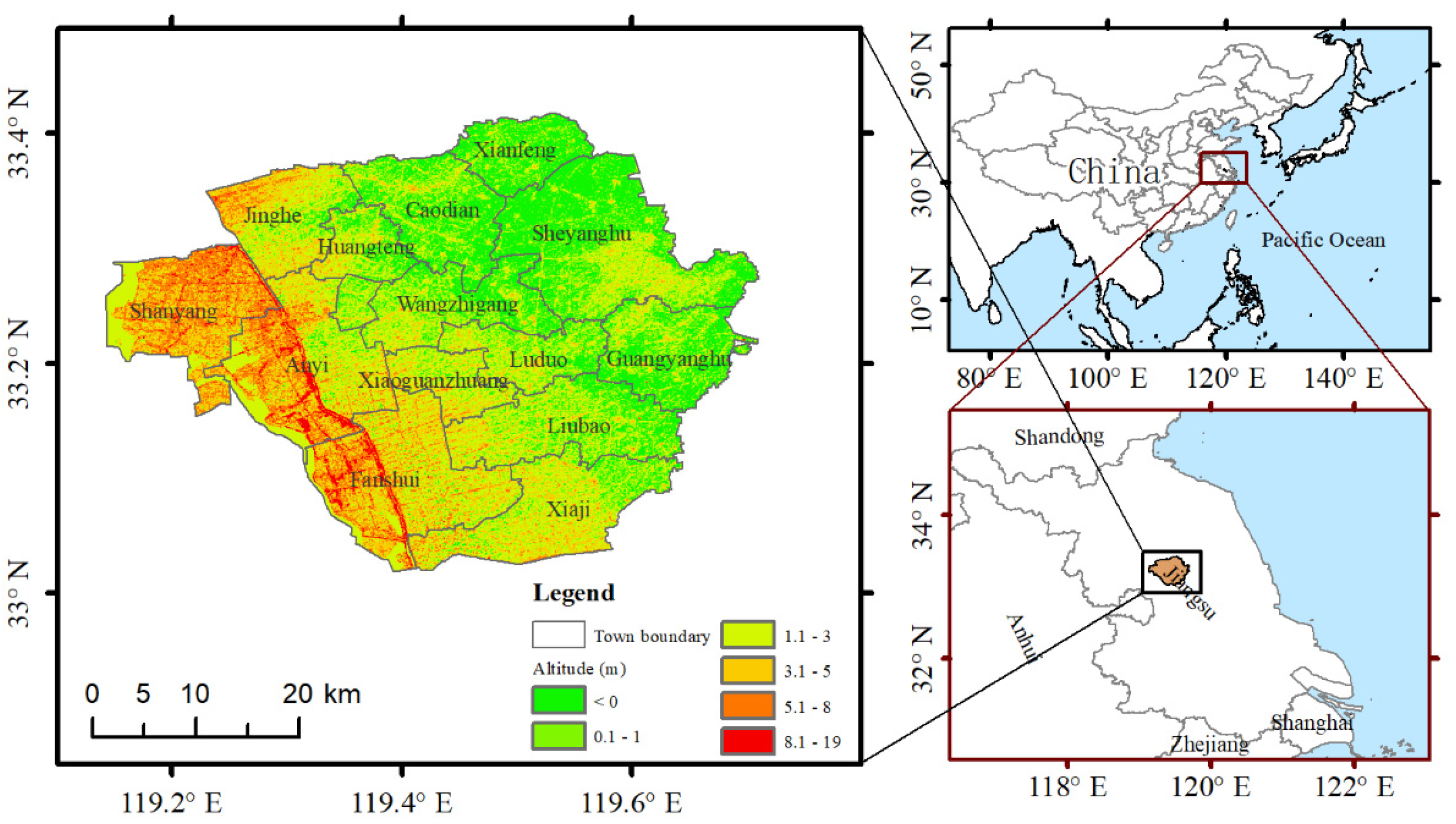
The study area selected in this study was Baoying County, Jiangsu Province, China, located in the central Jiangsu Province, with geographical coordinates of 33°02′–33°24′N and 119°07′–119°42′E (
Figure 1). The fertile soil, vast waters, and mild and humid climate in this area are extremely suitable for the cultivation of winter wheat. The county is rich in agricultural resources, with a crop growing area of 52,800 hectares and winter wheat as the main winter food crop. It is one of the major grain-producing areas for winter wheat in Jiangsu Province. Therefore, this area was selected as a representative study area for winter wheat information extraction.
2.2 RS Data and Preprocessing
Sentinel-2A MultiSpectral Instrument (MSI) data from the main wheat growth period (from January 1, 2022, to June 30, 2022) were used in this paper. Nine RS images with a cloud cover of less than 10% in the study area taken on January 16, February 5, February 25, March 7, April 6, May 6, May 16, June 15, and June 25, 2022, were selected. These data have been processed by radiometric correction, atmospheric correction, and orthorectification, and directly called and processed through the Google Earth Engine (GEE).
GEE is a cloud-based platform for geospatial analysis on a global scale [
17]. Users can not only extract, call, and analyze a vast number of publicly available RS images stored online but also leverage its powerful cloud computing capabilities for online computation and processing. The advent of the GEE platform has greatly improved the efficiency of RS research and provided new opportunities for the rapid classification of RS images, crop extraction, and regional monitoring [
18].
Sentinel-2A MSI data cover a total of 13 spectral bands, with a width of 290 km, ground resolutions of 10, 20, and 60 m, and a revisit period of 10 days, and they have become one of the main data sources for crop classification research [
19].
Shuttle radar topography mission (SRTM) digital elevation data, a type of SRTM data [
20], were obtained jointly by the National Aeronautics and Space Administration, the National Imagery and Mapping Agency (NIMA) of the Department of Defense, and the German and Italian space agencies. The SRTMGL1_003 product used in this paper was provided by the United States Geological Survey at a resolution of 1 arcsecond (~30 m). This paper used this product in the GEE to construct the topographic features, including the elevation and slope, of the study area.
2.3 Sample data
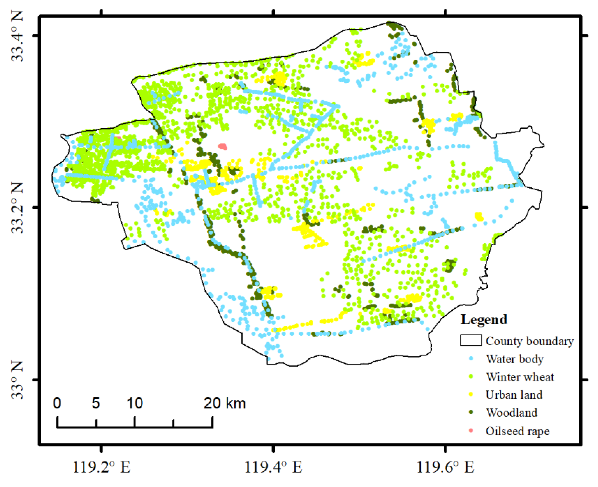
Five typical features, namely, winter wheat, water bodies, urban land, woodland, and oilseed rape, were selected in the study area. Samples were obtained by visual interpretation in addition to field collection. The feature sample points were selected online using the GEE platform and then imported into Google Earth for inspection. After eliminating those with obvious errors, a total of 3651 sample points were obtained, including 1610 samples of winter wheat, 733 samples of water bodies, 634 samples of urban land, 631 samples of woodland, and 43 samples of oilseed rape (
Figure 2). Due to the uneven growing area of traditional agriculture in Baoying County, the proportions of the sown area of food crops [
10] and cash crops (mainly oil crops) are 87.0% and 4.1%, respectively, indicating that food crops dominate while cash crops are small in scale and simple in structure. Therefore, only a small number of oilseed rape samples were selected in this paper to meet the ratio of winter wheat to oilseed rape samples [
21].
2.4 Feature Extraction
Spectral features are important features in current research on crop classification and identification. In this paper, 12 original bands (except the B1 band) were selected from Sentinel-2 RS images for the construction of spectral features, and indices such as the normalized difference vegetation index (NDVI)[
22], enhanced vegetation index (EVI)[
23], normalized difference water index (NDWI)[
24], normalized difference building index (NDBI)[
25], normalized difference tillage index (NDTI)[
26], and modified normalized difference water index (MNDWI)[
27] were used to construct spectral features. As the vegetation indices are mostly constructed based on the red band, chlorophyll absorption is strong in the red band, leading to a decrease in the sensitivity of the vegetation indices to the chlorophyll content; furthermore, the chlorophyll absorption in the red-edge region is lower than that in the red band, effectively reducing the influence of the chlorophyll saturation effect[
28]. In addition, the red-edge is a steeply rising region between the red and near-infrared (NIR) bands, and the spectral features of the red-edge vary between different plant species. Therefore, the classification accuracy can be effectively improved by calculating the vegetation index using the reflectance of the red-edge region[
29], and the red-edge NDVI (RENDVI)[
30] was constructed by using the red-edge band of Sentinel-2 data. A total of 19 spectral features (i.e., 12 original bands plus seven indices) were selected in this paper, namely, B2, B3, B4, B5, B6, B7, B8, B11, and B12, representing blue, green, red, red-edge 1, red-edge 2, red-edge 3, NIR bands, and shortwave bands 1 and 2, respectively; the specific calculation formulas are shown in
Table 1.
This paper also made full use of textural features to improve the classification accuracy of winter wheat-growing areas. The gray-level co-occurrence matrix (GLCM) is a commonly used method for describing texture by studying the spatial correlation characteristics of the gray levels [
31,
32,
33]. Since the NIR band plays an important role in vegetation RS and vegetation reflection is extremely pronounced in the NIR region due to the internal structure of the leaves, Sentinel-2 data in the NIR band (B8) were used to calculate the textural features [
34]. The GLCM textural feature function in the GEE was called to calculate six textural features [
35,
36]: variance (B8_var), contrast (B8_contrast), entropy (B8_ent), correlation (B8_corr), angular second-order distance (B8_asm), and inverse difference moment (B8_idm). In addition, two topographic features, elevation and slope, were constructed by calling the SRTMGL_003 data in the GEE. A total of 27 features are used in this paper, see
Table 2 for details.
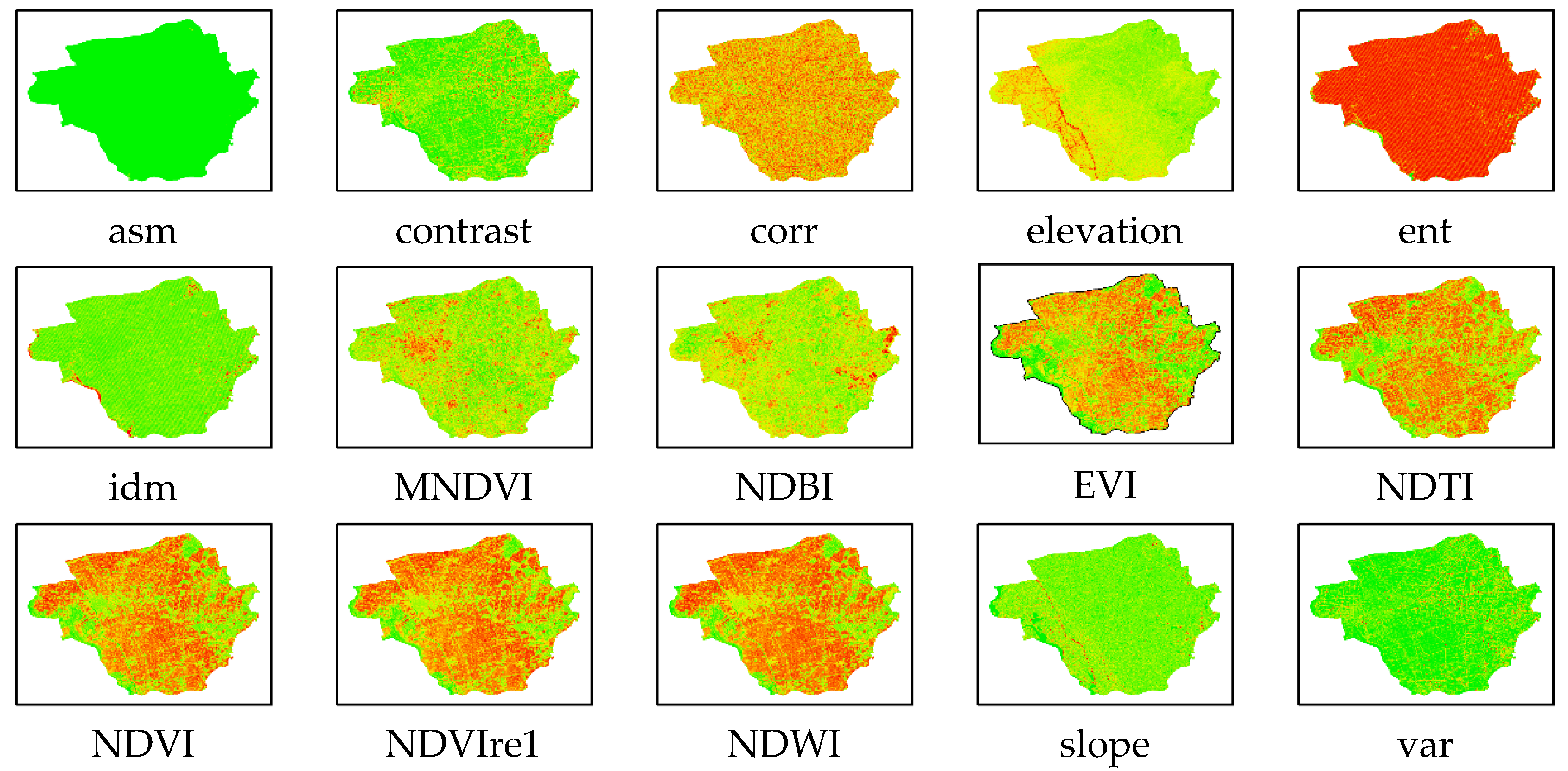
Finally, a median composite of all Sentinel-2 images from this growth period was computed to obtain a synthesized spectral, textural, and topographic feature image with 27 bands with a spatial resolution of 10 m [
37]. The composite image of the main features is shown in
Figure 3.
2.5 XGBoost Algorithm
Proposed by Chen et al. [
38], the XGBoost algorithm was developed by optimizing the gradient boosting (GDBT) algorithm. Compared with GDBT, XGBoost is characterized by high accuracy, less overfitting, and strong scalability [
39]. Its core is to integrate multiple weak learners into a strong learner through a certain method using the GDBT algorithm. First, a weak learner is trained using the initial training set, and then, the weights of the training samples in the next weak learner are optimized according to the performance of the previous weak learner until the Kth weak learner is optimized. Finally, the weighted combination of the trained multiple learners is used as the final prediction result [
12].
where
is the feature of the ith sample,
is the prediction of the kth weak learner, and
is the model’s prediction.
The objective function of XGBoost (Equation (2)) consists of two parts: the loss function, which measures the training error, and the regularization term, which controls the complexity.
In Equations (2) and (3), is the loss function, which is used to measure the error between the true value and the model prediction . The default loss function used in this classification model is the root mean squared error (RMSE), and Ω is the regularization term, which is used to control the model complexity to prevent it from overfitting. represents the complexity of the kth weak learner, and c is a constant term.
The loss function is expanded by the Taylor series to obtain the approximate objective function, and the constant term c can be ignored.
where
and
denote the first and second derivatives of the loss function
, respectively.
The complexity of the model depends on many factors. In the XGBoost classification model, it is mainly determined by the number of leaf nodes and the smoothness of the corresponding node weights.
where γ and λ are both manually set parameters, T is the number of leaf nodes, ω is the weight of each leaf, and
is the regularization penalty term for the weight parameter ω.
The combination of Equations (4) and (5) results in Equation (8) for the optimal leaf node weight and Equation (9) for the algorithm’s optimal objective function.
where
and
; In the above equations,
is a fixed coefficient,
is the complexity parameter,
is the number of leaf nodes in the tree,
is the cumulative sum of the first partial derivatives
of the samples contained in leaf node j, and
is the cumulative sum of the second partial derivatives
of the samples contained in leaf node j.
2.6 Traditional ML Algorithms
Three representative traditional ML algorithms, namely, RF, SVM, and CART, were selected in this paper for comparison with the XGBoost algorithm.
Proposed by Breiman [
40], an American scientist, RF is a classification algorithm that can efficiently process datasets with multidimensional features and seek the optimal solution for category attribution through cross-validation of sample features. It has the advantages of a fast training speed, insensitivity to sample size, high classification accuracy, and strong antinoise ability, making it an ML algorithm that is widely used for intelligent learning of agricultural RS big data [
41]. In this paper, an RF model was built using the ee.Classifier.smileRandomForest function in the GEE platform with the number of decision trees set to 100 and all other parameters set to their default values.
The SVM is an ML algorithm based on the statistical learning theory developed by the Vapnik team [
42]. It is one of the most novel and practical methods in statistical learning theory. The SVM is characterized by the ability to minimize empirical error and maximize the classification interval at the same time, i.e., it achieves supervised learning by finding a hyperplane that both guarantees classification accuracy and maximizes the interval between the two types of data. This method has a strong ability to process nonlinear and high-dimensional data and also solves the curse of dimensionality problem, making it a current research area of major focus in the international ML community [
43]. In this paper, an SVM model was built using the ee.Classifier.libsvm function in the GEE platform with all parameters set to their default values.
CART is a decision tree construction algorithm proposed by Breiman [
44] in 1984, and it has been improved continuously. Its basic principle is the creation of a decision tree structure in the form of a binary tree by cyclic bisection of the training dataset, which is composed of test and target variables. The algorithm can be used for both classification and prediction of continuous variables. It is structurally clear, easy to understand, simple to implement, fast and accurate, and can handle both a large amount of data and high-dimensional data effectively. In addition, it does not require any statistical distribution of the input data, which can be continuous or discrete. The CART algorithm can also determine the importance of test variables [
9]. In this paper, a decision tree model was built using the ee.Classifier.smileCart function in the GEE platform with the parameter set to 100 and the rest of the parameters set to default values.
2.7 Accuracy Evaluation
The use of a confusion matrix is a standard method for evaluating the accuracy of RS image classification results [
45]. The confusion matrix, also known as the error matrix, is represented as a matrix with n rows and n columns (
Table 3).
This paper selected four accuracy evaluation indicators, namely, user accuracy (UA), producer accuracy (PA), overall accuracy (OA), and the kappa coefficient to evaluate the accuracy of three classifiers for winter wheat identification.
In Equations (8)–(11), represents the positive samples correctly classified by the model, with both predicted and true values being 1; represents the positive samples misclassified by the model, with the predicted and real values being 1 and 0, respectively; denotes the negative samples correctly classified by the model, with both predicted and true values being 0; represents the negative samples misclassified by the model, with the predicted and true values being 0 and 1, respectively; is the sum of the number of correctly classified samples in each category divided by the total number of samples, i.e., the overall classification accuracy; and is the sum of the product of the true and predicted numbers of samples in each category divided by the square of the total number of samples.
3. Materials and Methods
3.1 Classification Model Training
The XGBoost model was built using Python 3.9. A sample dataset containing 27 feature bands was exported as training samples. A total of 70% of the samples were randomly selected to train the XGBoost model to classify the features in the study area, and the remaining 30% of the samples were used as test samples to evaluate the accuracy of the crop identification results. In addition, to improve the model’s identification accuracy, the parameters needed to be reasonably adjusted before building the model. The number of weak learners in the model is the primary parameter that affects the final model’s accuracy. A larger number of weak learners is not always better, as too many weak learners can lead to model overfitting and increased computational burden.
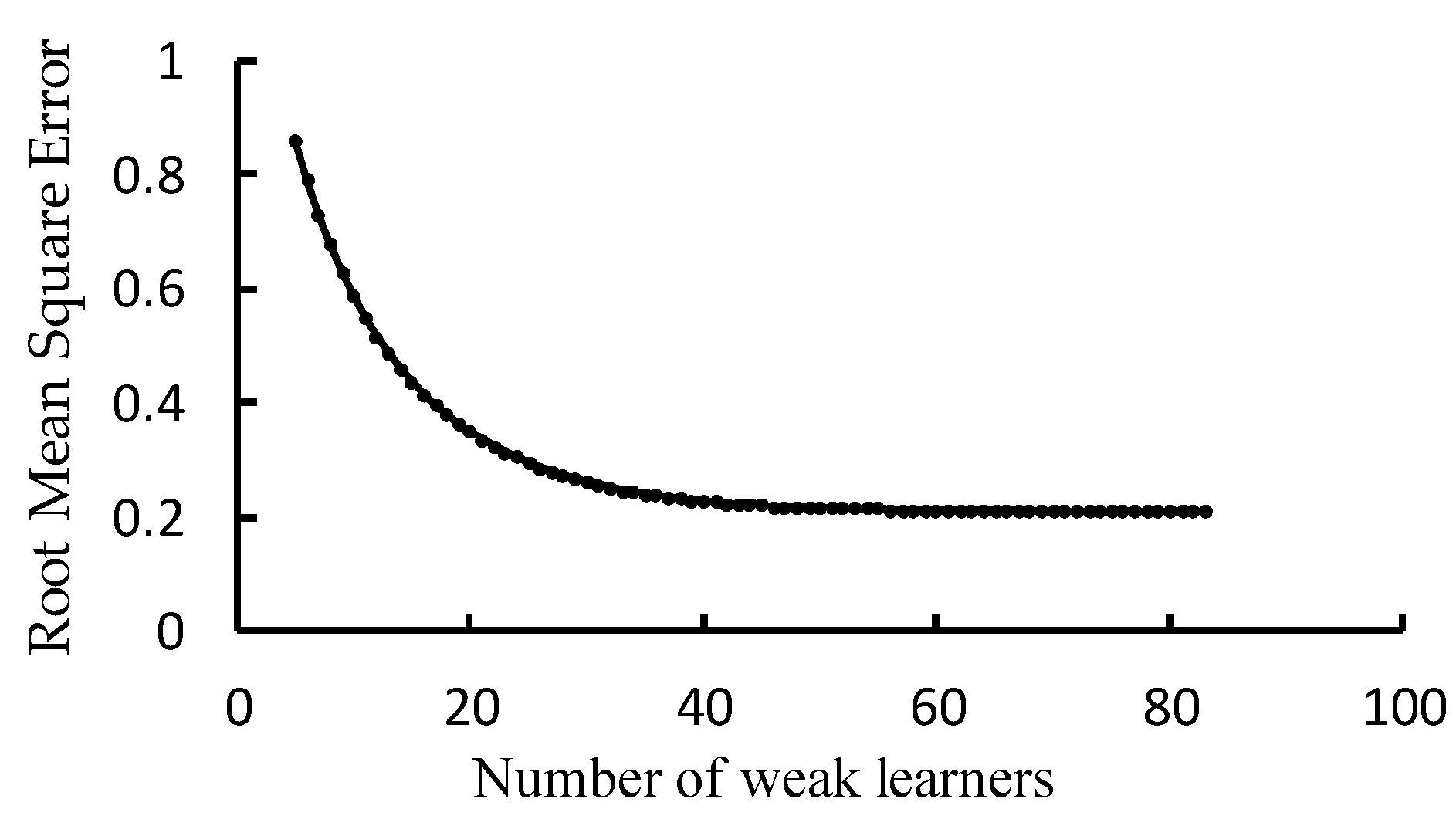
The learning curve in
Figure 4 demonstrates that the average absolute error dropped sharply as the number of weak learners increased from 0 to 30 and then gradually became stable, reaching the lowest average absolute error with 75 weak learners, and the program stopped early at 83 runs. Therefore, 75 weak learners were used as the optimal number for this training sample set. The other parameters were optimized by the learning curve and the grid search methods, including key parameters such as the step size (learning_rate), the maximum tree depth (max_depth), the minimum leaf weight (min_child_weight), and the minimum loss function drop (gamma) for each training set. The specific optimal parameters are as follows: learning_rate/step = 0.1, number of weak learners = 75, max_depth = 6, min_child_weight = 1; the rest of the parameters were set to default values.
3.2 XGBoost Classification Results
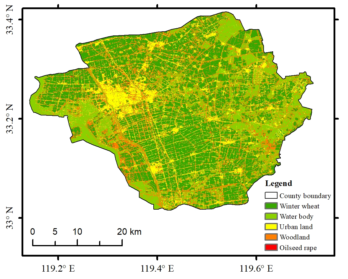
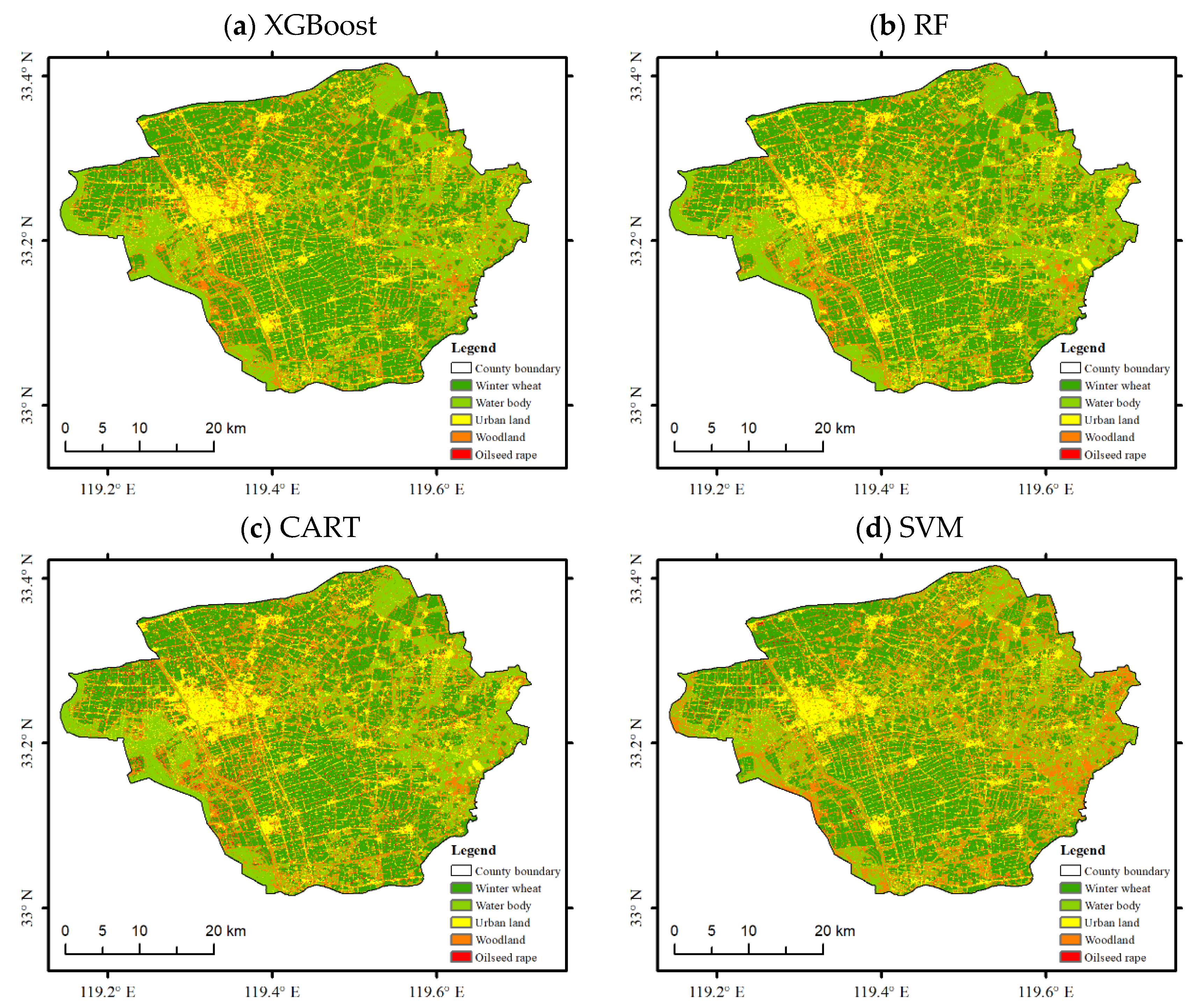
Figure 5a shows the spatial distribution of winter wheat based on the XGBoost algorithm model.
Table 4 presents the results of the accuracy evaluation for the winter wheat identification results based on the four algorithms.
Figure 5a and
Table 4 indicate that the use of the XGBoost algorithm to identify the winter wheat-growing area in Baoying County with the same sample set finally led to an overall identification accuracy of 93.43%, a winter wheat producer accuracy of 98.01%, a consumer accuracy of 93.53%, and a kappa coefficient of 0.9059, which essentially met the accuracy requirements for crop identification in the study area.
To objectively evaluate the extraction performance of the XGBoost classification model on winter wheat in the study area, this paper used the measured sample points except for the training set and the test set, combined with the mixed sample points selected by visual interpretation, for comparison with the extraction results by the model. It was found through comparison with the information for the sample points that the winter wheat in each township could essentially be correctly extracted, and thus, the extraction results were satisfactory. Only a small amount of misclassification occurred in Sheyanghu Town and Guangyanghu Town. Because field investigation revealed that fishponds, winter wheat, and oilseed rape were scattered in these areas, the misclassification and missed classification might be attributed to the phenomenon that different objects can show the same spectral characteristics. Overall, this paper had a low misclassification rate and a missed classification rate, and the winter wheat extraction model had a high identification accuracy, thereby successfully identifying winter wheat in the study area.
3.3 Comparison with the Classification Results of Traditional ML Algorithms
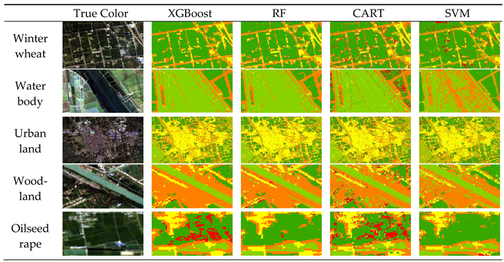
The winter wheat identification and classification results of the three traditional ML algorithms, namely, RF, SVM, and CART, were compared with those of the XGBoost algorithm in
Figure 5.
Table 5 is a comparison of typical feature extraction results based on four types of machine learning. Evidently, the classification results based on the XGBoost algorithm were significantly better than the other three classification results and effectively distinguished winter wheat from other features.
As shown in
Table 4, the overall accuracies of the XGBoost, RF, CART, and SVM algorithms were 93.43%, 93.25%, 89.75%, and 89.15%, respectively, with XGBoost having the highest overall accuracy, which was slightly higher than RF and significantly higher than CART and SVM. The kappa coefficient of the XGBoost classification results was also the highest. The four algorithms were sorted in descending kappa coefficient order as XGBoost, RF, CART, and SVM, with the kappa coefficient of XGBoost having the highest accuracy of 0.9059. The four algorithms were sorted in descending order according to the producer accuracy of winter wheat as XGBoost, RF, SVM, and CART, which were 98.01%, 96.49%, 93.53%, and 92.79%, respectively. The CART algorithm had the highest customer accuracy for winter wheat, which was 96.17%.
The official statistical area of winter wheat in Baoying County was searched in terms of the grain sown area and yield data in the 2022 Yangzhou Statistical Yearbook released by the Yangzhou Bureau of Statistics. The winter wheat-growing area was found to be 53,462.67 hectares in 2021. Using the official statistical area published as the benchmark, the area accuracy of each model result was evaluated, and the results are shown in
Table 6. The area extracted by XGBoost and RF was closer to the official statistical value, while the area of winter wheat extracted by CART and the SVM had a large error compared with the official statistical value. Among them, the area extracted by the XGBoost method had the highest accuracy, which was only 5.64% less than the official statistic data, demonstrating relatively good performance.
4. Discussion
In this paper, good results were achieved in terms of identifying winter wheat based on the XGBoost algorithm. The overall accuracy was improved to some extent compared with that in the paper by Zhang et al. [
12] by using the XGBoost algorithm to identify crops in cloudy and foggy areas. This improved accuracy is a result of the textural features added in this paper to the feature bands in the training samples to improve the classification accuracy for winter wheat-growing areas. As important structural information about the spatial distribution of features, textural features compensate for the deficiency of spectral features in the classification of hyperspectral RS images to a certain extent and partially offset the influence of clouds and fog [
46,
47]; thus, the identification accuracy was higher than that of the results from Zhang et al. Using the textural features of Satellite pour l’Observation de la Terre (SPOT5) images, Li et al. [
48]estimated and verified the biomass of each of five forest types and found that the textural features contributed significantly to the model, demonstrating the importance of textural features in model construction. In their parametric study of a tropical rainforest stand using Landsat images, Lu et al. [
49] found that the accuracy of forest biomass estimation was higher when textural features were combined with spectral features than when band values or vegetation indices were used alone, further confirming this point.
Sample selection is also an important factor that affects the identification accuracy. Both the type and number of samples affect the model accuracy to a certain extent. This paper only selected five typical features in the study area, and an appropriate increase in the size of the sample data set can improve the identification accuracy. However, it is not necessarily the case that more feature variables in the model lead to better results; instead, too many features can easily cause data redundancy and overfitting of the identification results. In addition, because this study area clearly presents plain landforms, it is questionable to include topographic features in the feature variables. Therefore, the selection of appropriate feature variables during model construction also played a crucial role in the identification of winter wheat in the study area.
5. Conclusion
Using winter wheat in Baoying County in Jiangsu Province, China, as a research object, this paper used Sentinel-2 images as the data source to construct spectral, textural, and topographic features, used the XGBoost algorithm to identify and extract winter wheat during the growth period, and compared the results with those of traditional ML algorithms. The following conclusions are drawn:
(1) Using Sentinel-2 data in the main growth period of crops in Baoying County, a sample training set and a validation set containing 27 features were constructed by considering nineteen spectral features, six texture features, and two topographic features. A model based on the XGBoost algorithm was constructed using Python, the model parameters were optimized, the standard sample model was trained, and the crop identification model for the classification and extraction of winter wheat was constructed.
(2) In the identification of winter wheat in the study area, the XGBoost algorithm had the highest overall accuracy (93.43%) and the largest kappa coefficient (0.9059), and its result had only a small error compared with the actual winter wheat-growing area in Baoying County, essentially meeting the accuracy requirement for crop identification in the study area.
(3) The algorithm XGBoost far outperformed the three traditional ML algorithms. Among the traditional ML algorithms, only the RF algorithm had good accuracy, with an overall accuracy only slightly lower than that of the XGBoost algorithm, while the SVM and CART algorithms had low accuracy, and their results had a large error compared with the actual winter wheat-growing area in Baoying County.
This paper showed that the XGBoost algorithm demonstrates good performance in fast and accurate estimation of the winter wheat-growing area, which is of great significance in terms of estimating yield and ensuring food security. In future research, the XGBoost-based crop identification model can be further optimized to provide a better experience and more technical methods for winter wheat identification.
Author Contributions
Conceptualization, Y.W. and Y.D.; methodology, Y.W.; software, D.Z.; validation, Y.W. and Y.D.; writing—original draft preparation, Y.W.; writing—review and editing, D.Z.; visualization, Y.D. All authors have read and agreed to the published version of the manuscript.
Funding
This research was funded by National Key R&D Program of China, grant number 2019YFB2102003.
Institutional Review Board Statement
Not applicable.
Data Availability Statement
The data presented in this study are available on request from the corresponding author. The data are not publicly available due to institutional policy.
Acknowledgments
We thank to the reviewers for the constructive and valuable comments and the editors for their assistance in refining this paper.
Conflicts of Interest
The authors declare no conflict of interest.
References
- Atamanyuk, I.; Havrysh, V.; Nitsenko, V.; et al. Forecasting of Winter Wheat Yield: A Mathematical Model and Field Experiments. Agriculture 2023, 13, 41. [Google Scholar] [CrossRef]
- Zhao, G.; Chang, X.; Wang, D.; et al. Research Report on Development of China’s Wheat Production Potential. Crops 2012, 148, 1–5. [Google Scholar]
- Zwart, S.J.; Bastiaanssen, W.G.M.; de Fraiture, C.; et al. WATPRO: A remote sensing based model for mapping water productivity of wheat. Agric. Water Manag. 2010, 97, 1628–1636. [Google Scholar] [CrossRef]
- Zhang, H.; Du, H.; Zhang, C.; et al. An automated early-season method to map winter wheat using time-series Sentinel-2 data: A case study of Shandong, China. Comput. Electron. Agric. 2021, 182, 105962. [Google Scholar] [CrossRef]
- Wang, Z. Exponential stability of numerical solutions to stochastic forest evolution system. J. Southwest Minzu Univ. (Nat. Sci. Ed.) 2017, 43, 623–629. [Google Scholar]
- Liang, J.; Zheng, Z.; Xia, S.; et al. Crop recognition and evaluationusing red edge features of GF-6 satellite. Natl. Remote Sens. Bull. 2020, 24, 1168–1179. [Google Scholar] [CrossRef]
- Li, C.; Chen, W.; Wang, Y.; et al. Extraction of Winter Wheat Planting Area in County Based on Multi-sensor Sentinel Data. Trans. Chin. Soc. Agric. Mach. 2021, 52, 207–215. [Google Scholar]
- Zheng, B.; Myint, S.W.; Thenkabail, P.S.; et al. A support vector machine to identify irrigated crop types using time-series Landsat NDVI data. Int. J. Appl. Earth Obs. Geoinf. 2015, 34, 103–112. [Google Scholar] [CrossRef]
- Zhao, P.; Fu, Y.; Zheng, L.; et al. Cart-based Land Use/cover Classification of Remote Sensing Images. Natl. Remote Sens. Bull. 2005, 708–716. [Google Scholar]
- Samat, A.; Li, E.; Wang, W.; et al. Meta-XGBoost for hyperspectral image classification using extended MSER-guided morphological profiles. Remote Sens. 2020, 12, 1973. [Google Scholar] [CrossRef]
- Zhang, Y.; Liu, T.; Tong, X.; et al. Hyperspectral remote sensing inversion of meadow aboveground biomass based on an XGBoost algorithm. Acta Prataculturae Sin. 2021, 30, 1–12. [Google Scholar] [CrossRef]
- Zhang, C.; Chen, C.; Xu, H.; et al. Multi-source Remote Sensing Crop ldentification Based on XGBoost Algorithm in Cloudy and Foggy Area. Trans. Chin. Soc. Agric. Mach. 2022, 53, 149–156. [Google Scholar]
- Xu, Y.; Zhen, J.; Jiang, X.; et al. Mangrove species classification with UAV-based remote sensing data and XGBoost. Natl. Remote Sens. Bull. 2021, 25, 737–752. [Google Scholar] [CrossRef]
- Deng, X.; Zeng, G.; Zhu, Z.; et al. Classification and feature band extraction of diseased citrus plants based on UAV hyperspectral remote sensing. J. South China Agric. Univ. 2020, 41, 100–108. [Google Scholar] [CrossRef]
- Man, W.; Li, C. Study on the land use dynamic changes by the RS and GIS of Yan-Long-Tu area. Agric. Sci. J. Yanbian Univ. 2012, 34, 21–26. [Google Scholar]
- Zhang, M. The Role of Texture Features in Hyperspectral Remote Sensing Images. Eng. Technol. Res. 2022, 7, 219–221. [Google Scholar]
- Gorelick, N.; Hancher, M.; Dixon, M.; et al. Google Earth Engine: Planetary-scale geospatial analysis for everyone. Remote Sens. Environ. 2017, 202, 18–27. [Google Scholar] [CrossRef]
- Zhang, W.; Brandt, M.; Wang, Q.; et al. From woody cover to woody canopies: How Sentinel-1 and Sentinel-2 data advance the mapping of woody plants in savannas. Remote Sens. Environ. 2019, 234, 111465. [Google Scholar] [CrossRef]
- Guo, J.; Zhu, L.; Jin, B. Crop Classification Based on Data Fusion of Sentinel-1 and Sentinel-2. Trans. Chin. Soc. Agric. Mach. 2018, 49, 192–198. [Google Scholar]
- Wang, Y.; Qi, Q.; Liu, Y. Unsupervised segmentation evaluation using area-weighted variance and Jeffries-Matusita distance for remote sensing images. Remote Sens. 2018, 10, 1193. [Google Scholar] [CrossRef]
- Wu, B. The supply-side structural reform of agricultural industry in Baoying County. Rural Econ. Sci. -Technol. 2017, 28, 127–128. [Google Scholar]
- Tucker, C.J. Red and photographic infrared linear combinations for monitoring vegetation. Remote Sens. Environ. 1979, 8, 127–150. [Google Scholar] [CrossRef]
- Huete, A.R.; Liu, H.Q.; Batchily, K.V.; et al. A comparison of vegetation indices over a global set of TM images for EOS-MODIS. Remote Sens. Environ. 1997, 59, 440–451. [Google Scholar] [CrossRef]
- McFeeters, S.K. The use of the Normalized Difference Water Index (NDWI) in the delineation of open water features. Int. J. Remote Sens. 1996, 17, 1425–1432. [Google Scholar] [CrossRef]
- Zha, Y.; Gao, J.; Ni, S. Use of normalized difference built-up index in automatically mapping urban areas from TM imagery. Int. J. Remote Sens. 2003, 24, 583–594. [Google Scholar] [CrossRef]
- Serbin, G.; Daughtry, C.S.T.; Hunt, E.R., Jr.; et al. Effect of soil spectral properties on remote sensing of crop residue cover. Soil Sci. Soc. Am. J. 2009, 73, 1545–1558. [Google Scholar] [CrossRef]
- Xu, H. Modification of normalised difference water index (NDWI) to enhance open water features in remotely sensed imagery. Int. J. Remote Sens. 2006, 27, 3025–3033. [Google Scholar] [CrossRef]
- Pu, Y.; Zhang, D.; Xu, D.; et al. Evaluation of Red Edge of Sentinel-2A in Vegetation Classification of Lakeside Zone. For. Resour. Manag. 2021, 131–139. [Google Scholar] [CrossRef]
- Vincent, A.; Kumar, A.; Upadhyay, P. Effect of red-edge region in fuzzy classification: A case study of sunflower crop. J. Indian Soc. Remote Sens. 2020, 48, 645–657. [Google Scholar] [CrossRef]
- You, N.; Dong, J.; Huang, J.; et al. The 10-m crop type maps in Northeast China during 2017–2019. Sci. Data 2021, 8, 41. [Google Scholar] [CrossRef]
- Haralick, R.M.; Shanmugam, K.; Dinstein, I.H. Textural features for image classification. IEEE Trans. Syst. Man Cybern. 1973, 610–621. [Google Scholar] [CrossRef]
- Zhang, B. Texture feature extraction analysis of remote sensing image based on gray level co-occurrence matrix. City Geogr. 2017, 190. [Google Scholar]
- Lin, X.; Peng, D.; Huang, G.; et al. Object-oriented classification with multi-scale texture feature based on remote sensing image. Eng. Surv. Mapp. 2016, 25, 22–27. [Google Scholar]
- He, Z.X.; Zhang, M.; Wu, B.F.; et al. Extraction of summer crop in Jiangsu based on Google Earth Engine. J. Geo-Inf. Sci. 2019, 21, 752–766. [Google Scholar]
- Feng, J.; Yang, Y. Study of texture images extraction based on gray level co-occurrence matrix. Beijing Surveying and Mapping 2007, 84, 19–22. [Google Scholar]
- Jiao, P.; Guo, Y.; Liu, L.; et al. Implementation of gray level co-occurrence matrix texture feature extraction using matlab. Comput. Technol. Dev. 2012, 22, 169–171. [Google Scholar]
- Liu, S.; Peng, D.; Zhang, B.; et al. The Accuracy of Winter Wheat Identification at Different Growth Stages Using Remote Sensing. Remote Sens. 2022, 14, 893. [Google Scholar] [CrossRef]
- Chen, T.; Guestrin, C. Xgboost: A scalable tree boosting system. In Proceedings of the 22nd ACM SIGKDD international conference on knowledge discovery and data mining, 2016.
- Cai, L.; Wu, D.; Fang, L.; et al. Tree Species ldentification Using XGBoost Based on GF-2 Images. For. Resour. Manag. 2019, 44–51. [Google Scholar] [CrossRef]
- Breiman, L. Random forests. Mach. Learn. 2001, 45, 5–32. [Google Scholar] [CrossRef]
- Fang, K.; Wu, J.; Zhu, J.; et al. A Review of Technologies on Random Forests. J. Stat. Inf. 2011, 26, 32–38. [Google Scholar]
- Vapnik, V. The nature of statistical learning theory; Springer science & business media, 1999.
- Du, P.; Lin, H.; Sun, D. On Progress of Support Vector Machine Based Hyperspectral RS Classification. Bull. Surv. Mapp. 2006, 37–40+50. [Google Scholar]
- Breiman, L.; Friedman, J.; Olshen, R.; et al. Cart. Classification and regression trees, 1984.
- Congalton, R.G.; Green, K. Assessing the accuracy of remotely sensed data: Principles and practices; CRC Press: 2019.
- Zhao, S.; An, R. Hyperspectral Remote Sensing Image Recognition Based on Feature Mining. J. Subtrop. Resour. Environ. 2019, 14, 87–94. [Google Scholar]
- Shao, W.; Sun, W.; Yang, G. Comparison of Texture Feature Extraction Methods for Hyperspectral Imagery Classification. Remote Sens. Technol. Appl. 2021, 36, 431–440. [Google Scholar]
- Li, M.; Tan, Y.; Pan, J.; et al. Modeling forest aboveground biomass by combining spectrum, textures and topographic features. Front. For. China 2008, 3, 10–15. [Google Scholar] [CrossRef]
- Lu, D.; Mausel, P.; Brondızio, E.; et al. Relationships between forest stand parameters and Landsat TM spectral responses in the Brazilian Amazon Basin. For. Ecol. Manag. 2004, 198, 149–167. [Google Scholar] [CrossRef]
|
Disclaimer/Publisher’s Note: The statements, opinions and data contained in all publications are solely those of the individual author(s) and contributor(s) and not of MDPI and/or the editor(s). MDPI and/or the editor(s) disclaim responsibility for any injury to people or property resulting from any ideas, methods, instructions or products referred to in the content. |
© 2023 by the authors. Licensee MDPI, Basel, Switzerland. This article is an open access article distributed under the terms and conditions of the Creative Commons Attribution (CC BY) license (http://creativecommons.org/licenses/by/4.0/).
