Modelling and Stability Analysis of the Dynamics of Measles with Application to Ethiopian Data

Preprint

Article

Modelling and Stability Analysis of the Dynamics of Measles with Application to Ethiopian Data

Altmetrics

Downloads

299

Views

182

Comments

A peer-reviewed article of this preprint also exists.

Submitted:

22 March 2023

Posted:

23 March 2023

You are already at the latest version

Alerts

Abstract

Measles is a highly contagious airborne disease that is endemic in many developing countries with low levels of vaccination coverage. In this paper, we propose a deterministic compartmental mathematical model for measles disease dynamics. We establish the global stability conditions for the disease-free and endemic equilibria using the Lyapunov function stability method. \textcolor{red}{Using arbitrary parameters it is obtained that the proposed model exhibits forward bifurcation}. Numerical integration using MATLAB software was used to simulate the model solution of the forward problem. We calibrate the proposed model to estimate the parameters with a 95\% confidence interval (CI) using real data from Ethiopia by formulating an inverse problem. We notice that the model fits well with the real data of Ethiopia. The estimated basic reproduction number ($R_0$) is found to be $R_0=1.3973$ which proves that the disease is endemic. It is also obtained from the local sensitivity analysis that reducing the transmission rate and increasing the vaccination rate could effectively minimize the $R_0$.

Keywords:

Subject: Medicine and Pharmacology - Medicine and Pharmacology

1. Introduction

Measles is an acute viral illness caused by the pathogen

Morbillivirus

whose only reservoir is the human host. Despite an extensive vaccination against measles, it is still endemic in many countries and is the main cause of morbidity and mortality in developing regions [1,2]. Clinical symptoms of measles include: cough, runny nose, red eyes, sore throat, fever and a widespread skin rash. If the virus is transmitted to the susceptible ones, they become exposed and pass the latent period within the first 6 to 9 days of exposure, after that the infectious period follows and are able to transmit the disease for 6 to 7 days [3,4]. An individual once infected with measles becomes lifelong immune after running its entire course.

Mathematical modelling has been broadly used as a tool to understand the mechanisms by which infectious diseases spread, to decide on how to control the spread and to minimize expenses in controlling disease outbreaks [5,6,7,8,9]. The predictive nature of these epidemic models which aids in decision making is one of the key strengths of such models. One of the challenges in epidemic modelling is the analyses of the global stability of the disease-free and endemic equilibria. So far, the most powerful method for global stability analyses of infectious diseases is the direct Lyapunov and the geometric methods [10,11,12,13,14]. The authors [10,11] studied the global stability analyses of

S I S

S I R

, and

S I R S

epidemic models with constant recruitment, disease-induced death and standard incidence rate using Lyapunov functions. However, constructing a Lyapunov function to establish the global stability of an

S E I R

system with constant recruitment, standard incidence, and disease-induced death is still difficult. Moreover, an epidemic model must be validated to check if it is to be actually used [7,15,16,17], which contains comparing the real data with the model solutions in order to evaluate if the model proposed correspond to reality. In most cases, the first model solutions fail to agree with the observed real data, probably due to wrong choice of the initial parameters and lack of adequate model assumptions. Even though, the first model solutions fail to agree with the observed real data, it can be adjusted through a process known as model calibration. Model calibration is the process whereby parameter values that promote a good agreement between the model solutions and observed real data are estimated.

Quite recently, studying the dynamics of the measles disease in the context of mathematics is an important issue [4,18,19,20,21,22,23]. Some authors such as [20,22,23] have studied the dynamics using constant and continuous controls. They have studied the global stability analyses of the disease-free and endemic equilibria. Other authors, for instance, [19] investigated the global stability analysis of the disease dynamics but failed to predict the disease dynamics in the context of a particular situation. There are also others such as [21] who proposed a mathematical model of measles and predicted the disease situation in Bangladesh using double vaccination doses. However, the majority of previous works failed to assume standard incidence in the rate of disease transmission and include disease-induced death rate in the study of the dynamics of the disease. Moreover, few researchers have addressed the estimation of the parameters of the proposed model using real data. Therefore, it is important to study the global dynamics of the measles model by assuming the standard incidence in the disease transmission and estimating the parameters of the proposed model to predict the future situation of a particular region.

This work aims to propose a deterministic compartmental mathematical model for the dynamics of measles disease and calibrate the model to real data of measles outbreaks in Ethiopia. Particularly, we study the long-term global stability analyses of the disease-free and endemic equilibria using the Lyapunov stability method. We also investigate the bifurcation analysis. Next, the model is extended by assuming a fraction of the individuals recruited due to birth or immigration are vaccinated and then model predictions are done to compare model solutions and the real data using some plausible parameters as initial values. Then, a rigorous process of model calibration is done through the solution of an inverse problem to find the best parameter estimates. Finally, the local sensitivity analysis of the basic reproduction number to the estimated parameter values is done to check the robustness of the system proposed.

The work has seven sections: The measles model is formulated in Section 2. In Section 3, we study the mathematical analysis: The basic reproduction number, existence of equilibria, the local and global stability analysis of the equilibria and following this the bifurcation analysis is done in Section 4. The system parameters are estimated in Section 5. In Section 6, numerical simulation of the system is performed. Finally, we conclude the work in Section 7.

2. Mathematical Model Formulation

To formulate the mathematical model of measles, the population is divided into four mutually exclusive classes with each class representing the health condition of an individual. Susceptible individuals (S), individuals carrying the pathogen transmitting the disease but show no clinical symptoms of measles (E), individuals infected with measles, showing the symptoms and can spread the disease (I). Finally, the recovered from measles (R), members who are not infected. The total human population is denoted by

N = S + E + I + R

Some of the main assumptions made in the formulation of the deterministic system (1) are: The population is homogeneously mixed. All susceptible individuals have the same probability of being infected. The incidence is assumed to be standard incidence from the assumption that the rate of contact is constant. An individual infected of measles will either die or recover. There exist life long immunity for the measles disease survivors and hence the model proposed is a

S E I R

. Diseases induced death rate exist for the members of the infected group. All parameters are non-negative.

The class of susceptible individuals is recruited by immigration or birth at per capita rate

Λ

and decreased following infection with measles at a rate

\frac{β I}{S + E + I + R}

. These population is also decreased by the natural death at a rate

μ

which is assumed to be the same for all classes. Hence, the first equation of system (1) is proposed. The population of humans exposed to measles (E) is generated at the rate

\frac{β I}{S + E + I + R}

. It is also decreased by the rate of progression to infected class at a rate of

ϵ

and the natural death rate. Hence, the second equation of system (1) is proposed. The time elapsed in the exposed class is called the latent (or incubation) period. The population of humans infected with measles (I) is increased at the rate of

ϵ

. These individuals recover naturally at a rate of

γ

. It is further diminished by the disease-induced death rate at a rate of d and the natural death rate. Hence, the third equation of system (1) is proposed. The population of measles recovered individuals (R) is generated at a rate of

γ

. It is also decreased by the natural death rate. Hence, the fourth equation of system (1) is developed.

The system model dynamics for the measles is given by the following deterministic system of nonlinear differential equations and the parameter descriptions are given in Table 1, respectively.

\begin{matrix} \frac{d S}{d t} & = Λ - (\frac{β I}{S + E + I + R} + μ) S, \\ \frac{d E}{d t} & = \frac{β I S}{S + E + I + R} - (μ + ϵ) E, \\ \frac{d I}{d t} & = ϵ E - (μ + d + γ) I, \\ \frac{d R}{d t} & = γ I - μ R, \\ S (0) & > 0, E (0) \geq 0, I (0) \geq 0, R (0) \geq 0 . \end{matrix}

(1)

3. Model Analysis

In this section, we examine the basic qualitative features which are useful in the subsequent sections.

3.1. Nonnegativity of Solutions and the Feasible Region

Lemma 1.

The solutions of system (1) with nonnegative initial data remain positive for all

t > 0

Proof.

Let

T = sup \{t > 0 : S > 0, E > 0, I > 0, R > 0\} \in [0, t]

. The first equation of system (1) can be written as

\begin{matrix} \frac{d S}{d t} = Λ - (λ + μ) S, where λ = \frac{β I}{S + E + I + R} . \end{matrix}

(2)

Equation (2) is an initial value problem (IVP) with variable coefficients. It has a unique positive solution

S (t)

given by

\begin{matrix} S (t) = S (0) exp \{- A (t)\} + exp \{- A (t)\} \int_{0}^{t} Λ exp \{A (s)\} d s, \end{matrix}

where the function

A (t) = \int_{0}^{t} (λ (s) + μ) d s

is a particular antiderivative of the function

(λ (s) + μ)

Since T is the maximum of all the time

t \in [0, t]

, we have that

A (T) = \int_{0}^{T} (λ (s) + μ) d s

. So that the solution

S (T)

\begin{matrix} S (T) = S (0) exp \{- A (T)\} + exp \{- A (T)\} \int_{0}^{T} Λ exp \{A (s)\} d s > 0 . \end{matrix}

Likewise, it is easy to show that all other state variables of the system model remain positive for all

t > 0

. □

Lemma 2.

Every nonnegative solution is bounded in

L^{1}

-norm by

m a x \{N (0), \frac{Λ}{μ}\}

Proof.

The total dynamics of the system model obtained by adding all the equations of system (1) is:

\begin{matrix} \frac{d N}{d t} & = Λ - μ N - d I . \end{matrix}

(3)

Consequently, the total population

N (t)

may vary in time. From 3, we also have

\frac{d N}{d t} \leq Λ - μ N

. It is easy to show that

0 \leq N (t) \leq (N (0) - \frac{Λ}{μ}) e^{- μ t} + \frac{Λ}{μ} .

(4)

Taking

t \to \infty

, we observe that

0 < N (t) \to \frac{Λ}{μ}

The

L^{1}

-norm of each non-negative solution is N and satisfies

N^{'} \leq Λ - μ N

where

N^{'}

represents the derivative of N. Consider a comparison differential equation

N_{1}^{'} = Λ - μ N_{1}

where

N^{'} \leq N_{1}^{'}

. Consider the solutions to the equation

N_{1}^{'} = Λ - μ N_{1}

. If

N_{1} (0) \leq \frac{Λ}{μ}

then

{lim}_{t \to \infty} N_{1} (t) = \frac{Λ}{μ}

and

\frac{Λ}{μ}

is the upper bound. If

N_{1} (0) > \frac{Λ}{μ}

, then the solution will decrease to

\frac{Λ}{μ}

t \to \infty

and

N_{1} (0) = N_{10}

is the upper bound of

N_{1}

. Since

N^{'} \leq N_{1}^{'}

the claim follows for

N (t)

[24]. □

The biological feasible region for the system model (1) is given by

Ω = \{(S, E, I, R) \in R_{+}^{4} | 0 \leq S + E + I + R \leq \frac{Λ}{μ}\} .

(5)

In the next subsection we prove the positively invariant and attracting behavior of 5 with respect to system (1).

3.2. Positively Invariant

Theorem 1.

The nonnegative orthant

R_{+}^{4}

is positively invariant for the system model (1).

Proof.

To prove this Theorem, we first write the system (1) in the form

Y^{'} = M Y + K

, where

\begin{matrix} M & = [\begin{matrix} - (λ + μ) & 0 & 0 & 0 \\ λ & - (μ + ϵ) & 0 & 0 \\ 0 & ϵ & - (μ + d + γ) & 0 \\ 0 & 0 & γ & - μ \end{matrix}] and K = [\begin{matrix} Λ \\ 0 \\ 0 \\ 0 \end{matrix}] . \end{matrix}

Clearly the column vector

K \geq 0

and the matrix

M

has the properties of Metzler matrix(all the off diagonal entries of

M

is nonnegative). Following the results in [24], the system (1) is positively invariant in

R_{+}^{4}

. □

3.3. Equilibria and the Basic Reproduction Number

System (1) has a disease-free equilibrium

E_{0} = (\frac{Λ}{μ}, 0, 0, 0)

. In the study of disease dynamics mathematically, the basic reproduction number

R_{0}

is the most important parameter to determine disease transmissibility. It determines the spread or die out of the infection with time [13]. Based on the next generation matrix approach developed by [25], the basic reproduction number of system (1) is given as:

R_{0} = \frac{β ϵ}{(μ + ϵ) (μ + d + γ)} .

It could be easily noticed that the basic reproduction number

R_{0}

is independent of the fraction

\frac{Λ}{μ}

. The endemic equilibrium is given as

E_{1} = (S^{*}, E^{*}, I^{*}, R^{*})

with coordinates:

\begin{matrix} S^{*} & = \frac{Λ (μ (μ + γ + d) + ϵ (μ + γ))}{μ ϵ (β - d)}, E^{*} = \frac{Λ (μ + γ + d) (R_{0} - 1)}{ϵ (β - d)}, \\ I^{*} & = \frac{Λ (R_{0} - 1)}{β - d}, R^{*} = \frac{γ Λ (R_{0} - 1)}{μ (β - d)} . \end{matrix}

(6)

It can be easily observed from Equation (6) that the susceptible (

S^{*}

) is feasible only if

β > d

. So in what follows we will assume that the effective contact rate (

β

) is always greater than the disease induced death rate (d).

3.4. Local Stability Analysis of Disease-Free Equilibrium

Theorem 2.

The disease-free equilibrium

E_{0}

of the system (1) is locally asymptotically stable when

R_{0} < 1

, and unstable if

R_{0} > 1

Proof. . The proof involves the evaluation of the Jacobian matrix of the system (1) at

E_{0}

, which is given by

J (E_{0}) = [\begin{matrix} - μ & 0 & - β & 0 \\ 0 & - (μ + ϵ) & 0 & 0 \\ 0 & ϵ & - (μ + d + γ) & 0 \\ 0 & 0 & γ & - μ \end{matrix}] .

The two negative eigenvalues are

λ_{1} = λ_{2} = - μ

and the other eigenvalues are found from the submatrix:

A = [\begin{matrix} - (μ + ϵ) & 0 \\ ϵ & - (μ + d + γ) \end{matrix}] .

Correspondingly, the other eigenvalues are the solutions of the quadratic equation

λ^{2} - trace (A) λ + det (A) = 0

where

trace (A) = - (2 μ + ϵ + d + γ) a n d det (A) = (μ + ϵ) (μ + d + γ) .

Since

trace (A) < 0

and

det (A) = (μ + ϵ) (μ + d + γ) > 0

then the quadratic equation,

λ^{2} - trace (A) λ + det (A) = 0

has negative eigenvalues [26]. Consequently, the system (1) is locally asymptotically stable at

E_{0}

R_{0} < 1

. □

3.5. Global Stability of Disease-Free Equilibrium

Theorem 3.

The disease-free equilibrium,

E_{0}

, of system (1) is globally asymptotically stable in

Ω

R_{0} \leq 1

Proof.

To prove this, we define the Lyapunov function

L : \{(S, E, I, R) \in Ω : S > 0\} \to R

\begin{matrix} L & = ϵ E + (μ + ϵ) I . \end{matrix}

Differentiating L with respect to time in the solutions of system (1) we get

\begin{matrix} \frac{d L}{d t} & = ϵ E^{'} + (μ + ϵ) I^{'} \\ = ϵ (\frac{β I S}{S + E + I + R} - (μ + ϵ) E) + (μ + ϵ) (ϵ E - (μ + d + γ) I) \\ = ϵ (\frac{β I S}{S + E + I + R}) - (μ + ϵ) (μ + d + γ) I \\ = \frac{I}{S + E + I + R} (ϵ β S - (μ + ϵ) (μ + d + γ) (S + E + I + R)) \\ = \frac{I}{S + E + I + R} ((μ + ϵ) (μ + d + γ) R_{0} S - (μ + ϵ) (μ + d + γ) (S + E + I + R)) \\ = \frac{I (μ + ϵ) (μ + d + γ)}{S + E + I + R} (R_{0} S - (S + E + I + R)) \\ = - \frac{I (μ + ϵ) (μ + d + γ)}{S + E + I + R} (- R_{0} S + (S + E + I + R)) \\ = - \frac{I (μ + ϵ) (μ + d + γ)}{S + E + I + R} ((1 - R_{0}) S + (E + I + R)) . \end{matrix}

Then, if

R_{0} \leq 1

, then

\frac{d L}{d t} \leq 0

. Furthermore,

\frac{d L}{d t} = 0

if and only if

I = 0

E = I = R = 0

and

R_{0} = 1

. Hence, L is a Lyapunov function on

Ω

. Thus,

(E, I, R) \to (0, 0, 0)

t \to \infty

. Using

E = I = R = 0

in the first equation of system (1) we obtain

S \to \frac{Λ}{μ}

t \to \infty

. Therefore, the largest compact invariant set in

\{(S, E, I, R) \in Ω : \frac{d L}{d t} (E, I) = 0\}

is the singleton

\{E_{0}\}

. It follows from the LaSalle’s-Lyapunov theorem [27] that

E_{0}

is globally asymptotically stable in

Ω

. □

3.6. Local Stability of Endemic Equilibrium

Theorem 4.

The endemic equilibrium is locally asymptotically stable if

R_{0} > 1

Proof.

Linearizing the system (1) around the endemic equilibrium

E_{1}

, gives the following Jacobian matrix

\begin{matrix} J (E_{1}) & = (\begin{matrix} - x_{1} & \frac{- β I^{*} S^{*}}{{(S^{*} + E^{*} + I^{*} + R^{*})}^{2}} & \frac{- β S^{*} (S^{*} + E^{*} + R^{*})}{{(S^{*} + E^{*} + I^{*} + R^{*})}^{2}} & \frac{- β I^{*} S^{*}}{{(S^{*} + E^{*} + I^{*} + R^{*})}^{2}} \\ \frac{β I^{*} (E^{*} + I^{*} + R^{*})}{{(S^{*} + E^{*} + I^{*} + R^{*})}^{2}} & - x_{2} & \frac{β S^{*} (S^{*} + E^{*} + R^{*})}{{(S^{*} + E^{*} + I^{*} + R^{*})}^{2}} & \frac{- β I^{*} S^{*}}{{(S^{*} + E^{*} + I^{*} + R^{*})}^{2}} \\ 0 & ϵ & - x_{3} & 0 \\ 0 & 0 & γ & - x_{4} \end{matrix}) \end{matrix}

where

x_{1} = \frac{β I^{*} (E^{*} + I^{*} + R^{*})}{{(S^{*} + E^{*} + I^{*} + R^{*})}^{2}} + μ > 0

x_{2} = (μ + ϵ)

x_{3} = (μ + d + γ)

x_{4} = μ

. The characteristic equation of the matrix

J (E_{1})

evaluated at

E_{1}

\begin{matrix} λ^{4} + a_{1} λ^{3} + a_{2} λ^{2} + a_{3} λ + a_{4} = 0, \end{matrix}

where

\begin{matrix} a_{1} = x_{1} + x_{2} + x_{3} + x_{4} > 0, \\ a_{2} = x_{3} x_{4} + (x_{1} + x_{2}) (x_{3} + x_{4}) + x_{1} x_{2} > 0, \\ a_{3} = x_{3} x_{4} (x_{1} + x_{2}) + x_{1} x_{2} (x_{3} + x_{4}) > 0, \\ a_{4} = x_{1} x_{2} x_{3} x_{4} > 0 . \end{matrix}

This directly follows from the condition

R_{0} > 1

for

β - d > 0

Next remains to check if

D_{i} > 0

i = 1, 2, 3, 4

holds, where

D_{1} = a_{1}

D_{2} = |\begin{matrix} a_{1} & a_{3} \\ a_{0} & a_{2} \end{matrix}|

D_{3} = |\begin{matrix} a_{1} & a_{3} & a_{5} \\ a_{0} & a_{2} & a_{4} \\ 0 & a_{1} & a_{3} \end{matrix}|

D_{4} = |\begin{matrix} a_{1} & a_{3} & a_{5} & a_{7} \\ a_{0} & a_{2} & a_{4} & a_{6} \\ 0 & a_{1} & a_{3} & a_{5} \\ 0 & a_{0} & a_{2} & a_{4} \end{matrix}|

Using matrix manipulation we get

\begin{matrix} D_{1} & = a_{1} = x_{1} + x_{2} + x_{3} + x_{4} > 0, \\ D_{2} & = |\begin{matrix} a_{1} & a_{3} \\ a_{0} & a_{2} \end{matrix}| = |\begin{matrix} x_{1} + x_{2} + x_{3} + x_{4} & x_{3} x_{4} (x_{1} + x_{2}) + x_{1} x_{2} (x_{3} + x_{4}) \\ 1 & x_{3} x_{4} + (x_{1} + x_{2}) (x_{3} + x_{4}) + x_{1} x_{2} \end{matrix}| \\ = x_{3} x_{4} (x_{3} + x_{4}) + {(x_{1} + x_{2})}^{2} (x_{3} + x_{4}) + (x_{1} + x_{2}) {(x_{3} + x_{4})}^{2} + x_{1} x_{2} (x_{1} + x_{2}) > 0, \\ D_{3} & = |\begin{matrix} a_{1} & a_{3} & 0 \\ a_{0} & a_{2} & a_{4} \\ 0 & a_{1} & a_{3} \end{matrix}| = |\begin{matrix} x_{1} + x_{2} + x_{3} + x_{4} & x_{3} x_{4} (x_{1} + x_{2}) + x_{1} x_{2} (x_{3} + x_{4}) & 0 \\ 1 & x_{3} x_{4} + (x_{1} + x_{2}) (x_{3} + x_{4}) + x_{1} x_{2} & x_{1} x_{2} x_{3} x_{4} \\ 0 & x_{1} + x_{2} + x_{3} + x_{4} & x_{3} x_{4} (x_{1} + x_{2}) + x_{1} x_{2} (x_{3} + x_{4}) \end{matrix}| \\ = a_{1} (a_{2} a_{3} - a_{1} a_{4}) - a_{3}^{2} \\ = (x_{1}^{2} + x_{2}^{2}) (x_{1} + x_{2}) (x_{3} + x_{4}) x_{3} x_{4} + {(x_{1} + x_{2})}^{2} x_{1} x_{2} {(x_{3} + x_{4})}^{2} + (x_{1} + x_{2}) {(x_{1} x_{2})}^{2} (x_{3} + x_{4}) \\ + {(x_{3} x_{4})}^{2} (x_{1} + x_{2}) (x_{3} + x_{4}) + {(x_{1} + x_{2})}^{2} {(x_{3} + x_{4})}^{2} x_{3} x_{4} + (x_{1} + x_{2}) x_{1} x_{2} {(x_{3} + x_{4})}^{3} > 0, \\ D_{4} & = |\begin{matrix} a_{1} & a_{3} & 0 & 0 \\ a_{0} & a_{2} & a_{4} & 0 \\ 0 & a_{1} & a_{3} & 0 \\ 0 & 1 & a_{2} & a_{4} \end{matrix}| = a_{1} |\begin{matrix} a_{2} & a_{4} & 0 \\ a_{1} & a_{3} & 0 \\ 1 & a_{2} & a_{4} \end{matrix}| - a_{3} |\begin{matrix} a_{0} & a_{4} & 0 \\ 0 & a_{3} & 0 \\ 0 & a_{2} & a_{4} \end{matrix}| \\ = a_{4} (a_{1} (a_{2} a_{3} - a_{1} a_{4}) - a_{3}^{2}) \\ = a_{4} D_{3} > 0 . \end{matrix}

Since

D_{1}

D_{2}

D_{3}

D_{4}

are all positive, the Routh-Hurwitz criterion [28] for local stability holds. Therefore, the endemic equilibrium is locally asymptotically stable when it exists. □

3.6.1. Global Stability of Endemic Equilibrium

Theorem 5.

R_{0} > 1

and

d = 0

, the endemic equilibrium

E_{1}

is globally asymptotically stable in the interior of Ω.

Proof.

Define

L : \{(S, E, I, R) \in Ω : S, E, I, R > 0\} \to R

\begin{matrix} L (S, E, I, R) & = (S - S^{*}) + (E - E^{*}) + (I - I^{*}) + (R - R^{*}) - (S^{*} + E^{*} + I^{*} + R^{*}) ln \frac{(S + E + I + R)}{(S^{*} + E^{*} + I^{*} + R^{*})} . \end{matrix}

This function is defined, continuous and positive definite for all

S, E, I, R > 0

. It can be verified that the function

L (S, E, I, R)

takes the value

L (S, E, I, R) = 0

at the equilibrium

E_{1}

, and thus, the global minimum of

L (S, E, I, R)

occurs at the endemic equilibrium

E_{1} = (S^{*}, E^{*}, I^{*}, R^{*})

. At the endemic equilibrium system (1) satisfies

Λ = μ (S^{*} + E^{*} + I^{*} + R^{*}), \frac{β S^{*} I^{*}}{S^{*} + E^{*} + I^{*} + R^{*}} = (μ + ϵ) E^{*}, ϵ E^{*} = (μ + γ) I^{*}, γ I^{*} = μ R^{*} .

(15)

Computing the time derivative of

L (S, E, I, R)

along the solutions of system (1), we obtain

\begin{matrix} \frac{d L}{d t} & = \frac{d}{d t} (S + E + I + R) - \frac{S^{*} + E^{*} + I^{*} + R^{*}}{S + E + I + R} \frac{d}{d t} (S + E + I + R) \\ = (\frac{(S - S^{*}) + (E - E^{*}) + (I - I^{*}) + (R - R^{*})}{S + E + I + R}) \frac{d}{d t} (S + E + I + R) . \end{matrix}

(16)

Substituting Equation (3) into Equation (16), we get

\begin{matrix} \frac{d L}{d t} = (\frac{(S - S^{*}) + (E - E^{*}) + (I - I^{*}) + (R - R^{*})}{S + E + I + R}) (Λ - μ (S + E + I + R)) . \end{matrix}

Using

Λ = μ (S^{*} + E^{*} + I^{*} + R^{*})

from Equation (15), we obtain

\begin{matrix} \frac{d L}{d t} & = (\frac{(S - S^{*}) + (E - E^{*}) + (I - I^{*}) + (R - R^{*})}{S + E + I + R}) (μ (S^{*} + E^{*} + I^{*} + R^{*}) - μ (S + E + I + R)) \\ = - μ \frac{{\{(S - S^{*}) + (E - E^{*}) + (I - I^{*}) + (R - R^{*})\}}^{2}}{S + E + I + R} . \end{matrix}

(17)

It is clear that

\frac{d L}{d t} \leq 0

always holds. Note that,

\frac{d L}{d t} = 0

if and only if

S = S^{*}

E = E^{*}

I = I^{*}

, and

R = R^{*}

. Hence, the largest invariant compact set in

{(S, E, I, R) \in Ω : \frac{d L}{d t} = 0}

is the singleton

{E_{1}}

, where

E_{1}

is the endemic equilibrium. By the LaSalle’s invariant principle [29], it can be concluded that

E_{1}

is globally asymptotically stable in the interior of

Ω

. □

4. Bifurcation Analysis

Theorem 6.

The system (1) exhibits a forward bifurcation at

R_{0} = 1

Proof.

Setting

x_{1} = S

x_{2} = E

x_{3} = I

, and

x_{4} = R

we write system (1) as follows

\begin{matrix} \frac{d x_{1}}{d t} & = Λ - (\frac{β x_{3}}{x_{1} + x_{2} + x_{3} + x_{4}} + μ) x_{1} : = f_{1}, \\ \frac{d x_{2}}{d t} & = \frac{β x_{3} x_{1}}{x_{1} + x_{2} + x_{3} + x_{4}} - (μ + ϵ) x_{2} : = f_{2}, \\ \frac{d x_{3}}{d t} & = ϵ x_{2} - (μ + d + γ) x_{3} : = f_{3}, \\ \frac{d x_{4}}{d t} & = γ x_{3} - μ x_{4} : = f_{4} . \end{matrix}

(18)

Fix

R_{0} = 1

and let

β^{*} : = \frac{(μ + ϵ) (μ + d + γ)}{ϵ}

be the bifurcation parameter. Jacobian of the linearized of system (18) around the disease-free equilibrium

E_{0}

when

β = β^{*}

J (E_{0}) = (\begin{matrix} - μ & 0 & - β^{*} & 0 \\ 0 & - (μ + ϵ) & β^{*} & 0 \\ 0 & ϵ & - (μ + d + γ) & 0 \\ 0 & 0 & γ & - μ \end{matrix}) .

The eigenvalues of the characteristic polynomial are

λ_{1} = λ_{2} = - μ

λ_{3} = - (2 μ + d + γ + ϵ)

, and

λ_{4} = 0

. We can observe that the three eigenvalues are real and negative and one is 0 and simple.

To study the bifurcation analysis, we denote the right eigenvector corresponding to the zero eigenvalue

λ_{4} = 0

w

{(w_{1}, w_{2}, w_{3}, w_{4})}^{T}

. Computing

J (E_{0}) w = 0 w

gives

\begin{matrix} (\begin{matrix} - μ & 0 & - β^{*} & 0 \\ 0 & - (μ + ϵ) & β^{*} & 0 \\ 0 & ϵ & - (μ + d + γ) & 0 \\ 0 & 0 & γ & - μ \end{matrix}) (\begin{matrix} w_{1} \\ w_{2} \\ w_{3} \\ w_{4} \end{matrix}) = (\begin{matrix} 0 \\ 0 \\ 0 \\ 0 \end{matrix}) \end{matrix} .

Direct calculation gives the right eigenvector

\begin{matrix} w & = {(- \frac{γ (μ + d + γ)}{ϵ μ}, \frac{μ (μ + d + γ)}{ϵ}, μ, γ)}^{T} . \end{matrix}

Next, we compute the left eigenvector

v

(v_{1}, v_{2}, v_{3}, v_{4})

associated with

λ_{4} = 0

by computing

v J (E_{0}) = 0

which is

\begin{matrix} (v_{1}, v_{2}, v_{3}, v_{4}) (\begin{matrix} - μ & 0 & - β^{*} & 0 \\ 0 & - (μ + ϵ) & β^{*} & 0 \\ 0 & ϵ & - (μ + d + γ) & 0 \\ 0 & 0 & γ & - μ \end{matrix}) = (\begin{matrix} 0 \\ 0 \\ 0 \\ 0 \end{matrix}) \end{matrix} .

It follows that

\begin{matrix} \{\begin{matrix} - μ v_{1} = 0, \\ - (μ + ϵ) v_{2} + ϵ v_{3} = 0, \\ - β^{*} v_{1} + β^{*} v_{2} - (μ + d + γ) v_{3} + γ v_{4} = 0, \\ - μ v_{4} = 0 . \end{matrix} \end{matrix}

From the first and fourth equations, we have that

v_{1} = v_{4} = 0

. Since

v . w

=1 one solution of the left eigenvector is

v = {(0, ϵ, μ + ϵ, 0)}^{T}

by taking the expression of

β^{*}

into account.

Based on theoretical results in [30], we have to compute the bifurcation coefficients

a

and

b

given by

\begin{matrix} a & = \sum_{k, i, j = 1}^{4} v_{k} w_{i} w_{j} \frac{\partial^{2} f_{k}}{\partial x_{i} \partial x_{j}} (E_{0}, β^{*}), \\ b & = \sum_{k, i = 1}^{4} v_{k} w_{i} \frac{\partial^{2} f_{k}}{\partial x_{i} \partial β} (E_{0}, β^{*}) . \end{matrix}

Since the first and fourth components of

v

are zero, we do not need the derivatives of

f_{1}

and

f_{4}

. From the derivatives of

f_{2}

and

f_{3}

, the only nonzero values are:

\begin{matrix} \frac{\partial^{2} f_{2}}{\partial x_{3}^{2}} (E_{0}, β^{*}) = - \frac{2 μ (μ + ϵ) (μ + d + γ)}{Λ ϵ} and \frac{\partial^{2} f_{2}}{\partial x_{3} \partial β} (E_{0}, β^{*}) = 1 . \end{matrix}

Which directly follows that,

\begin{matrix} a & = v_{2} w_{3}^{2} \frac{\partial^{2} f_{2}}{\partial x_{3}^{2}} (E_{0}, β^{*}) = - \frac{2 μ^{3} (μ + ϵ) (μ + d + γ)}{Λ}, \\ b & = v_{2} w_{3} \frac{\partial^{2} f_{2}}{\partial x_{3} \partial β} (E_{0}, β^{*}) = μ ϵ . \end{matrix}

It is clear that

a < 0

and

b > 0

for all positive parameter values. Thus, the system (1) exhibits forward bifurcation at

R_{0} = 1

. □

5. Model Calibration with Vaccination

Recently great progress has been done towards measles elimination through constant vaccination against measles globally. Therefore for any mathematical model regarding measles epidemic to be realistic it must include vaccination. In this section, we additionally assume that a fraction of the individuals recruited due to birth or immigration are vaccinated at a rate of

θ

and hence go to the recovered class. Vaccination and natural recovery from measles provide the same level of protection. The proportion of those vaccinated is represented by

θ (0 \leq θ \leq 1)

where

θ = 0

represents vaccination is not applied and

θ = 1

indicates all individuals recruited due to birth or immigration are vaccinated. The evolution of the system with the incorporation of vaccination is governed by the following nonlinear ordinary differential equations:

\begin{matrix} \frac{d S}{d t} & = Λ (1 - θ) - (\frac{β I}{S + E + I + R} + μ) S, \\ \frac{d E}{d t} & = \frac{β I S}{S + E + I + R} - (μ + ϵ) E, \\ \frac{d I}{d t} & = ϵ E - (μ + d + γ) I, \\ \frac{d R}{d t} & = θ Λ + γ I - μ R . \end{matrix}

(19)

The vaccination reproduction number with the implementation of vaccination is given as

R_{0 v} = \frac{β ϵ (1 - θ)}{(μ + ϵ) (μ + d + γ)} = (1 - θ) R_{0} .

(20)

It can be easily observed that

R_{0 v} \leq R_{0}

and the equality holds when

θ = 0

. This shows that the vaccine will minimize the

R_{0}

. For measles eradication, we have obtained that

R_{0} \leq 1

(Theorem 3) and it follows from Equation (20) that the critical vaccination for measles eradication is

θ \geq 1 - \frac{1}{R_{0}} = θ_{c}

5.1. Data

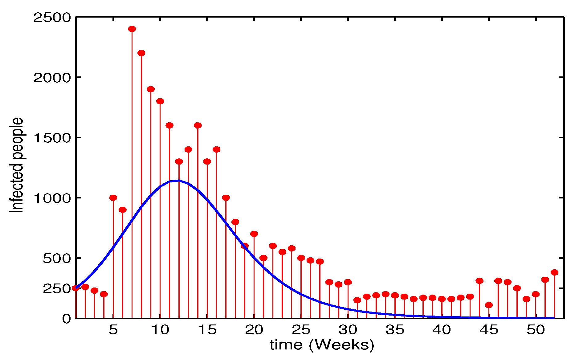
Ethiopia is one of the countries with high measles mortality burden [18]. Measles is reported weekly by the Ministry of Health. According to the Ethiopian Weekly Epidemiological Bulletin [31] report, the national surveillance data summary of measles disease in 2015 is presented in Figure 1. The real data points are represented by the red dot histogram.

5.2. Nominal Parameters

In order to simulate the proposed measles model in the context of Ethiopian data it is necessary to set all the parameter values. Some of the parameter values are obtain from national census data bases. Among these are the natural birth and death rates and the total population. The natural mortality rate for Ethiopia is

μ = 1 / (64 \times 52) {[w e e k s]}^{- 1}

[32]. Some others, such as the parameter rate of progress from exposed to infectious class (

ϵ

) and recovery rate (

γ

) are also found from measles infected patients’ clinical studies. Considering the assumption that the latent period for measles ends in

6 - 9

days and the infectious period as 5 days [33] we choose

ϵ = 7.5 / 7 {[w e e k s]}^{- 1}

and

γ = 5 / 7 {[w e e k s]}^{- 1}

5.3. Forward Problem

The system (19) can be given in vector form as:

\frac{d x (t)}{d t} = f (x (t), p), x (t_{0}) = x_{0},

(21)

where

x (t) = (S, E, I, R) \in R^{4}

represents the state variables and

x_{0} = (S (0), E (0), I (0), R (0)) \in R^{4}

is the initial condition at the initial time

t_{0}

, the vector

p = (p_{1}, p_{2}, p_{3}, p_{4}, p_{5}, p_{6}) = (Λ, β, μ, ϵ, γ, d) \in R^{6}

represents the model parameters and

f : U \subset R^{4} \times R^{6} \to R^{4}

is a nonlinear map representing the evolution law of the system defined on the open set:

\begin{matrix} U = \{(x (t), p) \in R^{4} \times R^{6} ∣ x_{i} > 0, f o r i = 1, \dots, 4 a n d p_{i} > 0, f o r i = 1, \dots, 6\} . \end{matrix}

(22)

The solution to the forward problem is obtained by numerical integration using a Runge-Kutta fourth and fifth orders (

o d e 45

) method. To simulate the forward problem we assume the initial set of parameters as

p_{0} = (500, 2.59605, 1 / (64 \times 52), 7.5 / 7, 5 / 7, 0.168)

. Initially infected humans are assumed as the number of confirmed measles cases in Ethiopia in 2015 which is

I (0) = 250

individuals. The exposed and infected groups are also equal,

E (0) = I (0)

. Moreover, initially recovered individuals are assumed to be

R (0) = 1800

. The susceptible population is also assumed to be

S (0) = 21000

. Accordingly, the initial state variables at the initial time

t_{0}

are given as

x_{0} = (21000, 250, 250, 1800)

. It is also assumed that the proportion of vaccinated in the year 2015 is

θ = 0.65

Following the above initial assumptions, Figure 1 depicts the

S E I R

model solution compared with the real data reported weekly. Apart from the numerical variation between the model solution and the real data, there exists an agreement in the pattern of the model simulation and the real data. This characteristic pattern agreement and numerical disparity proposes that the model solution may vary from the real data due to the use of improper initial parameter values or improper initial state variables in the numerical simulation. Therefore, it is important that model calibration is done to fit the model solution to the observed real data.

Figure 1. Simulation of the model solution compared to the real data using the initial parameter and state values. Observed real data points are represented by the red dot histogram and the best fitting solution curve for the system model is shown by the blue curve.

Model calibration is a numerical simulation for the search of parameter values that make the model simulation fit well with the real data. It is discussed in the following subsection.

5.4. Inverse Problem

In most cases, it is impractical the forward problem to reproduce the real data. This could be due to the error in data collection or data registration and error on model formulation caused by wrong model assumptions. Therefore, model calibration consists of seeking suitable set of parameters that, to a certain degree, makes the model solution as close as to the real data.

For the model calibration, the system contains

p = (p_{1}, p_{2}, p_{3}, p_{4}, p_{5}, p_{6})

unknown parameters to be estimated based on real data. For the purpose of comparison between the real data observations and model solutions, a discrete time set with

N = 52

weeks presented in Figure 1 is used. The N time discrete real data points are represented by

Z = (z_{1}, z_{2}, . . ., z_{N})

and the time discrete model solution

y (t_{k}) = (y_{1}, y_{2}, \dots, y_{N})

is generated for the 4 outputs

y_{1}, y_{2}, y_{3}, y_{4}

corresponding to N data points.

\begin{matrix} y (t_{k}) = {[y_{1} (t_{k}), y_{2} (t_{k}), y_{3} (t_{k}), y_{4} (t_{k})]}^{T} a n d \\ y = {[y_{1} (t_{1}), \dots, y_{1} (t_{N}), \dots, y_{4} (t_{1}), \dots, y_{4} (t_{N})]}^{T} (l e n g t h 4 \cdot N) . \end{matrix}

The model error (or the the residual error)

e_{k}

which is the difference between a column vector model solution

y

and a column vector real data points

z

is weighted in a quadratic criterion

J_{N}

\begin{matrix} e_{k} = z (t_{k}) - \hat{y} (t_{k}, \hat{p}), k = 1, \dots, N, \end{matrix}

(23)

\begin{matrix} J_{N} = | | z - {y | |}^{2} = \sum_{i = 1}^{M} e_{k}^{T} W e_{k} . \end{matrix}

(24)

In formal terms, given a real data observation vector z and a model solution vector

y

, the calibration aims at finding a vector of parameters

\hat{p}

such that

\hat{p} = a r g min_{\hat{p} \geq 0} J_{N} (\hat{p}),

(25)

for a function Equation (16). Here,

\hat{p}

is the optimal estimated parameter and

\hat{y}

is the model solution corresponding to the optimal

\hat{p}

value.

W

is a

4 \cdot N \times 4 \cdot N

positive definite symmetric weighting matrix to be solved using the weighted least squares algorithm. For the optimal estimated parameter values the functional

J_{N}

reaches a minimum value [34].

For the implementation of the calibration, we used the least squares method using the Trust-Region-Reflective method algorithm lsqnonlin from the MATLAB’s optimization Toolbox. The parameters are estimated with lower and upper bounds. Global minimum convergence is not guaranteed in this case. However, to find the best optimal parameter estimates with minimum functional value, the algorithm is started with different initial parameter and state values. The estimated parameter values are presented in Table 2 and the estimated basic reproduction number of measles for Ethiopia in the year 2015 is found out to be

R_{0} = 1.3973

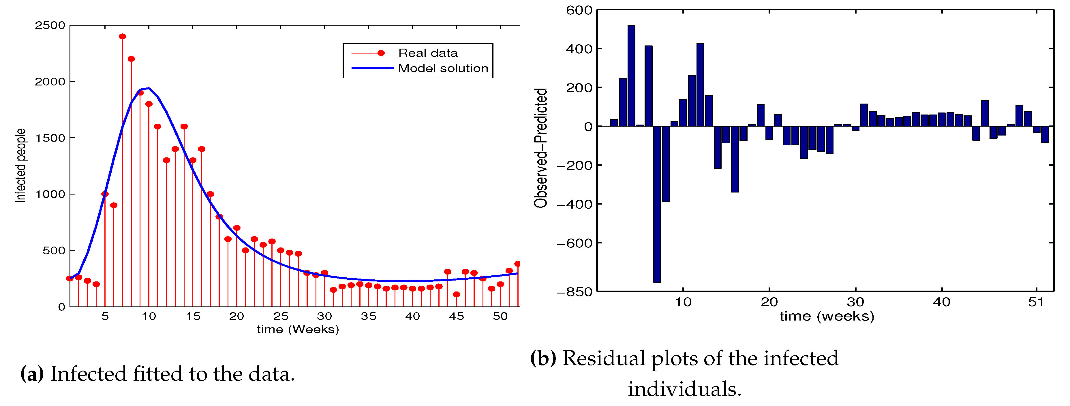
Figure 2a depicts the proposed system model fitted to real data. We found that there are only very few points that are poorly fitted with the model solution as compared. The fit of a system model to a real data is also measured by its residuals which is defined as the difference between the real data and the value predicted by the model. The residual plots seem to be random proving that the model is well calibrated (Figure 2b).

5.5. Local Sensitivity Analysis

Studying the sensitivity of the basic reproduction number as model parameters change is important in system dynamics. It is used to determine the robustness of system predictions to parameter values. A highly sensitive parameter should be carefully estimated, because a small variation in that parameter could lead to large quantitative changes. Less sensitive parameter, does not require as much effort to estimate, since a small change in that parameter will not result in a big influence in the disease dynamics.

Definition 3.

The normalized forward local sensitivity index of the basic reproduction number

R_{0 v}

that depends differentiably on a parameter

ω

is defined by

Π_{ω}^{R_{0 v}} = \frac{\partial R_{0 v}}{\partial ω} \frac{ω}{| R_{0 v} |} .

(26)

Notice that

Π_{ω}^{R_{0 v}}

has a maximum value of magnitude 1.

Π_{ω}^{R_{0 v}} = 1

implies an increase (decrease) of

ω

y %

increases (decreases)

R_{0 v}

y %

. On the other hand,

Π_{ω}^{R_{0 v}} = - 1

indicates an increase (decrease) of

ω

y %

decreases (increases)

R_{0 v}

y %

. Following Equation (26), the normalized forward local sensitivity index of

R_{0 v}

with respect to

β, μ, ϵ, γ, d, θ

is given by

\begin{matrix} Π_{β}^{R_{0 v}} & = 1, Π_{μ}^{R_{0 v}} = - \frac{μ (2 μ + ϵ + γ + d)}{(μ + ϵ) (μ + γ + d)}, Π_{ϵ}^{R_{0 v}} = \frac{μ}{μ + ϵ}, \\ Π_{γ}^{R_{0 v}} & = - \frac{γ}{μ + γ + d}, Π_{d}^{R_{0 v}} = - \frac{d}{μ + γ + d}, Π_{θ}^{R_{0 v}} = - \frac{θ}{1 - θ} . \end{matrix}

It can be easily observed from Table 3 that the local sensitivity indices of the parameters

β

and

ϵ

are positive and the remaining are negative. Positive sensitivity indices have positive result on the increase of the basic reproduction number and negative sensitivity indices have reverse effect on the basic reproduction number. The effective contact rate of measles

β

and the rate of vaccination

θ

are the most sensitive parameters and significantly impact the disease dynamics. More importantly, decreasing the effective contact rate of measles

β

and increasing the vaccination rate

θ

decrease the basic reproduction number. On the other hand, the natural death rate of humans and the rate of progress from the exposed to the infectious class are less sensitive to the basic reproduction number.

6. Numerical Simulations

6.1. The System without Vaccination

In this subsection, numerical simulations of the forward bifurcation of the system (1) and the mesh and contour plots for the basic reproduction number are discussed.

Forward Bifurcation

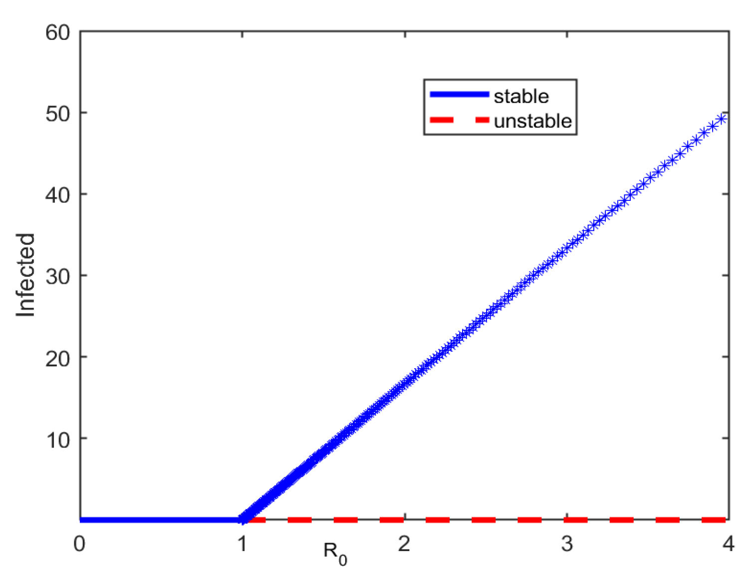
It is shown in Equation (6) that the disease dies out if

R_{0} \leq 1

and is endemic if

R_{0} > 1

for

β > d

. These results further prove that the model exhibits forward bifurcation. The global stability of the disease free and endemic equilibria for

R_{0} \leq 1

and

R_{0} > 1

, receptively is also depicted graphically in Figure 3. The dots colored in red show that the disease free equilibrium is unstable if the reproduction number is greater than unity. On the other hand, the line segment colored in blue shows that the disease free equilibrium is globally asymptotically stable if

R_{0} \leq 1

and the endemic equilibrium is globally stable if

R_{0} > 1

R_{0} = 1

is the threshold value.

Mesh and Contour Plots

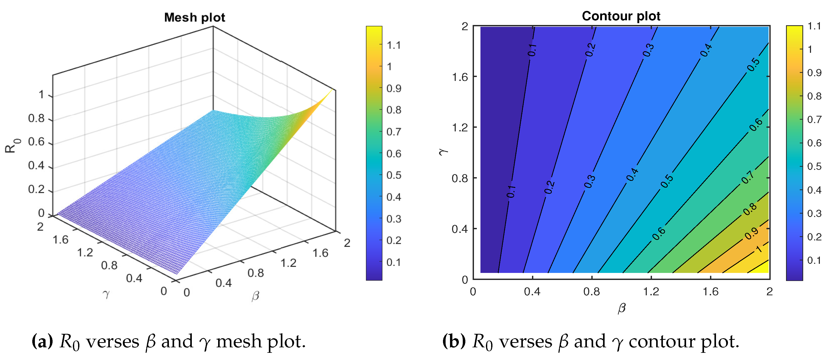
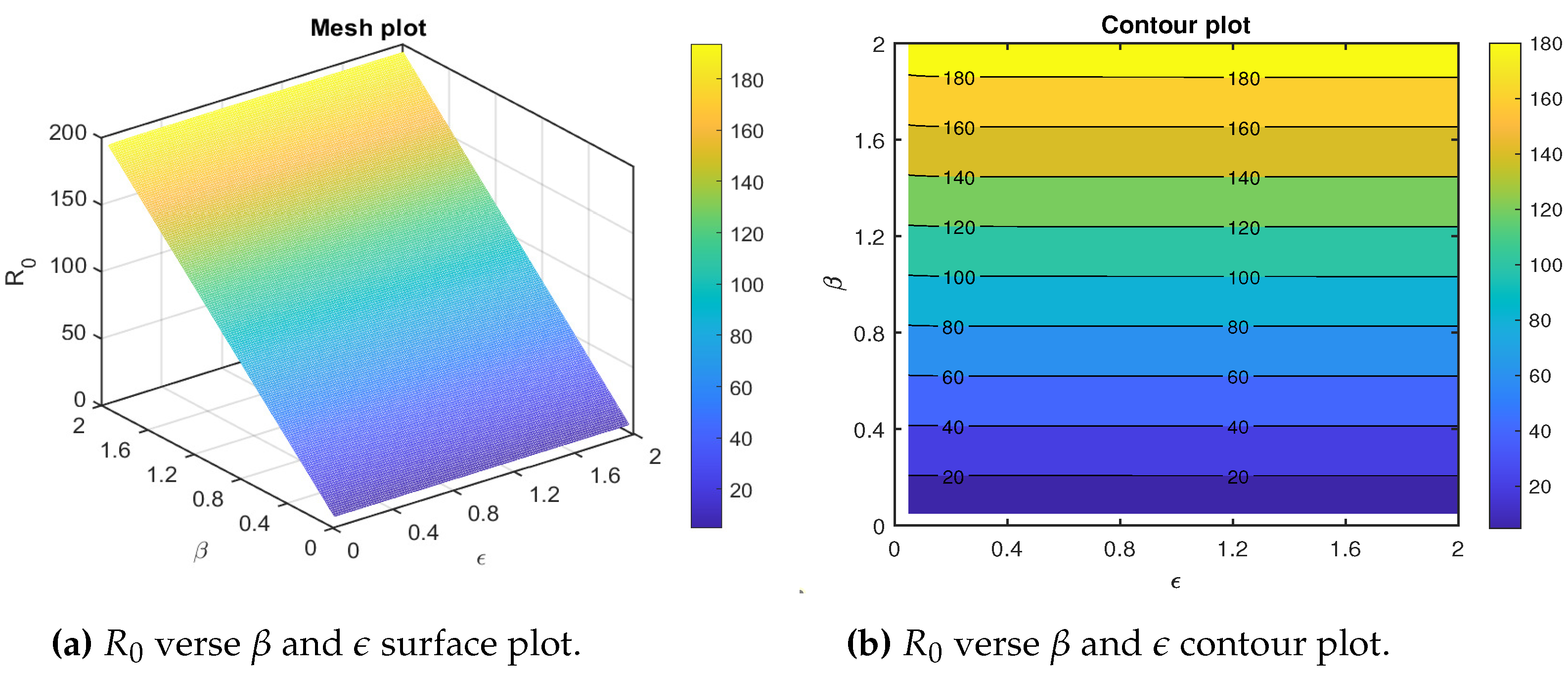
We draw the mesh and contour plots for the basic reproduction number dependence on the effective transmission rate

β

and the natural recovery rate

γ

. The mesh and contour plots show that the basic reproduction number increases significantly for higher values of

β

and lower values of

γ

(Figure 4a,b). Thus, to control

R_{0}

policymakers are recommended to work on reducing

β

and increasing

γ

. The variation of the basic reproduction number as the parameters effective transmission rate

β

and the natural recovery rate

γ

covary is depicted in Figure 4.

We also draw the mesh and contour plots for the basic reproduction number dependence on the effective transmission rate

β

and the rate of progression to the infectious class

ϵ

. The mesh and contour plots show that the basic reproduction number increases significantly for higher values of

β

, but

ϵ

has no significant value (Figure 5a,b). In this case, to control

R_{0}

policymakers are recommended to work on reducing

β

. The variation of the basic reproduction number as the parameters effective transmission rate

β

and the rate of progression to the infectious

ϵ

covary is depicted in Figure 5.

6.2. The System with Vaccination

In this subsection, numerical simulations of the proposed system (19) are done. We also validate the importance of the threshold parameter

R_{0}

to show disease elimination and endemic cases. The simulations are done using the built-in MATLAB function ode45.

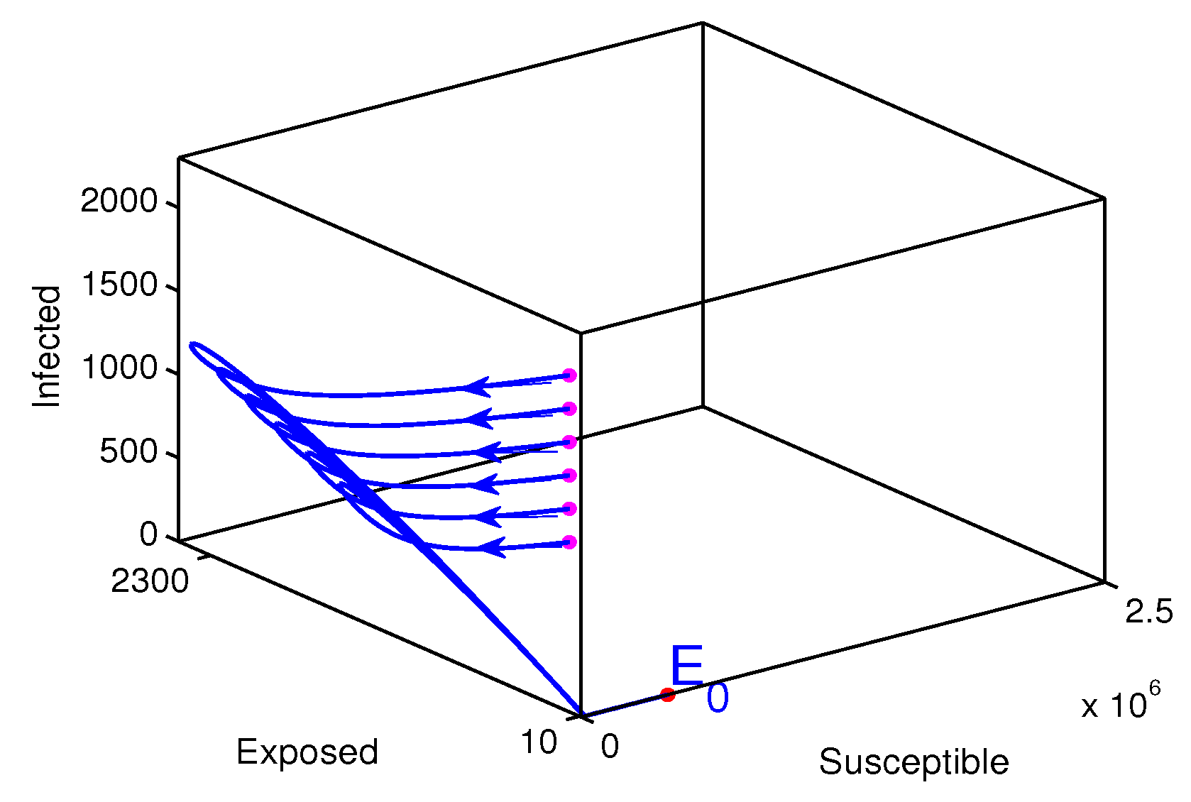
6.2.1. the Disease Extinction Case

The measles disease extinction (Figure 6). The starting points where the solution trajectories start are colored in magenta and the end point of the solution trajectories is colored in red. The direction of the solution trajectories is shown by a forward arrow. In this case the disease-free equilibrium

E_{0} =

(1690709,0,0,32123479) is globally stable. All solution values tend to move to the disease-free equilibrium what ever the initial value is. The disease free equilibrium is the plane containing the susceptible and recovered classes. From this graphical result it could be concluded that the disease dies out from the community. The calculated value of the reproduction number is

R_{0} = 0.1996

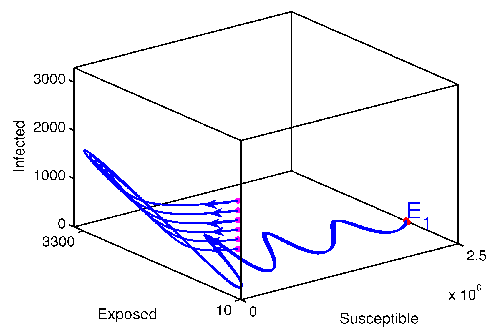
6.2.2. the Disease Endemic Case

The measles disease endemic case (Figure 7). The starting points where the solution trajectories start are colored in magenta and the end point of the solution trajectories is colored in red. The direction of the solution trajectories is shown by a forward arrow. In this case the endemic equilibrium

E^{*} =

(2250705,642,324,5601600) is globally stable. All solution values tend to move to the endemic equilibrium. From this graphical result it could be concluded that the disease is endemic. The calculated value of the reproduction number is

R_{0} = 1.3973

6.2.3. the Effects of Vaccination and Transmission Rates

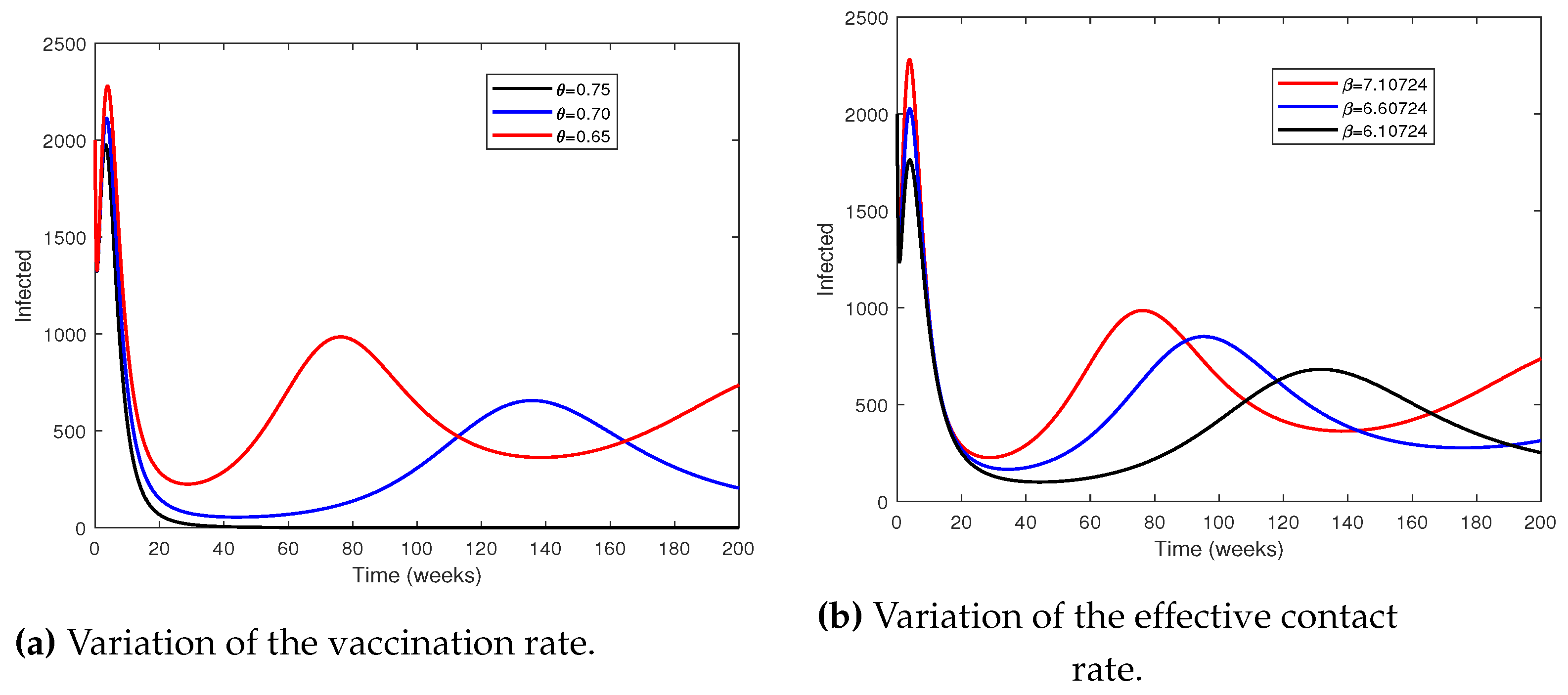
The effects of vaccination and transmission rates are discussed here. This is important to identify which one would be the most valid parameter for controlling disease spreading since both are the most sensitive parameters. Figure 8 shows the time series of the infected when the most sensitive parameters are changed. As the rate of vaccination increases from 0.65 to 0.75 it can be observed that the disease can be eradicated from the community (Figure 8a). Compared to the impact of the vaccination rate, lowering the effective contact rate from 7.10724 to 6.10724 does not have a significant impact on the eradication of the disease eradication (creffig:bettavary). The epidemiological implication of this is that vaccination of the susceptible population is the best means for controlling the disease.

It is also worth to note that the

S E I R

model assumption is not like the

S I R

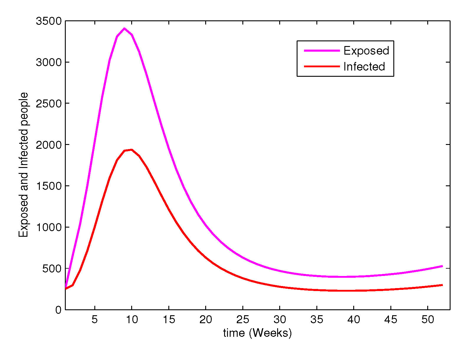
in which it cannot be concluded the disease dies out if the number of infected individuals is minimized. The time series of the exposed and infected individuals presented by Figure 9 can prove this hypothesis. It can be observed that the number of individuals in the exposed class is enormous as compared to infected ones. Even though the infected individuals seemingly to decrease which may cause ultimately the disease to die out, the disease may remain endemic due to the transfer of the exposed individuals to the infected class.

7. Discussions and Conclusions

A deterministic

S E I R

model to describe the dynamics of the measles outbreak in Ethiopia is analyzed and calibrated using weekly real data. The long-term dynamics of the system are analyzed. It is shown that the system is biologically feasible. It is also established that the

R_{0}

is a sharp threshold value and it does completely determine the global stability of the disease-free equilibrium for

R_{0} < 1

. And therefore the system exhibits forward bifurcation. Furthermore, the global stability analysis of the endemic equilibrium is analyzed for

R_{0} > 1

using a suitable Lyapunov function by assuming the disease-induced death rate

d = 0

. Based on our mathematical analysis, to eliminate the measles disease from a community, policymakers may work on reducing the basic reproduction number to less than unity. This result is different from the previous results on measles dynamics [4,20], where reducing the basic reproduction number to less than one is not enough for measles eradication. It is important to note that it is still challenging to propose an appropriate Lyapunov function to study the stability of the endemic equilibrium when

d > 0

. Therefore, further study using the Lyapunov function theory is needed to determine the global stability of the endemic equilibrium of an SEIR with standard incidence and disease-induced death rate. However, the better way to deal with so far is to use the geometric approach proposed in the works of [12].

The calibration process is done through the solution of an inverse problem using the least squares method using the Trust-Region-Reflective method algorithm lsqnonlin from MATLAB’s optimization Toolbox. Nominal initial parameter and range values are selected from the related literature studying measles disease dynamics. Estimated parameter values with 95% confidence intervals are presented. Furthermore, unlike the previous work by the authors [21] who studied the global sensitivity analysis of the basic reproduction number, local sensitivity analysis of the basic reproduction number to the estimated parameters is done to investigate the robustness of the model as parameters change. It is found that a decrease in the contact rate and an increase in the vaccination rate would cause the disease to die out.

The

S E I R

model is not like the

S I R

in that we cannot say the epidemic is in control if the number of infected individuals drops. Definitely, in the

S E I R

models, it may come about that temporarily the number of people in the infected class is small though the exposed class is still enormous. Consequently, the epidemic may appear died out but will then be out of control again when the people in the exposed class transfer to the infected class and contaminate other people. Therefore, an effective strategy essentially takes into consideration the time necessary for the exposed class to transfer to infected and will minimize to zero new infected cases throughout the period.

Like many epidemic models, the system studied has drawbacks. We calibrated the proposed model to weekly reported cases of measles to estimate the parameters of the model. Estimation of parameters is a tedious work because a large part of the infectious process is missed in most cases [35]. One of the drawbacks is that we could obtain an optimal parameter values that result in a local minimum. Therefore, to solve this problem the recommendation is to simulate the system for several sets of initial parameter values and take the optimal parameters with the smallest error as the best parameter estimate.

Even though we used a comparatively simple model of measles to demonstrate our methodology, the method that we use can be functional on a more complex models by incorporating additional information into the model. For instance, age structure would be very much suitable when considering potential vaccination strategies for measles [5,36]. Furthermore, parameter uncertainty will always exist during the estimation of the parameters and will always influence model predictions. Consequently, an age structured measles model that incorporates uncertainty analysis in the parameter estimation is essential to be investigated.

Data Availability Statement

All data relevant to this publication are within the paper.

Acknowledgments

We would like to thank the editor and the anonymous referees for their comments to improve the quality of the paper

Conflicts of Interest

The authors declare that they have no competing interests.

References

Perry, R.T.; Halsey, N.A. The Clinical Significance of Measles: A Review. The Journal of Infectious Diseases 2004, 189, S4–S16. [PubMed]
Halsey, N.A. Measles in developing countries. BMJ 2006, 333, 1234–1234. [CrossRef] [PubMed]
Anderson, R.M.; Nokes, D.J. Mathematical models of transmission and control (ch.6.14), 4 ed.; Vol. 2, New York: Oxford University Press, 2002; pp. 715–744.
Lacitignola, D. Saturated treatments and measles resurgence episodes in South Africa: A possible linkage. Mathematical Biosciences and Engineering 2013, 10, 1135–1157. [PubMed]
Anderson, R.M.; May, R.M. Age-related changes in the rate of disease transmission: Implications for the design of vaccination programmes. Journal of Hygiene 1985, 94, 365–436. [CrossRef] [PubMed]
Roberts, M.G.; Tobias, M.I. Predicting and preventing measles epidemics in New Zealand: application of a mathematical model. Epidemiology and Infection 2000, 124, 279–287. [CrossRef] [PubMed]
Gebremeskel, A.A.; Berhe, H.W.; Atsbaha, H.A. Mathematical Modelling and Analysis of COVID-19 Epidemic and Predicting its Future Situation in Ethiopia. Results in Physics 2021, 22, 103853. 103853. [CrossRef] [PubMed]
Zeb, A.; Alzahrani, E.; Erturk, V.S.; Zaman, G. Mathematical Model for Coronavirus Disease 2019 (COVID-19) Containing Isolation Class. BioMed research international 2020, 2020. [CrossRef]
Berhe, H.W.; Mo’tassem Al-arydah. Computational modeling of human papillomavirus with impulsive vaccination. Nonlinear Dynamics 2021, 103. [CrossRef]
Korobeinikov, A.; Wake, G.C. Lyapunov functions and global stability for SIR, SIRS, and SIS epidemiological models. Applied Mathematics Letters 2002, 15, 955–960. [CrossRef]
Vargas-De-León, C. Constructions of Lyapunov functions for classic SIS, SIR and SIRS epidemic models with variable population size. Revista Electrónica Foro Red Mat 2009, 26, 1–12.
Li, M.Y.; Muldowney, J.S. A Geometric Approach to Global-Stability Problems. SIAM Journal on Mathematical Analysis 1996, 27, 1070–1083. [CrossRef]
Berhe, H.W.; Makinde, O.D.; Theuri, D.M. Modelling the dynamics of direct and pathogensinduced dysentery diarrhoea epidemic with controls. Journal of Biological Dynamics 2019, 13. [CrossRef] [PubMed]
Gebremeskel, A.A.; Berhe, H.W.; Abay, A.T. A mathematical modelling and analysis of COVID-19 transmission dynamics with optimal control strategy. Computational and Mathematical Methods in Medicine 2022, 2022, 1–15. [CrossRef]
Eber, D.; Michel, T.; Americo, Cunha, J. Calibration of a SEIR-SEI epidemic model to describe the Zika virus outbreak in Brazil. Applied Mathematics and Computation 2002, 338, 955–960.
Inc, M.; Acay, B.; Berhe, H.W.; Yusuf, A.; Amir, K.; Shao-Wen, Y. Analysis of novel fractional COVID-19 model with real-life data application. Results in Physics 2021, 23, 103968. [CrossRef] [PubMed]
Berhe, H.W. Optimal Control Strategies and Cost-effectiveness Analysis Applied to Real Data of Cholera Outbreak in Ethiopia’s Oromia Region. Chaos, Solitons & Fractals 2020, 138, 109933.
Stéphane, V.; Mira, J.; Shaun, K.M.; Cindy, L.G.; Prabhat, J.; Mark, J. Controlling measles using supplemental immunization activities: A mathematical model to inform optimal policy. Vaccine 2015, xxx, xxx–xxx.
Alemneh, H.T.; Belay, A.M. Modelling, Analysis, and Simulation of Measles Disease Transmission Dynamics. Discrete Dynamics in Nature and Society 2023, 2023, 1–20. [CrossRef]
Berhe, H.W.; Makinde, O.D. Computational modelling and optimal control of measles epidemic in human population. Biosystems 2020, 190, 104102. [CrossRef]
Kuddus, M.A.; Mohiuddin, M.; Rahman4, A. Mathematical analysis of a measles transmission dynamics model in Bangladesh with double dose vaccination. Scientific reports 2021, 2021, 1–16. [CrossRef]
Pang, L.; Ruan, S.; Liu, S.; Zhao, Z.; Zhang, X. Transmission dynamics and optimal control of measles epidemics. Applied Mathematics and Computation 2015, 256, 131–147. [CrossRef]
Peter, O.J., P.H.I.M.e.a. Analysis and dynamics of measles with control strategies: A mathematical modeling approach. Int. J. Dynam. Control 2023, pp. 1–16.
Bonyah, E.; Khan, M.; Okosun, K.; Gomez-Aguilar, J. Modelling the effects of heavy alcohol consumption on the transmission dynamics of gonorrhea with optimal control. Mathematical Biosciences 2019, 309, 1–11. [CrossRef]
van den Driessche, P.; Watmough, J. Reproduction numbers and subthreshold endemic equilibria for compartmental models of disease transmission. Mathematical Biosciences 2002, 180, 29–48. [CrossRef]
Arino, J.; McCluskey, C.C.; van den Driessche, P. Global Results for an Epidemic Model with Vaccination that Exhibits Backward Bifurcation. SIAM Journal on Applied Mathematics 2003, 64, 260–276. [CrossRef]
LaSalle, J. Stability theory for ordinary differential equations. Journal of Differential Equations 1968, 4, 57–65. [CrossRef]
Kot, M. Elements of Mathematical Ecology. Cambridge University Press 2001.
La Salle, J.P. The stability of dynamical systems; SIAM, 1976.
Castillo Chavez, C.; Song, B. Dynamical Models of Tuberculosis and Their Applications. Mathematical Biosciences and Engineering 2004, 1, 361–404. [CrossRef]
Abyot Bekele, M. Ethiopian Public Health Institute Center for Public Health Emergency Management. Ethiopian Weekly Epidemiological Bulletin 2016, 2, 6–7.
Life expectancy at birth, total Ethiopian data in the years 1960–2017, 2020. https://data.worldbank.org/indicator/SP.DYN.LE00.IN.
Balker, B. Chaos and complexity in measles models: A comparative numerical study. IMA Journal ofMathematics Applied in Medicine & Biology 1993, 10, 83–95.
Riel, V.; Real. Parameter estimation in non-equidistantly sampled nonlinear state space models; a Matlab implementation 2006. pp. 1–16.
Berhe, H.W.; Makinde, O.D.; Theuri, D.M. Co-dynamics of measles and dysentery diarrhea diseases with optimal control and cost-effectiveness analysis. Applied Mathematics and Computation 2019, 347, 903–921. [CrossRef]
Anderson, R.M.; May, R.M. Vaccination against rubella and measles: Quantitative investigations of different policies. Journal of Hygiene 1983, 90, 259–325. [CrossRef] [PubMed]

Figure 2. The

S E I R

system fitted with the weekly reported real data. Observed real data points are represented by the red dot histogram and the best fitting solution curve for the system model is shown by the blue curve.

Figure 2. The

S E I R

Figure 3. The forward bifurcation graph for infected versus

R_{0}

using the parameters

Λ = 100, β = 6, μ = 0.00045662, ϵ = 0.01, d = 0.0015

and

γ

varies between 0.01 and 20, i.e,

γ = 0.01 : 0.005 : 20

Figure 3. The forward bifurcation graph for infected versus

R_{0}

using the parameters

Λ = 100, β = 6, μ = 0.00045662, ϵ = 0.01, d = 0.0015

and

γ

varies between 0.01 and 20, i.e,

γ = 0.01 : 0.005 : 20

Figure 4. Combined effects of the transmission rate

β

and the recovery rate

γ

on the basic reproduction number for the measles model. The parameters both vary in the interval

β = 0.05 : . 02 : 2

and

γ = 0.05 : . 02 : 2

. The remaining parameters are given in Table 2.

Figure 4. Combined effects of the transmission rate

β

and the recovery rate

γ

on the basic reproduction number for the measles model. The parameters both vary in the interval

β = 0.05 : . 02 : 2

and

γ = 0.05 : . 02 : 2

. The remaining parameters are given in Table 2.

Figure 5. Combined effects of the effective transmission rate

β

and the rate of progression to the infectious class

ϵ

on the basic reproduction number for the measles model. The parameters

β

and

ϵ

vary in the interval

β = 0.05 : . 01 : 2

and

ϵ = 0.05 : . 01 : 2

. The remaining parameters are given in Table 2.

Figure 5. Combined effects of the effective transmission rate

β

and the rate of progression to the infectious class

ϵ

on the basic reproduction number for the measles model. The parameters

β

and

ϵ

vary in the interval

β = 0.05 : . 01 : 2

and

ϵ = 0.05 : . 01 : 2

. The remaining parameters are given in Table 2.

Figure 6. Solution trajectories for the disease free equilibrium. In this case the assumed initial state value is

(S (0), E (0), R (0)) = (21000, 250, 18000)

while varying the initial infected individuals between 1000 and 2000 with step size 200, the rate of vaccination is also assumed to be

θ = 0.95

, and the estimated parameters values are

Λ = 9.289613942105396 \times 10^{3}, β = 0.007107 \times 10^{3}, ϵ = 0.001024 \times 10^{3}, μ = 0.0000002747 \times 10^{3}, γ = 1, d = 0.0007795 \times 10^{3}

Figure 6. Solution trajectories for the disease free equilibrium. In this case the assumed initial state value is

(S (0), E (0), R (0)) = (21000, 250, 18000)

while varying the initial infected individuals between 1000 and 2000 with step size 200, the rate of vaccination is also assumed to be

θ = 0.95

, and the estimated parameters values are

Λ = 9.289613942105396 \times 10^{3}, β = 0.007107 \times 10^{3}, ϵ = 0.001024 \times 10^{3}, μ = 0.0000002747 \times 10^{3}, γ = 1, d = 0.0007795 \times 10^{3}

Figure 7. Solution trajectories for the endemic equilibrium. In this case the assumed initial state value is

(S (0), E (0), R (0)) = (21000, 250, 18000)

while varying the initial infected individuals between 1000 and 2000 with step size 200, the rate of vaccination is assumed to be

θ = 0.65

, and the estimated parameters values are

Λ = 9.289613942105396 \times 10^{3}, β = 0.007107 \times 10^{3}, ϵ = 0.001024 \times 10^{3}, μ = 0.0000002747 \times 10^{3}, γ = 1, d = 0.0007795 \times 10^{3}

Figure 7. Solution trajectories for the endemic equilibrium. In this case the assumed initial state value is

(S (0), E (0), R (0)) = (21000, 250, 18000)

while varying the initial infected individuals between 1000 and 2000 with step size 200, the rate of vaccination is assumed to be

θ = 0.65

, and the estimated parameters values are

Λ = 9.289613942105396 \times 10^{3}, β = 0.007107 \times 10^{3}, ϵ = 0.001024 \times 10^{3}, μ = 0.0000002747 \times 10^{3}, γ = 1, d = 0.0007795 \times 10^{3}

Figure 8. Time series of the infected population by varying the vaccination and effective contact rates.

Figure 9. The time series of the exposed and infected people. In this case the assumed initial state value is

(S (0), E (0), I (0), R (0)) = (21000, 250, 250, 18000)

. The rate of vaccination is assumed to be

θ = 0.65

and the estimated parameters values are

Λ = 9.289613942105396 \times 10^{3}, β = 0.007107 \times 10^{3}, ϵ = 0.001024 \times 10^{3}, μ = 0.0000002747 \times 10^{3}, γ = 1, d = 0.0007795 \times 10^{3}

Figure 9. The time series of the exposed and infected people. In this case the assumed initial state value is

(S (0), E (0), I (0), R (0)) = (21000, 250, 250, 18000)

. The rate of vaccination is assumed to be

θ = 0.65

and the estimated parameters values are

Λ = 9.289613942105396 \times 10^{3}, β = 0.007107 \times 10^{3}, ϵ = 0.001024 \times 10^{3}, μ = 0.0000002747 \times 10^{3}, γ = 1, d = 0.0007795 \times 10^{3}

Table 1. Description of parameters of system. (1)

Parameters	Interpretation	Units
$Λ$	Recruitment rate of susceptible population by immigration or birth	[Humans] ${[week]}^{- 1}$
$β$	Effective contact rate of measles	${[week]}^{- 1}$
$μ$	Natural death rate of humans	${[week]}^{- 1}$
$ϵ$	Rate of progress from exposed to infectious class	${[week]}^{- 1}$
d	Disease induced death rate of measles	${[week]}^{- 1}$
$γ$	Natural recovery rate from measles	${[week]}^{- 1}$

Table 2. Estimated parameter values for the proposed model

Parameter	Lower bound	Upper bound	Reference	Estimated value(CI)
$Λ$	0	10000	Assumed	0.9289613942(-0.1423810 2.0003038) $\times 10^{4}$
$β$	0	100	Assumed	0.0007107243(-0.0002338 0.0016552) $\times 10^{4}$
$μ$	$1 / (70 \times 52)$	$1 / (60 \times 52)$	[32]	0.0000000275(-0.0000086 0.0000087) $\times 10^{4}$
$ϵ$	$6 / 7$	$9 / 7$	[4,33]	0.0001024338(-0.0000335 0.0002384) $\times 10^{4}$
$γ$	$6 / 7$	1	[4,33]	0.0001000000(-0.0009732 0.0011732) $\times 10^{4}$
d	0	1	Assumed	0.0000779494(-0.0009738 0.0011297 ) $\times 10^{4}$

Table 3. Numerical value of the local sensitivity indices

Parameters	Local sensitivity indices
$β$	$Π_{β}^{R_{0 v}} = 1$
$μ$	$Π_{μ}^{R_{0 v}} = - 4.224877 \times 10^{- 4}$
$ϵ$	$Π_{ϵ}^{R_{0 v}} = 2.681276111938502 \times 10^{- 4}$
$γ$	$Π_{γ}^{R_{0 v}} = - 0.561870756205265$
d	$Π_{d}^{R_{0 v}} = - 0.437974883669988$
$θ$	$Π_{θ}^{R_{0 v}} = - 1.857143$

Disclaimer/Publisher’s Note: The statements, opinions and data contained in all publications are solely those of the individual author(s) and contributor(s) and not of MDPI and/or the editor(s). MDPI and/or the editor(s) disclaim responsibility for any injury to people or property resulting from any ideas, methods, instructions or products referred to in the content.

© 2023 by the authors. Licensee MDPI, Basel, Switzerland. This article is an open access article distributed under the terms and conditions of the Creative Commons Attribution (CC BY) license (http://creativecommons.org/licenses/by/4.0/).

Copyright: This open access article is published under a Creative Commons CC BY 4.0 license, which permit the free download, distribution, and reuse, provided that the author and preprint are cited in any reuse.

MDPI Initiatives

Important Links

Choose an area of interest and we will send you notifications of new preprints at your preferred frequency.

Disclaimer

Modelling and Stability Analysis of the Dynamics of Measles with Application to Ethiopian Data

Abstract

1. Introduction

2. Mathematical Model Formulation

3. Model Analysis

3.1. Nonnegativity of Solutions and the Feasible Region

3.2. Positively Invariant

3.3. Equilibria and the Basic Reproduction Number

3.4. Local Stability Analysis of Disease-Free Equilibrium

3.5. Global Stability of Disease-Free Equilibrium

3.6. Local Stability of Endemic Equilibrium

3.6.1. Global Stability of Endemic Equilibrium

4. Bifurcation Analysis

5. Model Calibration with Vaccination

5.1. Data

5.2. Nominal Parameters

5.3. Forward Problem

5.4. Inverse Problem

5.5. Local Sensitivity Analysis

6. Numerical Simulations

6.1. The System without Vaccination

Forward Bifurcation

Mesh and Contour Plots

6.2. The System with Vaccination

6.2.1. the Disease Extinction Case

6.2.2. the Disease Endemic Case

6.2.3. the Effects of Vaccination and Transmission Rates

7. Discussions and Conclusions

Data Availability Statement

Acknowledgments

Conflicts of Interest

References

MDPI Initiatives

Important Links

Subscribe