Preprint
Article

Machine-Learning Based Modelling of Air Temperature in the Complex Environment of Yerevan City, Armenia.

Altmetrics

Downloads

105

Views

45

Comments

0

A peer-reviewed article of this preprint also exists.

Submitted:

01 April 2023

Posted:

07 April 2023

You are already at the latest version

Alerts
Abstract
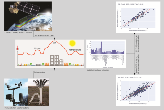
Machine Learning (ML) was used to assess and predict urban air temperature (Tair) considering the complexity of the terrain features in Yerevan (Armenia). The estimation was performed based on the PLSR model with a high number (30) of input variables. The relevant parameters include a newly purposed modification of spectral index IBI-SAVI, which turned out to be strongly impacting on Tair prediction together with land surface temperature (LST). Cross-validation analysis on temperature predictions across a station-centered 1000m circular area revealed quite a high correlation (R2Val = 0.77, RMSEVal = 1.58) between predicted and measured Tair from the test set. It was concluded the remote sensing is an effective tool to estimate Tair distribution where a dense network of weather stations is not available. However, further developments will include incorporation of additional weather parameters from the weather stations such as precipitation and wind speed, and the use of non-parametric ML techniques.
Keywords: 
Subject: Environmental and Earth Sciences  -   Remote Sensing

1. Introduction

Air temperature (Tair) is a climate variable describing the energy and thermal balance in a very special zone of the Earth-atmosphere system, namely the surface of the Earth which is at the same time the very bottom layer of the atmosphere [1]. It is a useful factor in tracking the climate change associated with human activities, especially in urban areas, which represent the “peaks” of anthropogenic activities and where the climate change impact is expressed and sensed the most. Tair is usually recorded by weather stations, which measure Tair between 1.5 - 2 m above ground and are distributed sparsely, thus failing to provide synoptic spatial coverage [2,3]. Moreover, urban areas are more heterogeneous than rural areas, hence the effective coverage of weather stations providing long-term observational data tends to be narrow [4,5], leaving large swathes of urban are-as unobserved. This is a reason to use remote sensing data for Tair prediction; remote sensing offers a possibility to track its seasonal behavior and especially its spatial distribution. Tair cannot be observed directly from space but thermal infrared sensors enable derivation of land surface temperature (LST), which is a limiting condition for the energy balance and is widely used to assess the spatial distribution of Tair [6,7].
The methodologies and approaches to assess and predict Tair via remote sensing are different. They are mainly based on a hybrid methodology, which combines GIS and re-mote sensing data. For example, in 2008 Cristobel J et al. applied this methodology combining geographical variables (e.g. altitude, latitude, continentality and solar radiation) and remote sensing predictors related with Tair such as albedo and LST and vegetation index NDVI obtained from Landsat sensors NOAA and TERRA (MODIS) and used multiple regression analysis and spatial interpolation techniques for data processing. The au-thors support that this combined approach underpins the best Tair models and NDVI and LST are the most powerful RS predictors in Tair modeling [8].
It is worth to recall that LST is a basic physical parameter to describe ecological, hydrological and atmospheric processes and has a strong relationship with near surface Tair. However, these two parameters have different responses to atmospheric conditions and their link becomes even more complex in mountainous complex terrain, and/or where weather stations are scarce. In 2020 Mutiibwa D et al analyzed the benefits and some limitations of using LST as a variable for predicting Tair in two case study regions of Nevada well known for complex mountainous topography. Though with some limitations and complexities, the relationship between LST and Tair was found to be consistent [9].
In 2020 Nikoloudakis N et al. applied the hybrid methodology to predict Tair in urban areas without LST. They developed and used predictive models, which are based on urban morphological peculiarities such as land cover and terrain, and in situ Tair measurements from urban weather stations [10].
The modeling of urban Tair is much more complicated because of the heterogeneity, where the scarcity of weather stations hinders accurate spatial representation of Tair [11]. It is further complicated in mountainous urban areas [12]. The use of Machine learning (ML) approaches increases the accuracy of the estimations of Tair [13]. A wide variety of statistical and ML models have been used so far. Among them the most popular ones still remain multiple regression, ANN models [1,11,12,14,15,16], with differences in results mainly due to the selection of input variables.
A most important component of regression models is the number of variables, which can range from one to a few tens. For example, up to 7 variables (skin temperature (LST), elevation, the Normalized Difference Water Index (NDWI), Sky View Factor (SVF), incident solar radiation, distance from the ocean, and atmospheric water vapor) were used by Hung Chak [17], 24 variables by Modeste Meliho (ACDC (Aqua day clear-sky coverage), ACNC (Aqua night clear-sky coverage), ADVA (Aqua day view angle), ADVT (Aqua day view time), AE31 (Aqua Band 31 Emissivity),AE32 Aqua Band 32 Emissivity, ALSTD (Aqua day land surface temperature), ALSTN (Aqua night land surface temperature), ANVA (Aqua night view angle), ANVT (Aqua night view time),TCDC (Terra day clear-sky coverage),TCNC (Terra night clear-sky coverage), TDVA (Terra day view angle), TDVT (Terra day view time),TE31 (Terra Band 31 Emissivity), TE32 (Terra Band 32 Emissivity),TLSTD (Terra day land surface temperature), TLSTN (Terra night land surface temperature), TNVA (Terra night view angle), TNVT(Terra night view time), Elevation (DEM), Hillshade (HSD), Sky-view, Slope) [1], 10 variables by Hanna Meyer (LST, DEM, Slope, aspect, sky-view, month, season, time, sensor, ice) [18], 11 variables by Yongming Xu (monthly daytime Ts, monthly nighttime Ts, monthly percent of cloudy days, monthly percent of cloudy nights, monthly NDVI, monthly NDSI, monthly albedo, monthly solar radiation, annual landcover, elevation, and TI) [19], 6 variables by Phan Thanh Noi (AQUA daytime, AQUA nighttime, TERRA daytime, and TERRA nighttime) and two additional auxiliary datasets (elevation and Julian day)), 5 variables by Long Li (Daytime LST, Night-time LST, NDVI, Night-time light, DEM) [20], 9 variables by Yongming Xu (land surface temperature (LST), normalized difference vegetation index (NDVI), modified normalized difference water index (MNDWI), latitude, longitude, distance to ocean, altitude, albedo, and solar radiation) [19], up to 10 variables by Munkhdulam Otgonbayar (daytime and nighttime LST data (LSTd and LSTn), quality information (QCd and QCn), observation information (DvA, NvA, DvT, and NvT), emissivity data (Em31 and Em32), clear sky coverage (CsD and CsN), Elevation, Slope, Aspect, Latitude, Longitude) [21], 7 variables by Chunling Wang (Digital elevation model (DEM), LST, Downward Shortwave Radiation (DSR), Normalized Difference Vegetation Index (NDVI), and Land Cover (LC), latitude (LAT) and declination of the sun) [22].
In this study, a PLSR model was used to assess and predict urban Tair considering more than 30 variables. To the best of our knowledge, statistical regression models starting from 30 variables have not been presented elsewhere in existing literature.
One more difference with the urban study cases described above lies in the complexity of the mountain features with respect to the size of the considered area, and the sparse configuration of weather stations. This study focuses on the city of Yerevan, Armenia, which stands out for unique geographical parameters, in particular for the high variation range of absolute elevation, exceeding 500m (>1600ft) on a small area covering about 220 sq km. The area has a dry climate, and only 3 weather stations are operating, which limits the information on spatial variation of Tair. In other case studies from literature, like Athens and Heraklion (Greece), Los Angeles (USA), Seoul (South Korea), Vancouver (Canada), Erbil (Iraq), where Tair predictions were performed using remote sensing data [10,12,16,23] such a combination is never found.
Hence, the objectives of the current study are:
  • Considering the complexity of the terrain configuration in Yerevan, to assess for the first time the feasibility of estimating urban Tair based on remote sensing data alone
  • Estimate the Urban Tair of the city of Yerevan using the PLSR model with a high (30) number of input variables.
To the best of our knowledge, so far, no investigations have been performed that could answer these questions.

2. Materials and Methods

2.1. Test site, description and terrain/climate features

Yerevan is the capital of Armenia, covering an area of approximately 220 km2 with 1.1 million inhabitants, which represents 36% of the total population and 56% of urban population. The density of population in Yerevan exceeds 4900 inhabitants/km2 [24].
Yerevan lies on a plain on the edge of the Ararat Valley at altitudes of 850–1.400 m (Figure 1). It has a dry continental climate. The average annual Tair is between 9.1 ⁰C and 12.1 ⁰C, with a seasonal fluctuation of 27 ⁰C between average summer and winter temperatures. Winters are cold with a lot of snowfall and average temperatures in January ranging between - 5 ⁰C and - 2.5 ⁰C, with absolute minimum Tair between - 21⁰C and - 31⁰C. Springs are brief, characterized by volatile weather. Summers are long, hot and dry, with average Tair between 22.1 and 25.4 ⁰C. The absolute maximums of Tair registered in July are between 40⁰C and 43⁰C [25,26]. The study area is located in the dry subtropical climate zone. Thus, climate change is especially expressed in increasing amplitude of urban Tair swings, as discussed later.
During summer, winds blowing from the mountains (north-east) to the valley (south-west) sometimes reach a speed of 15–20 m/s. The duration of the heating season is between 137 and 161 days. Annual rainfall is 286–440 mm peaking in November while the highest share of rainy days is in May. Yerevan also enjoys a lot of sunshine. The annual average of sunshine is 2578 h. Hours of sunshine per day will vary from an average of 7 in winter to 13 in summer [26].
Figure 1 shows the geographical location of Yerevan on the territory of Armenia reflecting the mountainous character of the surface. The figure also shows an unequal distribution of weather stations, which are located in the north and west of the city on different altitudes (see Table 1). As mentioned above, this pattern limits the possibility to observe spatial variations of Tair.
Since the late 80s, land cover in Yerevan has been changing rapidly, which results in potential sharpening of the natural conditions of the city on the recent climate changes. The last national communication on climate change shows that in 1981–2013 the summer heat wave in Yerevan has increased about 40 days on average [27,28]. Some studies were conducted to investigate the reasons. For instance, Tepanosyan et al. investigated the influence of spatial-temporal changes of land cover on the territory of Yerevan city on the surface urban heat, using time series of remote sensing data (Landsat TM/ETM+/OLI-TIRS images) [26]. However, no studies have been conducted so far on developing approaches to enhance visualization and to monitor spatial-temporal variation of Tair using remote sensing data and technologies for this area.

2.2. Preparation of input data

2.2.1. Satellite data

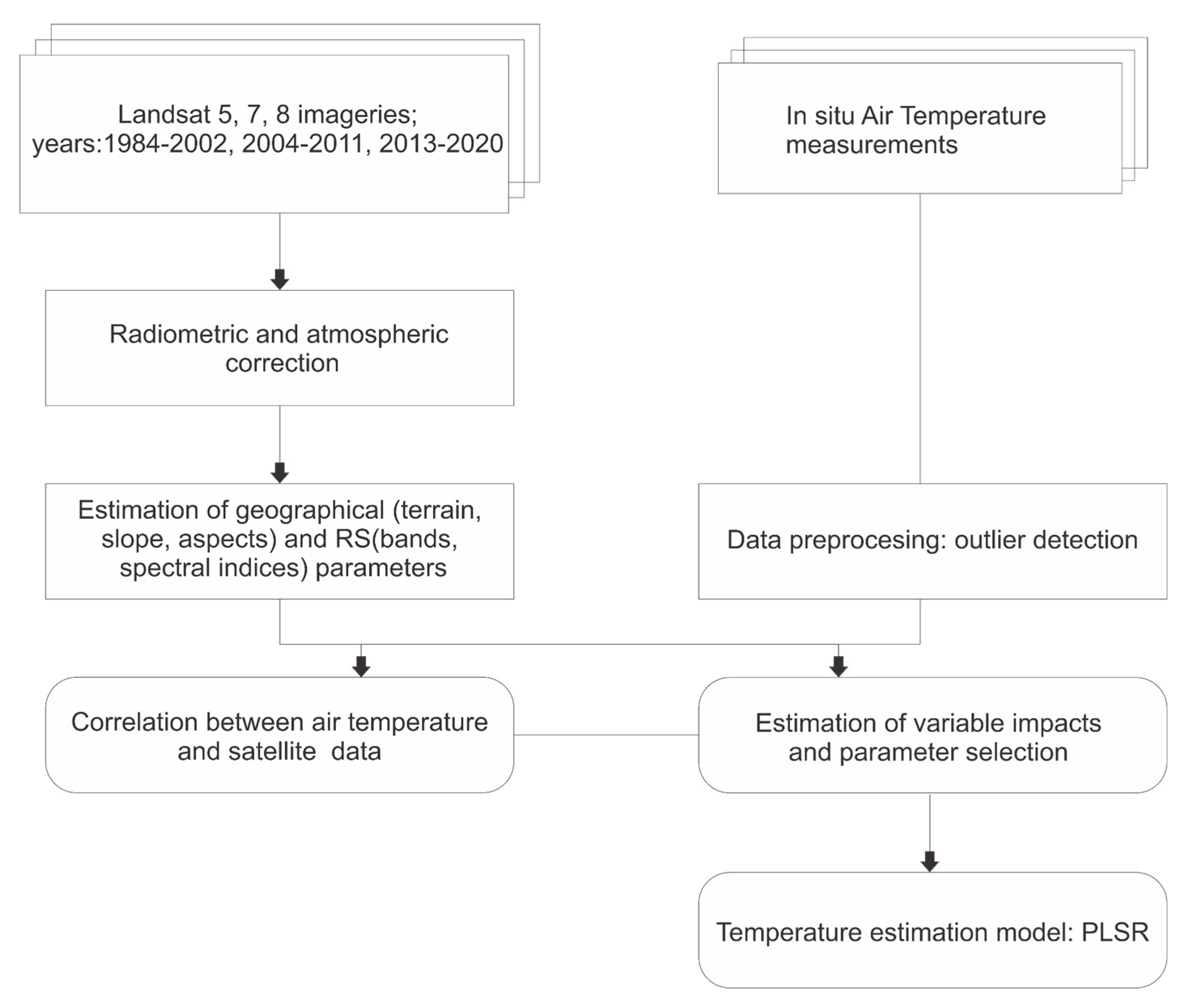
Figure 2 shows the steps of the study. The input data consists of open-source remote sensing (RS) surface reflectance products from LANDSAT 4-5TM; 7ETM; 8 OLI/TIRS covering the season from June to August for years between 1984-2020, obtained and directly processed in Google Earth Engine (GEE). Two gaps can be observed in the time sequence in 2003 and 2012; the corresponding data was discarded due to low quality. Cloud mask and cloud filtering were implemented using the CFMASK algorithm, as well as a per-pixel saturation mask [29]. Spectral indices also were calculated to complement the list of input data, which consisted of Normalized Difference Vegetation Index-NDVI, Normalized Difference Water Index - NDWI, and Index based Buildup Index-Soil adjusted vegetation index (IBI-SAVI) (1).
(((NDBI + 1) - ((SAVI + 1) + (MNDWI + 1)) / 2)) / (((NDBI + 1) + ((SAVI + 1) + (MNDWI + 1)) / 2))
The IBI-SAVI is a combined indicator, which we propose for use in this context. It is calculated from Normalized Difference Build-up Index -NDBI, SAVI, Modified Normalized Difference Water Index-MNDWI. The formula was modified partly following suggestions by Xu [30], and introducing further changes in rescaling SAVI to match the other rescaled indexes.
The LST for each year as an input data was calculated using Landsat LST Web Application. This online web application provides fast and easy access to the global scale LST from the Landsat archives based on the single channel (SC) algorithm [26,31,32,33]. Input data contains also geographical data such as elevation and its derivatives (aspects, slopes). Solar radiation was also modeled from DEM and sun location using area solar radiation toolset of ArcMap. The elevation ruggedness is calculated as Terrain Ruggedness Index, which is used to characterize the elevation difference of the DEM's adjacent cells [34]. Several single bands (RGB, NIR, SWIR1/2) of RS data complement the list of the input data.
Weather data (Tair, cloud cover, dew point, wind direction, wind speed, solar radiation) have been acquired from Armenia State Hydromet Service for three weather stations (Figure 1). We decided not to include precipitation as it is reputed to have a delayed effect on temperature, and it would not introduce additional relevant information. The dates of measurements were selected to match the dates of RS data acquisition as closely as possible. However, only two stations cover the whole considered time period (1984-2020); the third station (Yerevan-Aerology) covers only years between 2011-2020.
As Tepanosyan et al. stated, several approaches are possible when studying the relationship between RS data and climatic factors [26]. According to the first approach, maps of the several climatic parameters should be produced using interpolation methods, which requires data from a sufficient number of weather stations. In our case, the terrain shape and very few weather stations make this approach not viable [35,36,37,38]. The second approach implies studying relationships between climatic data from weather stations and average Spectral index values obtained from pixels surrounding the respective stations [39,40]. In this case study the second approach was used and mean NDVI, NDWI, IBI-SAVI values across a station-centered circular area were extracted; using multitemporal data, a time series was formed for each station. Many studies accepted 3 × 3 pixels window size as the optimal one for deriving average values of the spectral indices such as NDVI [39,40]; in this study the averaged values were instead calculated over differently sized circular windows around the weather stations. The rationale was to investigate the spatial dependence of the parameter impact; the selected sizes were 30m, 100m, 200m, 300m, 400m, 500m, 600m, 700m, 800m, 900m, 1000m. Further increase of the radius results in an overlap of the areas between two weather stations.

2.2.2. Weather data

As explained in section 2, we considered weather data from 3 weather stations located in or around Yerevan. In this paper we limited ourselves to considering Tair. Investigations about other possible weather variables will be the subject of the future work.
Initially we considered all measurements, whereas at a successive stage outlier were removed before reprocessing.
In order to detect potential outliers among data, the boxplot technique was used: parameter values that were outside the (Quartile 1 – 1.5 * Interquartile range) - (Quartile 3 + 1.5 * Interquartile) range were considered as outlier candidates. However, only acquisitions labeled as outlier candidates on all parameters were finally considered outliers and removed. All other candidates i.e. outside the range but not on all variables were still retained. This was done to ensure that only data items that could be considered outliers with a high degree of confidence were removed.

3. Statistical analysis and modeling

To study the relationships between Tair and satellite data, a Pearson correlation analysis including significance estimation was first carried out to identify the best candidates to contribute to Tair estimation. For this purpose, the calculated mean and standard deviation (SD) values of the components/variables were input. At this level, however, no actual parameter selection was done, leaving it to an automated process to be implemented at a later stage.
All statistical analyses were done using the Python programming language using Jupyter. Linear regression (LR) was implemented by Scikit learn algorithm “LinearRegression” [41]. Tair prediction was treated as a supervised regression problem. Therefore, the Partial Least-Squares Regression (PLSR) was selected in this research as the statistical approach for evaluation. For all models, the input dataset was randomly split into training (75%) and testing (25%) sets.
PLSR regression was run considering various possible combinations of the input parameters, starting from a single variable and progressively increasing the number of variables. The Variable Importance in Projection (VIP) scores were used to prioritize selections of input variables. VIP scores estimate the importance of each variable in the projection used in a PLSR model and is often used for variable selection. A variable with a VIP score close to or greater than 1 (one) can be considered important in a given model [21,42].
Each combination was tested for Mean Square Errors in predicting the training set. It was found that the optimal MSE values were obtained for 10 variables.
Further expansion of the input set did not lead to any improvement in MSE, which actually worsened. The input set to the prediction process was then set to the list above, and predictions were compared with the test set.

4. Results and discussions

Pearson values are reported in Table 2. The reported figures suggest that LST-mean has the most significant influence (r=0.79; p<0.001) on Tair. All other components such as IBI-SAVI-mean (r=0.35; p<0.001), SWIR1-mean (r≈0.3; p<0.001), SWIR2I-mean (r≈0.3; p<0.001), Red-mean (r≈0.3; p<0.001) show significant positive correlation. Green-mean, Blue-means and Aspect_SD correspondingly (r≈0.2; p<0.001), (r≈0.14; p<0.01) and (r≈0.11; p<0.01) also show significant positive correlation with Tair. Some other components such as NDWI_mean (r= -0.35; p<0.001), NDVI_mean (r= -0.25; p<0.001), NDWI_SD (r= -0.24; p<0.001) NDVI_SD (r= -0.26; p<0.001), IBI SAVI_SD and SWIR2_SD (r= -0.13; p<0.001) show significant negative correlation with Tair. In fact, two components contribute the most information to the temperature prediction and one of them is the modified IBI-SAVI index. This will be compared with results of automated selection as explained in the following.
As mentioned above the spatial dependence of the parameter impact was investigated for the selected sized areas 30m, 100m, 200m, 300m, 400m, 500m, 600m, 700m, 800m, 900m, 1000m through PLSR estimation. The table below shows the estimation results for the all-sized areas. Prior to the PLSR run the estimation of variable impacts and the selection of the parameters (VIP) were conducted.
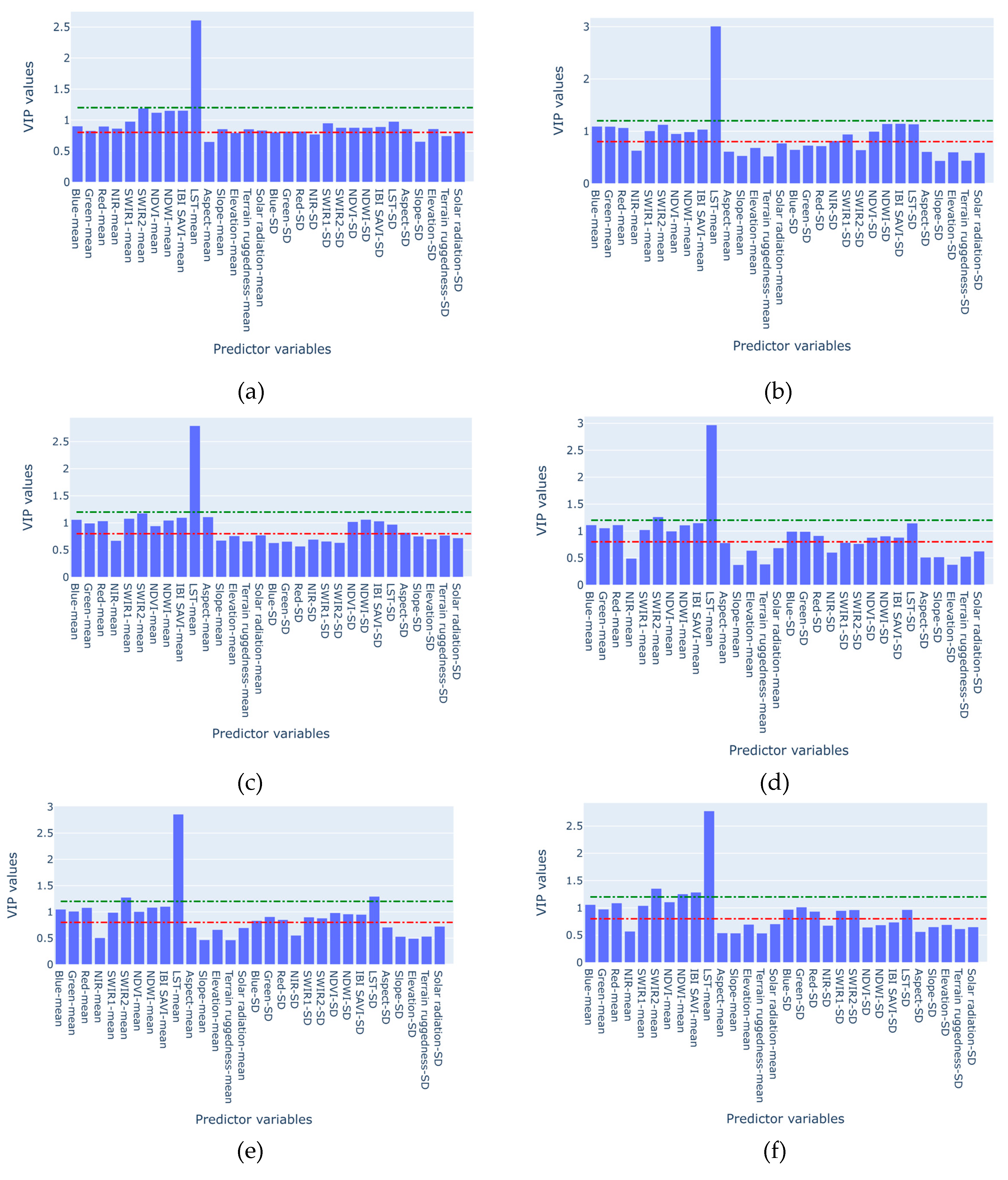
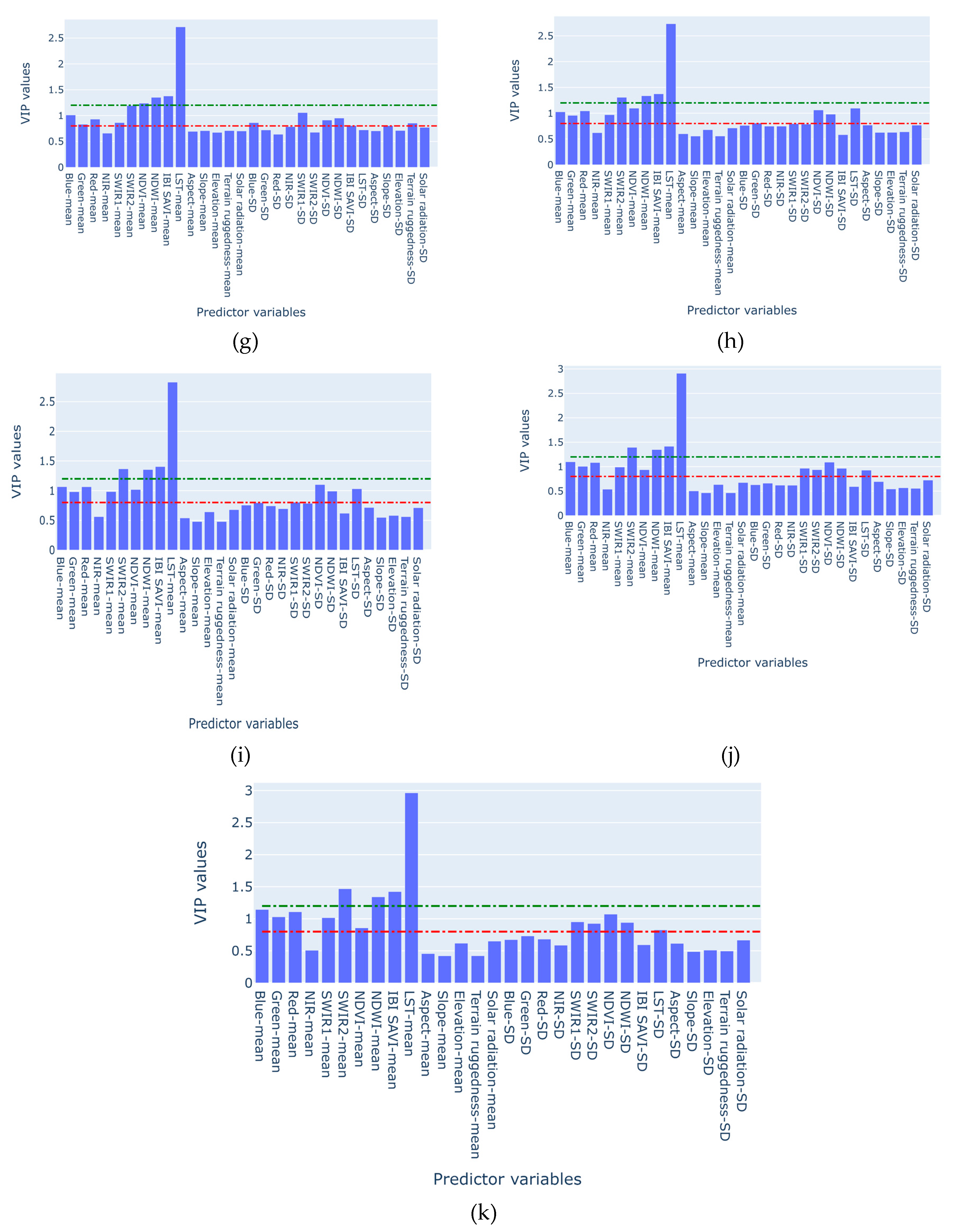
The estimated importance of the 30 predictor variables in the PLS regression model for all the sized buffer zones is shown in the Figure 3.
As mentioned above the selection of the sizes were stopped on the 1000m because the further increase of the radius results in an overlap of the areas between two weather stations.
As seen in Table 3 the number of VIP components varies over increasing the radius of the circles around the weather stations. The table x shows that the quantity of the components (predictor variables) stabilized.
The VIP scores for the 1000m buffer zone are shown in Table 4. LST-mean has the highest VIP score (2.77). According to table X the following variables have VIP scores greater than 1 (one): SWIR2_mean (1.42), IBI SAVI-mean (1.29) NDWI-mean (1.23). Blue-mean, red-mean and SWIR1_mean show scores of approximately 1.1 and NDVI_SD has a VIP score of 1.0. All the others are close to or below 1.
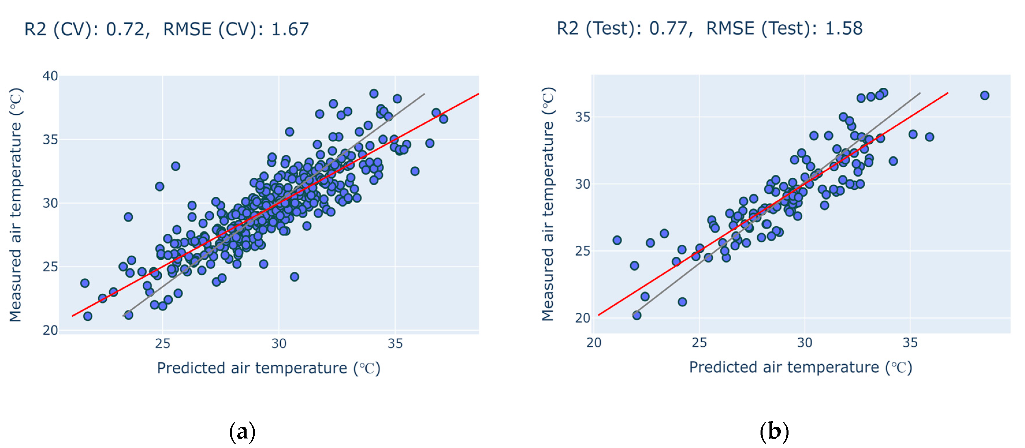
The results of the PLSR model received for 1000m buffer zone are shown in Figure 4. As it can be seen, the PLSR model provides satisfactory results both for calibration (R2Cal = 0.72, RMSECal = 1.67) and validation (R2Val = 0.77, RMSEVal = 1.58).
In this work, using PLSR driven by a wide range of predictor variables (30) values of Tair on an area with complex terrain features such as Yerevan (Armenia) have been predicted with high accuracy of RMSEVal =1.58 C. In the process, it was noticed that 5 predictor variables of the selected 10 with the high VIP scores also feature comparatively high (LST-mean: r=0.79; p<0.001) correlation coefficients (IBI-SAVI-mean: r=0.35; p<0.001 and SWIR2-mean; SWIR1-mean & Red-mean: r≈0.3; p<0.001). However, this shows that among these 5 variables Landsat-derived land surface temperature plays a key role in modeling Tair, with all other variables having a significantly smaller impact. The studies of Otgonbayar et al, concluded that PLSR represents well even seasonal and spatial variations in Tair when time-series of LST were included as predictor variables [21].
The results of the importance analysis highlighted a pool of parameters, which impact the most on Tair. The heterogeneity of the area makes it particularly difficult to venture guesses on the reasons for the composition of such pool of variables.
Previous studies on estimating urban Tair from remote sensing data were performed using more advanced ML models such as Random Forest, Cubist, Support Vector Machine (SVM), and neural networks to estimate urban air temperature [12,15,43]. Though we saw the great potential of the remote sensing data to estimate the Tair on Yerevan’s territory there is still a strong need to continue the studies using above-mentioned advanced ML models.

5. Conclusion

The main purpose of the research described in this paper was to assess the feasibility of estimating urban Tair, in a complex terrain configuration, based on remote sensing data alone using the PLRS model with a high amount of input variables. The novelty of this study includes the features of the considered area, complex and with a broad distribution of different elevations, and the high number of environmental parameters considered, exceeding 30. The key findings are outlined below:
  • Of the 30 parameters considered, 10 can be identified as relevant and can be used alone in the prediction; adding more parameters won’t improve prediction, but will require more computational resources;
  • the relevant parameters include a newly proposed modification of index IBI-SAVI, which turned out to be strongly impacting on Tair prediction;
  • Cross-validation analysis on temperature predictions across a station-centered 1000m circular area revealed quite a high correlation (R2Val = 0.77, RMSEVal = 1.58) between predicted and measured Tair from the test set;
  • In light of the above, we may estimate that remote sensing is an effective tool to estimate Tair distribution where a dense network of weather stations is not available.
Future developments will include incorporation of additional weather parameters from the weather stations such as precipitation and wind speed, and the use of non-parametric Machine Learning (ML) techniques, whose structure may be more suitable to represent the complex link between observables and target parameters in a complex environment like the one considered in this study.

Author Contributions

Conceptualization, S.A., G.T. V.M. and F.D. Methodology, S.A., G.T. V.M. and F.D. Data analysis and visualization, G.T., R.M., A.K. and A.H, Writing—review and editing, S.A., V.M., G.A. and F.D. All authors have read and agreed to the published version of the manuscript.

Funding

The work was supported by the Science Committee of the Ministry of Education Science Culture and Sport of RA, in the frames of the research project № 20TTCG-1E009.

Data Availability Statement

N/A.

Acknowledgments

The authors would like to acknowledge Department of GIS and Remote Sensing of the Center for Ecological-Noosphere Studies of the National Academy of Sciences (Armenia) and for the existing facilities to conduct this research and to the Department of Electrical, Computer and Biomedical Engineering, University of Pavia and in particular Dr. Fabio Dell’Aqua for the dedicated collaboration on the exchange of the experience when conducting the research and for support when preparing the manuscript. This study was fully supported by the Science Committee of the Ministry of education, science, sport and culture of RA in the frames of the research project № 20TTCG-1E009.

Conflicts of Interest

The authors declare no conflict of interest.

References

  1. Meliho, M.; Khattabi, A.; Zejli, D.; Orlando, C.A.; Dansou, C.E. Artificial Intelligence and Remote Sensing for Spatial Prediction of Daily Air Temperature: Case Study of Souss Watershed of Morocco. Geo-spatial Information Science 2022, 25, 244–258. [Google Scholar] [CrossRef]
  2. Ding, L.; Zhou, J.; Zhang, X.; Liu, S.; Cao, R. Downscaling of Surface Air Temperature over the Tibetan Plateau Based on DEM. International Journal of Applied Earth Observation and Geoinformation 2018, 73, 136–147. [Google Scholar] [CrossRef]
  3. Shah, D.B.; Pandya, M.R.; Trivedi, H.J.; Jani, A.R. Estimating Minimum and Maximum Air Temperature Using MODIS Data over Indo-Gangetic Plain. J Earth Syst Sci 2013, 122, 1593–1605. [Google Scholar] [CrossRef]
  4. Nichol, J.E.; To, P.H. Temporal Characteristics of Thermal Satellite Images for Urban Heat Stress and Heat Island Mapping. ISPRS Journal of Photogrammetry and Remote Sensing 2012, 74, 153–162. [Google Scholar] [CrossRef]
  5. Fu, P.; Weng, Q. Variability in Annual Temperature Cycle in the Urban Areas of the United States as Revealed by MODIS Imagery. ISPRS Journal of Photogrammetry and Remote Sensing 2018, 146, 65–73. [Google Scholar] [CrossRef]
  6. Vogt, J.V.; Viau, A.A.; Paquet, F. Mapping Regional Air Temperature Fields Using Satellite-Derived Surface Skin Temperatures. Int. J. Climatol. 1997, 17, 1559–1579. [Google Scholar] [CrossRef]
  7. Zakšek, K.; Schroedter-Homscheidt, M. Parameterization of Air Temperature in High Temporal and Spatial Resolution from a Combination of the SEVIRI and MODIS Instruments. ISPRS Journal of Photogrammetry and Remote Sensing 2009, 64, 414–421. [Google Scholar] [CrossRef]
  8. Cristóbal, J.; Ninyerola, M.; Pons, X. Modeling Air Temperature through a Combination of Remote Sensing and GIS Data. J. Geophys. Res. 2008, 113, D13106. [Google Scholar] [CrossRef]
  9. Mutiibwa, D.; Strachan, S.; Albright, T. Land Surface Temperature and Surface Air Temperature in Complex Terrain. IEEE J. Sel. Top. Appl. Earth Observations Remote Sensing 2015, 8, 4762–4774. [Google Scholar] [CrossRef]
  10. Nikoloudakis, N.; Stagakis, S.; Mitraka, Z.; Kamarianakis, Y.; Chrysoulakis, N. Spatial Interpolation of Urban Air Temperatures Using Satellite-Derived Predictors. Theor Appl Climatol 2020, 141, 657–672. [Google Scholar] [CrossRef]
  11. Orellana-Samaniego, M.L.; Ballari, D.; Guzman, P.; Ospina, J.E. Estimating Monthly Air Temperature Using Remote Sensing on a Region with Highly Variable Topography and Scarce Monitoring in the Southern Ecuadorian Andes. Theor Appl Climatol 2021, 144, 949–966. [Google Scholar] [CrossRef]
  12. Yoo, C.; Im, J.; Park, S.; Quackenbush, L.J. Estimation of Daily Maximum and Minimum Air Temperatures in Urban Landscapes Using MODIS Time Series Satellite Data. ISPRS Journal of Photogrammetry and Remote Sensing 2018, 137, 149–162. [Google Scholar] [CrossRef]
  13. Cifuentes, J.; Marulanda, G.; Bello, A.; Reneses, J. Air Temperature Forecasting Using Machine Learning Techniques: A Review. Energies 2020, 13, 4215. [Google Scholar] [CrossRef]
  14. Bechtel, B.; Zakšek, K.; Oßenbrügge, J.; Kaveckis, G.; Böhner, J. Towards a Satellite Based Monitoring of Urban Air Temperatures. Sustainable Cities and Society 2017, 34, 22–31. [Google Scholar] [CrossRef]
  15. Ho, H.C.; Knudby, A.; Sirovyak, P.; Xu, Y.; Hodul, M.; Henderson, S.B. Mapping Maximum Urban Air Temperature on Hot Summer Days. Remote Sensing of Environment 2014, 154, 38–45. [Google Scholar] [CrossRef]
  16. I, A.; C, C.; M, S. Estimation of Air Temperatures for the Urban Agglomeration of Athens with the Use of Satellite Data. Geoinformatics & Geostatistics: An Overview 2016, 2016. [Google Scholar] [CrossRef]
  17. Ho, H.C.; Knudby, A.; Xu, Y.; Hodul, M.; Aminipouri, M. A Comparison of Urban Heat Islands Mapped Using Skin Temperature, Air Temperature, and Apparent Temperature (Humidex), for the Greater Vancouver Area. Science of The Total Environment 2016, 544, 929–938. [Google Scholar] [CrossRef] [PubMed]
  18. Meyer, H.; Pebesma, E. Predicting into Unknown Space? Estimating the Area of Applicability of Spatial Prediction Models. Methods in Ecology and Evolution 2021, 12, 1620–1633. [Google Scholar] [CrossRef]
  19. Xu, Y.; Shen, Y. Reconstruction of the Land Surface Temperature Time Series Using Harmonic Analysis. Computers & Geosciences 2013, 61, 126–132. [Google Scholar] [CrossRef]
  20. Noi, P.T.; Degener, J.; Kappas, M. Comparison of Multiple Linear Regression, Cubist Regression, and Random Forest Algorithms to Estimate Daily Air Surface Temperature from Dynamic Combinations of MODIS LST Data. Remote Sensing 2017, 9, 398. [Google Scholar] [CrossRef]
  21. Otgonbayar, M.; Atzberger, C.; Mattiuzzi, M.; Erdenedalai, A. Estimation of Climatologies of Average Monthly Air Temperature over Mongolia Using MODIS Land Surface Temperature (LST) Time Series and Machine Learning Techniques. Remote Sensing 2019, 11, 2588. [Google Scholar] [CrossRef]
  22. Wang, C.; Bi, X.; Luan, Q.; Li, Z. Estimation of Daily and Instantaneous Near-Surface Air Temperature from MODIS Data Using Machine Learning Methods in the Jingjinji Area of China. Remote Sensing 2022, 14, 1916. [Google Scholar] [CrossRef]
  23. Rasul, A.; Balzter, H.; Smith, C. Applying a Normalized Ratio Scale Technique to Assess Influences of Urban Expansion on Land Surface Temperature of the Semi-Arid City of Erbil. International Journal of Remote Sensing 2017, 38, 3960–3980. [Google Scholar] [CrossRef]
  24. Statistical Committee of the Republic of Armenia Available online:. Available online: https://www.armstat.am/en/ (accessed on 13 March 2023).
  25. Yerevan Green City Action Plan Available online:. Available online: https://www.yerevan.am/en/yerevan-green-city-action-plan/ (accessed on 13 March 2023).
  26. Tepanosyan, G.; Muradyan, V.; Hovsepyan, A.; Pinigin, G.; Medvedev, A.; Asmaryan, S. Studying Spatial-Temporal Changes and Relationship of Land Cover and Surface Urban Heat Island Derived through Remote Sensing in Yerevan, Armenia. Building and Environment 2021, 187, 107390. [Google Scholar] [CrossRef]
  27. Climate Change Information Center Available online:. Available online: http://www.nature-ic.am/en (accessed on 13 March 2023).
  28. Third National Communication on Climate Change: Under the United Nations Framework Convention on Climate Change. Yerevan..; 2015;
  29. Foga, S.; Scaramuzza, P.L.; Guo, S.; Zhu, Z.; Dilley, R.D.; Beckmann, T.; Schmidt, G.L.; Dwyer, J.L.; Joseph Hughes, M.; Laue, B. Cloud Detection Algorithm Comparison and Validation for Operational Landsat Data Products. Remote Sensing of Environment 2017, 194, 379–390. [Google Scholar] [CrossRef]
  30. Xu, H. A New Index for Delineating Built-up Land Features in Satellite Imagery. International Journal of Remote Sensing 2008, 29, 4269–4276. [Google Scholar] [CrossRef]
  31. Parastatidis, D.; Mitraka, Z.; Chrysoulakis, N.; Abrams, M. Online Global Land Surface Temperature Estimation from Landsat. Remote Sensing 2017, 9, 1208. [Google Scholar] [CrossRef]
  32. Jimenez-Munoz, J.C.; Cristobal, J.; Sobrino, J.A.; Soria, G.; Ninyerola, M.; Pons, X.; Pons, X. Revision of the Single-Channel Algorithm for Land Surface Temperature Retrieval From Landsat Thermal-Infrared Data. IEEE Trans. Geosci. Remote Sensing 2009, 47, 339–349. [Google Scholar] [CrossRef]
  33. Jimenez-Munoz, J.C.; Sobrino, J.A.; Skokovic, D.; Mattar, C.; Cristobal, J. Land Surface Temperature Retrieval Methods From Landsat-8 Thermal Infrared Sensor Data. IEEE Geosci. Remote Sensing Lett. 2014, 11, 1840–1843. [Google Scholar] [CrossRef]
  34. Riley, S.; Degloria, S.; Elliot, S.D. A Terrain Ruggedness Index That Quantifies Topographic Heterogeneity. Internation Journal of Science 1999, 5, 23–27. [Google Scholar]
  35. Chuai, X.W.; Huang, X.J.; Wang, W.J.; Bao, G. NDVI, Temperature and Precipitation Changes and Their Relationships with Different Vegetation Types during 1998–2007 in Inner Mongolia, China. International Journal of Climatology 2013, 33, 1696–1706. [Google Scholar] [CrossRef]
  36. Hou, G.; Zhang, H.; Wang, Y. Vegetation Dynamics and Its Relationship with Climatic Factors in the Changbai Mountain Natural Reserve. J. Mt. Sci. 2011, 8, 865–875. [Google Scholar] [CrossRef]
  37. Yagoub, Y.E.; Li, Z.; Musa, O.S.; Anjum, M.N.; Wang, F.; Bi, Y.; Zhang, B. Correlation between Climate Factors and Vegetation Cover in Qinghai Province, China. Journal of Geographic Information System 2017, 9, 403–419. [Google Scholar] [CrossRef]
  38. Zhao, Z.-Q.; He, B.-J.; Li, L.-G.; Wang, H.-B.; Darko, A. Profile and Concentric Zonal Analysis of Relationships between Land Use/Land Cover and Land Surface Temperature: Case Study of Shenyang, China. Energy and Buildings 2017, 155, 282–295. [Google Scholar] [CrossRef]
  39. Cui, L.; Shi, J. Temporal and Spatial Response of Vegetation NDVI to Temperature and Precipitation in Eastern China. J. Geogr. Sci. 2010, 20, 163–176. [Google Scholar] [CrossRef]
  40. Gitelson, A.A.; Kaufman, Y.J. MODIS NDVI Optimization To Fit the AVHRR Data Series—Spectral Considerations. Remote Sensing of Environment 1998, 66, 343–350. [Google Scholar] [CrossRef]
  41. Pedregosa, F.; Varoquaux, G.; Gramfort, A.; Michel, V.; Thirion, B.; Grisel, O.; Blondel, M.; Prettenhofer, P.; Weiss, R.; Dubourg, V.; et al. Scikit-Learn: Machine Learning in Python. Journal of Machine Learning Research 2012, 12. [Google Scholar]
  42. Zakharov, V.P.; Bratchenko, I.A.; Artemyev, D.N.; Myakinin, O.O.; Kozlov, S.V.; Moryatov, A.A.; Orlov, A.E. 17-Multimodal Optical Biopsy and Imaging of Skin Cancer. In Neurophotonics and Biomedical Spectroscopy; Elsevier, 2019; pp. 449–476. ISBN 978-0-323-48067-3. [Google Scholar]
  43. Zhang, H.; Zhang, F.; Ye, M.; Che, T.; Zhang, G. Estimating Daily Air Temperatures over the Tibetan Plateau by Dynamically Integrating MODIS LST Data. JGR Atmospheres 2016, 121. [Google Scholar] [CrossRef]
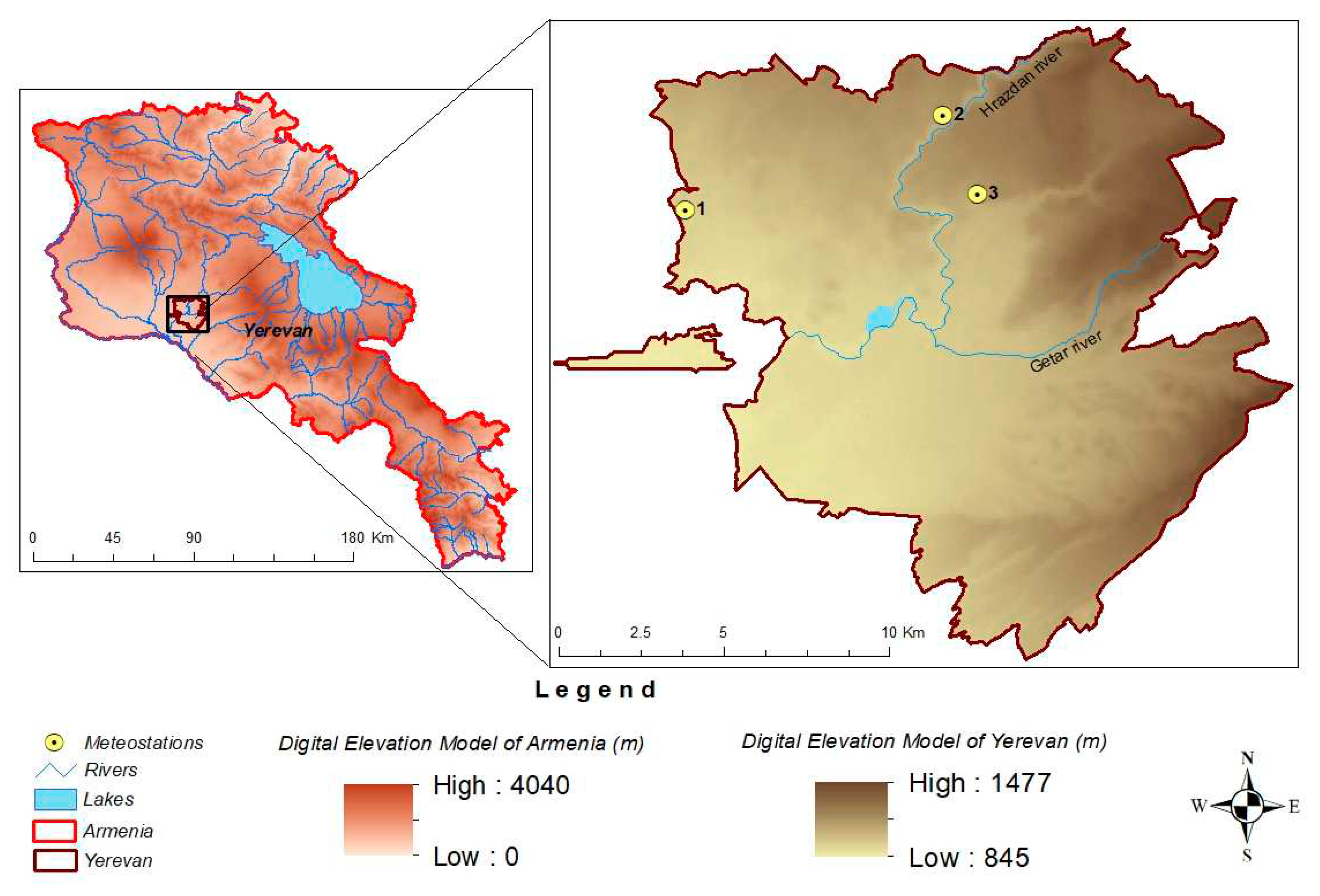
Figure 1. Geographical location and hypsometry of Armenia and Yerevan and the distribution of the weather stations on territory of Yerevan: 1. Yerevan_agro; 2. Yerevan_aerologia; 3.Arabkir.
Preprints 70437 g001
Figure 2. Methodological flowchart of the study.
Preprints 70437 g002
Figure 3. PLSR variable importance for each circled zone: a) 30m; b) 100m; c) 200m; d) 300m; e) 400m; f) 500m; g) 600m; h) 700m; i) 800m; j) 900m; k) 1000m.
Preprints 70437 g003aPreprints 70437 g003b
Figure 4. Scatter plot of predicted vs. measured Tair contents when validating the PLSR model: a. cross validation; b. testing.
Preprints 70437 g004
Table 1. Geographical coordinates and altitude of the weather stations operating on the territory of Yerevan.
N Name of station Latitude Longitude Height a. s. l. (m)
1. Yerevan_agro 40°11’19” N 44°23’55’’ E 942
2. Yerevan_aerologia 40°13’2” N 44°29’59’’ E 1134
3. Arabkir 40°11’43” N 44°30’44’’ E 1113
Table 2. Pearson correlations between Tair and all components.
N Variables Correlation coefficient (r) p_value
1. Blue_mean 0.1374137 2.0728e-3
2. Green_mean 0.1564202 4.472e-4
3. Red_mean 0.2612906 3.004e-9
4. NIR_mean 0.0125771 7.790636e-1
5. SWIR1_mean 0.2861474 7.066e-11
6. SWIR2_mean 0.2990162 8.715e-12
7. NDVI_mean -0.252406 1.048e-8
8. NDWI_mean -0.3451834 1.946e-15
9. IBI SAVI_mean 0.348421 1.022E-15
10. LST_mean 0.7921705 1.022e-15
11. Aspect_mean -0.0700592 1.176829e-1
12. Slope_mean -0.0632945 1.576022e-1
13. Elev_mean -0.0810757 7.00863e-2
14. Rugged_mean -0.0616125 1.689591e-1
15. Sol_rad_mean -0.1930203 1.385e-5
16. Blue_SD -0.0980034 2.84362e-2
17. Green_SD -0.0927548 3.81405e-2
18. Red_SD -0.0702113 1.16886e-1
19. NIR_SD -0.0703557 1.161338e-1
20. SWIR1_SD -0.0904733 4.3163e-2
21. SWIR2_SD -0.1321922 3.0613e-3
22. NDVI_SD -0.2639066 2.061e-9
23. NDWI_SD -0.2410586 4.831e-8
24. IBI SAVI_SD -0.1247979 5.1978e-3
25. LST_SD -0.0077571 8.626332e-1
26. Aspect_SD 0.1097252 1.40961e-2
27. Slope_SD -0.0265121 5.542198e-1
28. Elev_SD -0.0986305 2.74328e-2
29. Rugged_SD -0.022174 6.208505e-1
30. Sol_rad_SD 0.0385449 3.897596e-1
Table 3. The PLSR descriptive for the different sized areas with VIP scores.
PLSR
descriptive
30 m 100 m 200 m 300 m 400 m 500 m 600 m 700 m 800 m 900 m 1000 m
R2Train 0.72 0.73 0.73 0.75 0.75 0.74 0.75 0.75 0.75 0.76 0.76
RMSETrain 1.68 1.66 1.65 1.58 1.58 1.61 1.60 1.59 1.59 1.57 1.56
R2CV 0.68 0.68 0.68 0.71 0.71 0.70 0.71 0.70 0.70 0.71 0.72
RMSECV 1.80 1.79 1.80 1.70 1.70 1.73 1.73 1.74 1.74 1.71 1.67
R2Test 0.70 0.71 0.71 0.73 0.72 0.73 0.72 0.74 0.74 0.75 0.77
RMSETest 1.78 1.73 1.75 1.69 1.71 1.69 1.72 1.65 1.65 1.61 1.58
N of VIP
components
14 14 10 14 14 13 14 10 10 10 10
Table 4. The list of the variables with VIP scores.
N Predictor variables VIP scores
1. Blue-mean 1.112
2. Green-mean 1.018
3. Red-mean 1.098
4. NIR-mean 0.682
5. SWIR1-mean 1.066
6. SWIR2-mean 1.414
7. NDVI-mean 0.898
8. NDWI-mean 1.224
9. IBI SAVI-mean 1.285
10. LST-mean 2.772
11. Aspect-mean 0.660
12. Slope-mean 0.667
13. Elevation-mean 0.642
14. Terrain ruggedness-mean 0.666
15. Solar radiation-mean 0.661
16. Blue-SD 0.729
17. Green-SD 0.691
18. Red-SD 0.658
19. NIR-SD 0.712
20. SWIR1-SD 0.909
21. SWIR2-SD 0.894
22. NDVI-SD 1.011
23. NDWI-SD 0.922
24. IBI SAVI-SD 0.585
25. LST-SD 0.959
26. Aspect-SD 0.745
27. Slope-SD 0.650
28. Elevation-SD 0.710
29. Terrain ruggedness-SD 0.649
30. Solar radiation-SD 0.687
Disclaimer/Publisher’s Note: The statements, opinions and data contained in all publications are solely those of the individual author(s) and contributor(s) and not of MDPI and/or the editor(s). MDPI and/or the editor(s) disclaim responsibility for any injury to people or property resulting from any ideas, methods, instructions or products referred to in the content.
Copyright: This open access article is published under a Creative Commons CC BY 4.0 license, which permit the free download, distribution, and reuse, provided that the author and preprint are cited in any reuse.
Prerpints.org logo

Preprints.org is a free preprint server supported by MDPI in Basel, Switzerland.

Subscribe

© 2024 MDPI (Basel, Switzerland) unless otherwise stated