Assessing the Feasibility of Wave Energy Harvesting through Coastal Wave Modeling and Forecasting with Long Short-Term Memory Optimization using Univariate Time Series Approach

1. Introduction

Coastal wave modeling has improved significantly in recent decades, due to the emergence of artificial intelligence applications. However, they still have a long way to go. Such modeling has a wide range of applications in fishing, maritime transport, naval navigation, environmental research, risk management and sustainable energy [1,2]. The advancement of activities in both nearshore and offshore waters requires knowledge of the wave condition [3,4] and the need to develop state-of-art wave forecasting systems. The wave prediction models are essential for disaster prevention and preparedness, optimization of shipping routes, climate change awareness, and ocean power generation [5]. Many research work has been done in the domain of coastal wave modeling, and the researchers have made a great breakthrough in forecasting wave conditions. However, wave predictions are sometimes inaccurate.

The wave modeling is frequently applied to simulate the significant physical occurrence in the coastal area [6,7]. For modeling and forecasting wave conditions, there is a need to consider and understand features like direction, frequency, speed, timing of waves, pressure, and wave height (amplitude), among others, and the correlation between these features. Different approaches are employed for coastal wave modeling [8,9,10]. The three primary modeling methods used are physical, numerical, and composite. Numerical models (NM) refer to the usage of computer codes (commercial, open source, or home-produced software) [11], and physical models (PM) refer to the usage of laboratory models at a suitable scale (micro, small, medium, and large-scale models) to study the process of interest, while composite models (CM) refer to the combined and proportional use of physical and numerical models [12]. At this phase, the conventional method of forecasting waves by oceanographers is numerical models [6]. To solve complex equations, the numerical models use various oceanic features as inputs, such as direction, speed, height, temperature, and pressure.

The most commonly used models nowadays are Simulating Waves Nearshore (SWAN) [6,7,8,9,10,11,12,13], which the Delft University of Technology developed and introduced by Booij et al. in 1999 [14], and WaveWatch III (WW3) was introduced by Tolman et al. in 2009 [15]. WaveWatch III (WW3) is a third-generation wave model developed by National Oceanic and Atmospheric Administration (NOAA)/ National Centers for Environmental Prediction (NCEP) [16].

The advantages of physical simulation and data-driven techniques are combined in traditional numerical model forecasting techniques to produce high spatial and sequential resolution predictions [17,18]. However, it has substantial drawbacks in real-world offshore sector applications because the accuracy and time lag are not guaranteed. Additionally, the numerical model should be carefully considered as an operational application due to the high computational and maintenance expenses [19,20,21].

Machine learning techniques have increasingly incorporated ocean wave prediction due to their advantages in establishing nonlinear mapping relationships, which can significantly boost prediction accuracy [22]. By combining the correlations between wind and wind waves with the data produced by a numerical model, Song et al. [6] developed a hybrid method called ConvLSTM by coupling CNN with LSTM to improve the predictions of significant height Berbić et al. [23] use two classification models, ANN, and support vector machine (SVM), for significant wave height prediction.

Barbara et al. [24] use artificial neural networks (ANN) to forecast wave reflection from coastal and harbor structures. The network's accuracy is quite good, with an average root mean squared error of less than 0.04. Elbisy et al. [25] developed a model using SVM with a genetic algorithm to predict wave direction and height and compare it with a neural network. The findings of this study show that the SVM model (RBF kernel) is a suitable alternative to NN for predicting wave parameters.

Even though the use of AI in wave condition forecasting is becoming increasingly common [6], most of them have concentrated on wave height and other wave characteristics employing classification techniques like ANN and time series approaches like CNN (Covn1D), GRU, and LSTM.

Forecasting wave speed and direction is critical in marine energy harvesting because of the significant impact of these elements [26]. Most of the literature we found in various academic databases does not explicitly apply univariate or multivariate time series approaches to forecast these wave characteristics.

Wave energy harvesting uses the energy of ocean or sea waves to generate electricity, and the direction and speed of the waves play a significant role in the efficiency of this process [27]. The orientation of wave energy devices, such as wave energy converters or wave farms, can be determined by the waves' direction, and the speed of the waves can affect the amount of energy that can be generated [28,29]. It is possible to optimize the location and operation of wave energy devices to maximize their energy-generating capacity by forecasting the direction and speed of ocean waves [1,30]. In addition, accurate predictions of wave direction and speed can help limit the risk of infrastructure damage and safeguard the safety of employees working in wave energy operations [29,30,31].

As part of Brunei Darussalam's vision for 2035 and energy transition, the country plans to harness vast marine energy from the South China Sea and fulfill its net zero commitment. According to Brunei Darussalam 2012 report prepared by the United Nations Climate Technology Centre and Network (UNCTCN). Approximately 269 km of Brunei Darussalam's coastline has the capacity to generate between 15 and 126 GW of wave energy, with an annual theoretical potential of 66 x 1010 W [32]. This study aims to conduct a preliminary efficiency and feasibility assessment of wave energy harvesting in Brunei Darussalam waters in the South China Sea.

Although technologies currently exist to harness wave energy in coastal areas, the capital cost of wave farms can be high [29], so it is essential to model the power to be generated in advance. The two main objectives of this experiment are to use numerical models to simulate wave conditions. The second objective is to build a univariate time series forecasting model capable of predicting wave direction and speed using long short-term memory (LSTM) recurrent neural networks.

The rest of the paper is structured as follows: Section 2 presents the data used throughout the study, and explanatory data analysis. Section 3 describes the experimental method of the study. Section 4 illustrates and analyzes the experimental results with a discussion. Section 5 highlights the future research plan, and Section 6 presents the conclusion based on the study findings.

2. Study Data and Explanatory Data Analysis

2.1. Data

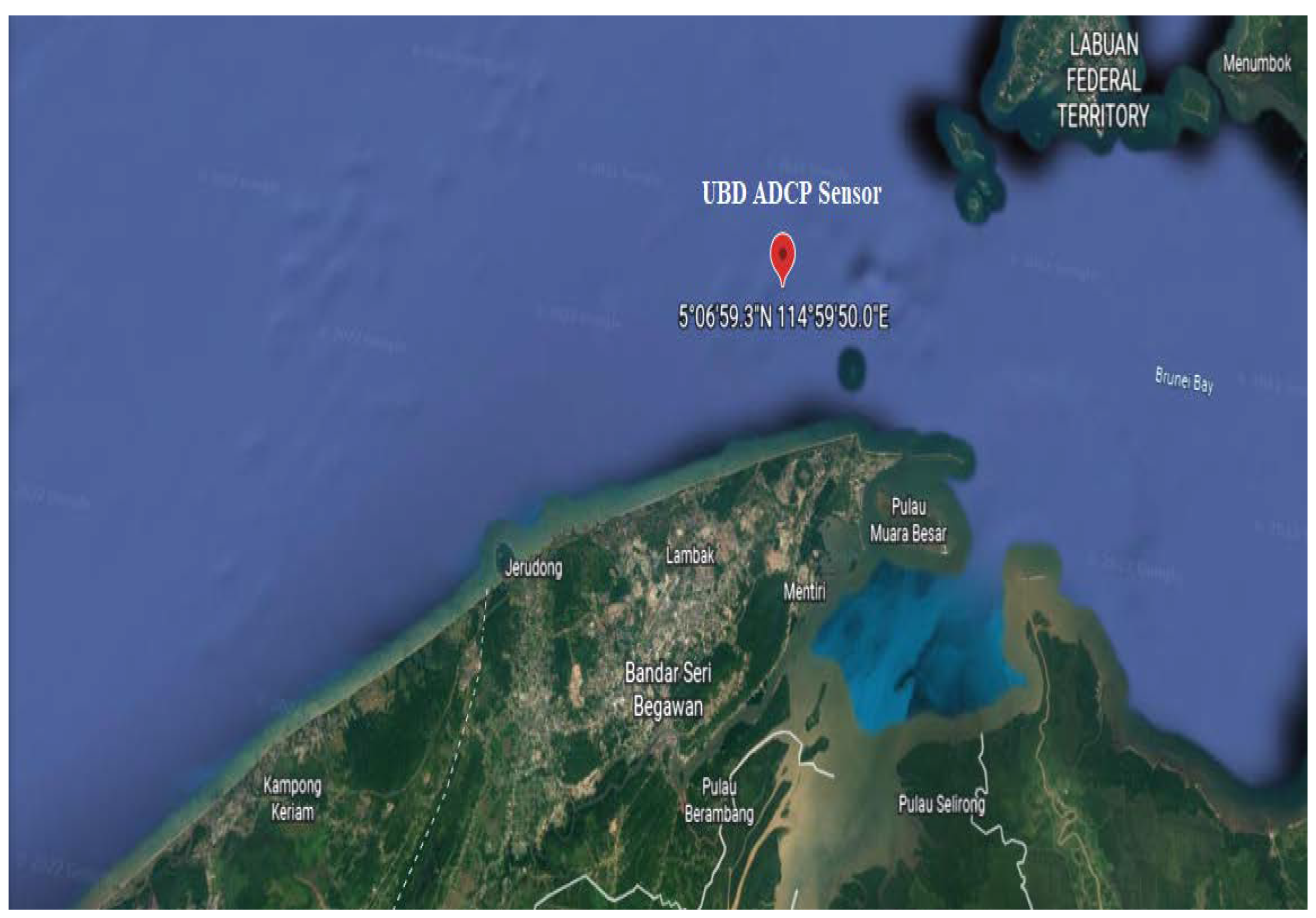
Data for this experiment was computed using a high-precision underwater Acoustic Doppler Current Profiler (ADCP) sensor data collected in the territorial waters of Brunei Darussalam. Along the South China Sea coast at coordinates GPS (05 06.988 N, 114 59.833 E), procured by Universiti Brunei Darussalam for research purposes. The raw data collected by the sensor consists of many wave condition parameters, including temperature, pressure, significant wave height (Hm0), frequency, and current speed, and direction of different depths. Initially, professional divers placed the ADCP sensor on the seabed for data collection. Later, the sensor was retaken, and the raw data was retrieved using AquaPro. This software can also be used to monitor the wave condition captured by the sensor in real-time. The raw data file can be obtained by connecting the ADCP sensor with AquaPro. The raw data file was then uploaded to Storm64 for data visualization and preprocessing. The processed wave elements datasets can be generated at this stage and exported in different file formats like csv, txt, Whr, etc. AquaPro and Storm64 are developed by the sensor manufacturer Nortek Group, Australia. The exported preprocessed dataset underwent a data cleaning process before use. The wave speed and direction were estimated using the processed data collected from the sensor.

Figure 1. Google map indicating the location of the ADCP sensor on the South China Sea.

Figure 1. Google map indicating the location of the ADCP sensor on the South China Sea.

2.2. Exploratory Data Analysis (EDA)

Exploratory data analysis (EDA) is an essential step in data analysis. Data are examined and summarized to gain insight into their characteristics, identify patterns and relationships, and uncover potential problems. The goal of EDA is to gain a deeper understanding of the data and select appropriate statistical models and techniques for subsequent analysis. EDA typically involves a combination of visual and numerical methods. Visual techniques include plotting time series data, histograms, boxplots, scatter plots, and heat maps to identify patterns, trends, seasonality, outliers, and correlations. Numerical techniques include calculating summary statistics such as mean, variance, standard deviation, skewness, and kurtosis to describe the distribution and shape of the data.

The following are the statistical tools that have been used in an EDA.

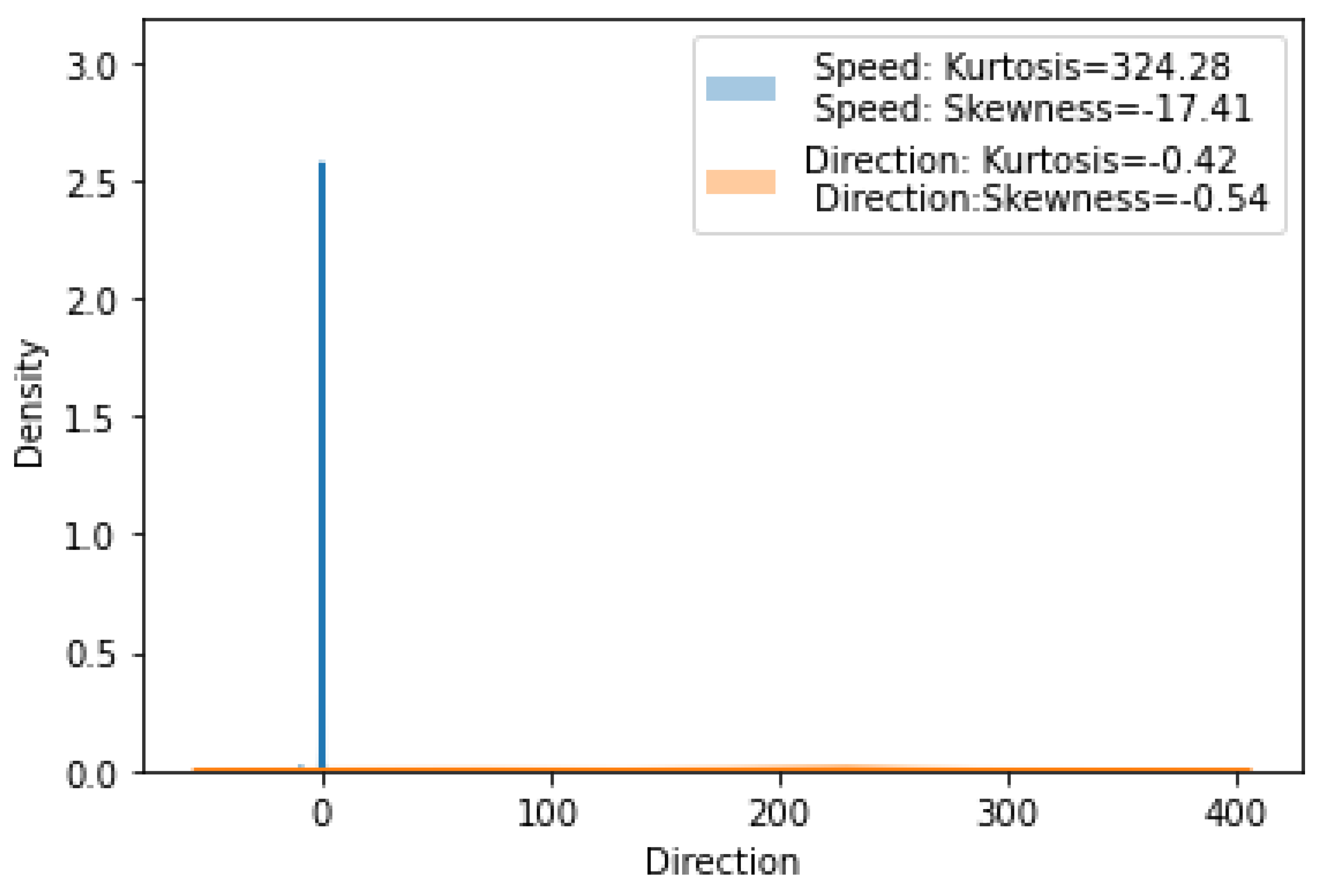
1. Kurtosis: In a distribution with high kurtosis, more values are concentrated around the mean, and the distribution's tails are fatter or more spread out. In a distribution with low kurtosis, fewer values are concentrated around the mean, and the tails are thinner or less widely spread. Figure 2 illustrates the kurtosis and skewness plot of the wave speed and direction and their values.

2. Skewness: in a positively skewed distribution, the tail is on the right side, and the mean is greater than the median. A negatively skewed distribution has a tail on the left side, and the mean is less than the median. Asymmetric distribution has no skewness. Histogram representation: A histogram can help identify the shape of a variable's distribution, such as whether it is symmetric, skewed, or bimodal. Figure 2 shows the kurtosis and skewness plot of the wave speed and direction and their values.

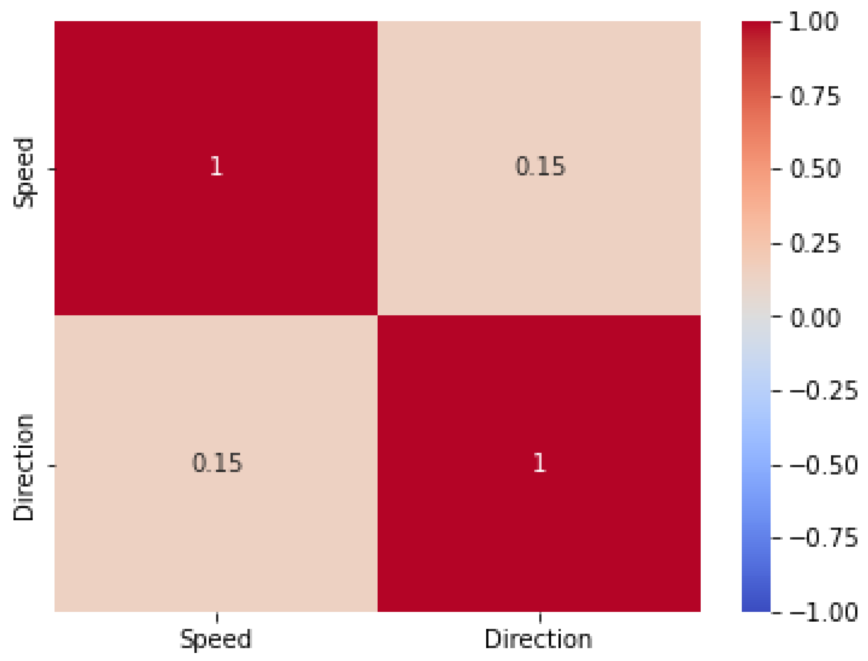
3. Correlation Heatmap: A correlation heatmap can help determine the strength and direction of the relationship between two or more variables. It can also help identify possible outliers or unusual observations. Figure 3 clearly illustrates the correlation heatmap between wave speed and direction.

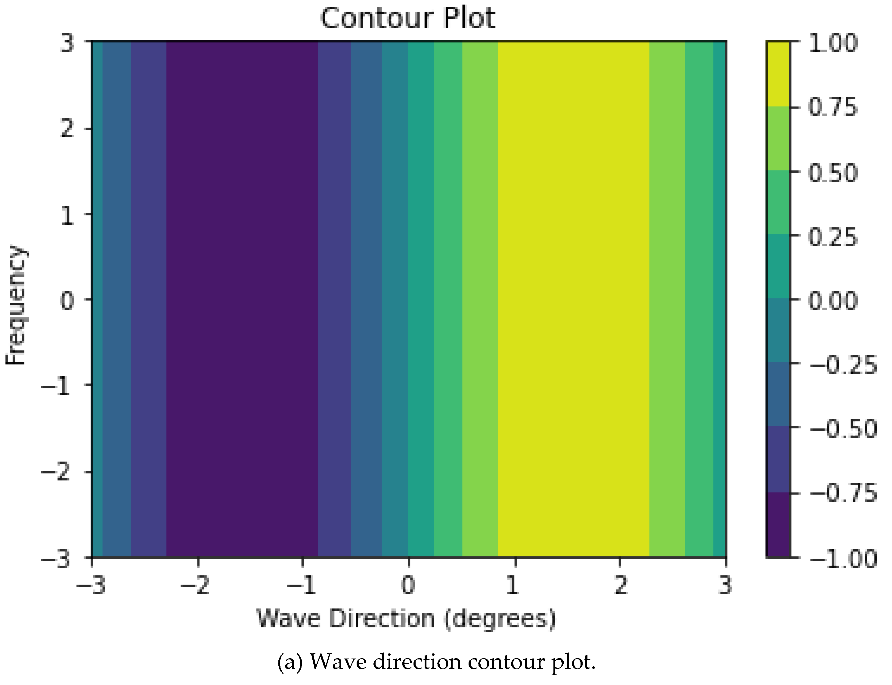
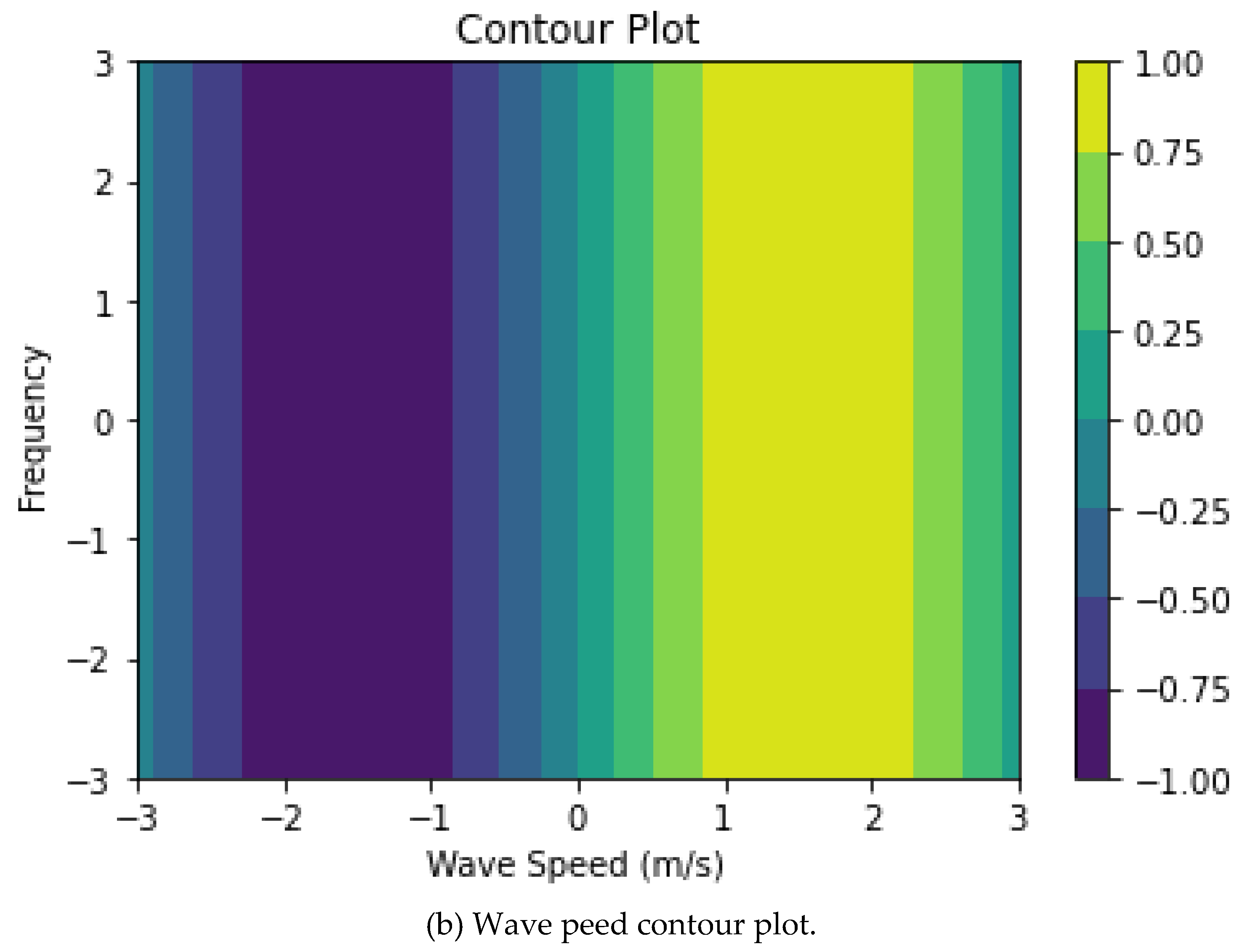
4. Contour plot: a contour plot can help visualize the relationship between two input variables and the output variable. The contour lines connect points with the same output value, so you can see how the output changes when the input variables change. Figure 4 display contour plots of wave speed and direction.

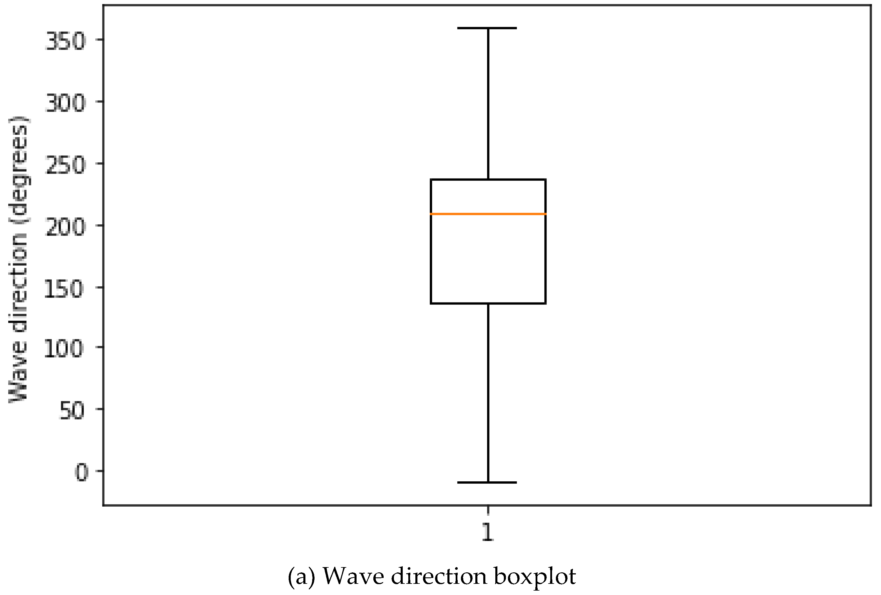
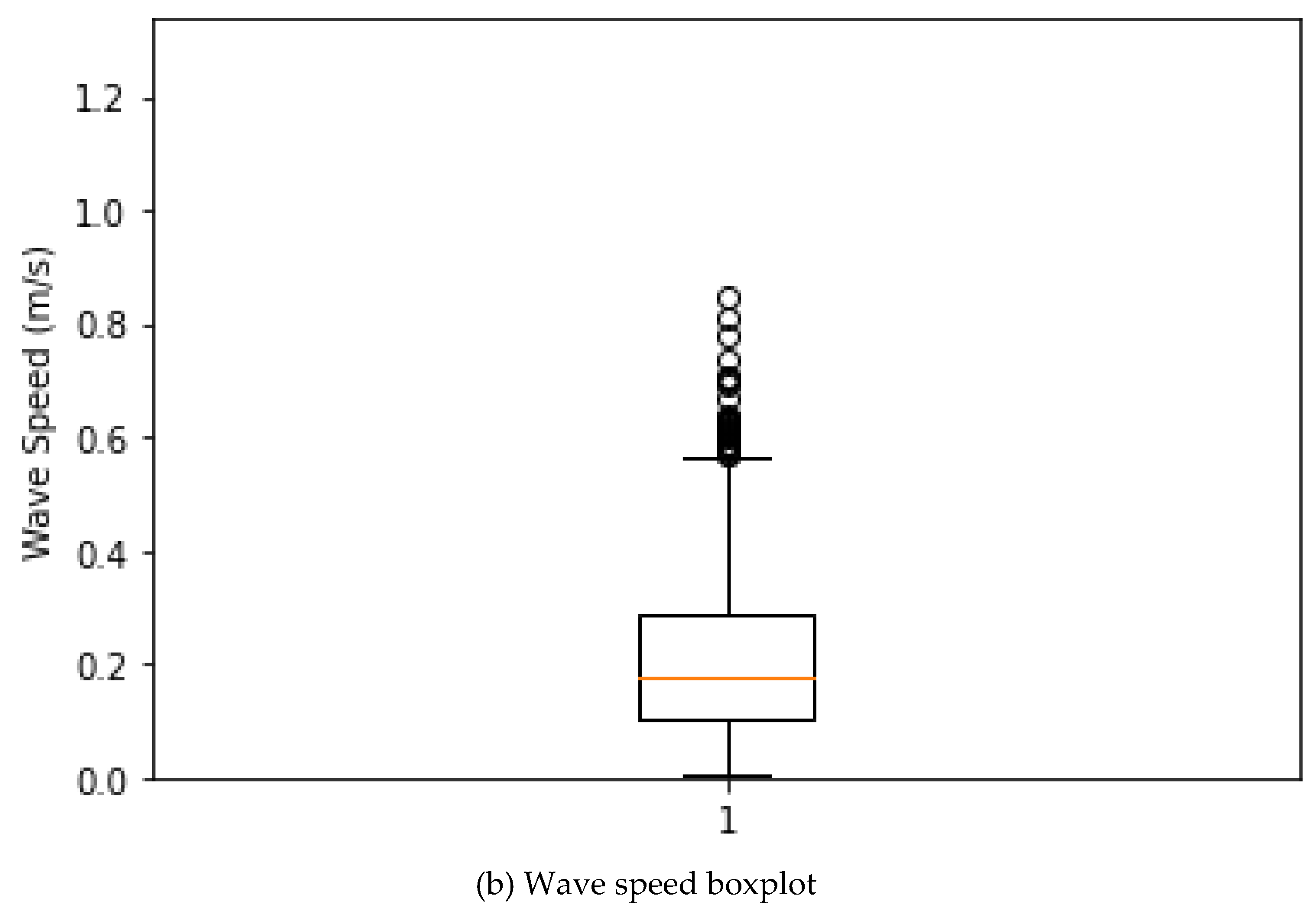
5. Box plot: A box plot can provide information about the distribution of a variable, including the median, quartiles, range, and any outliers. It can also help identify any skewness or asymmetry in the data. Figure 5 shows the boxplots of wave speed and direction.

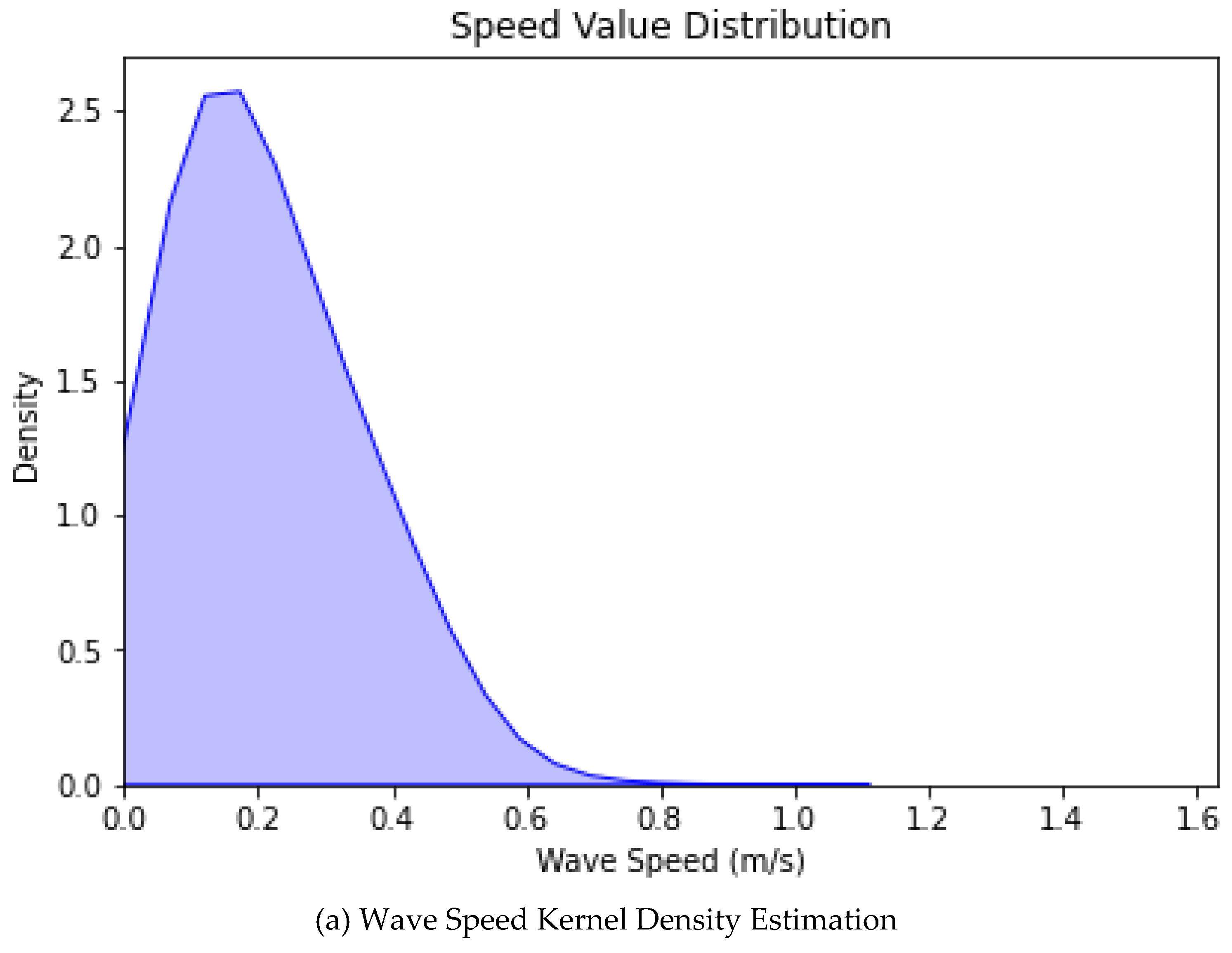
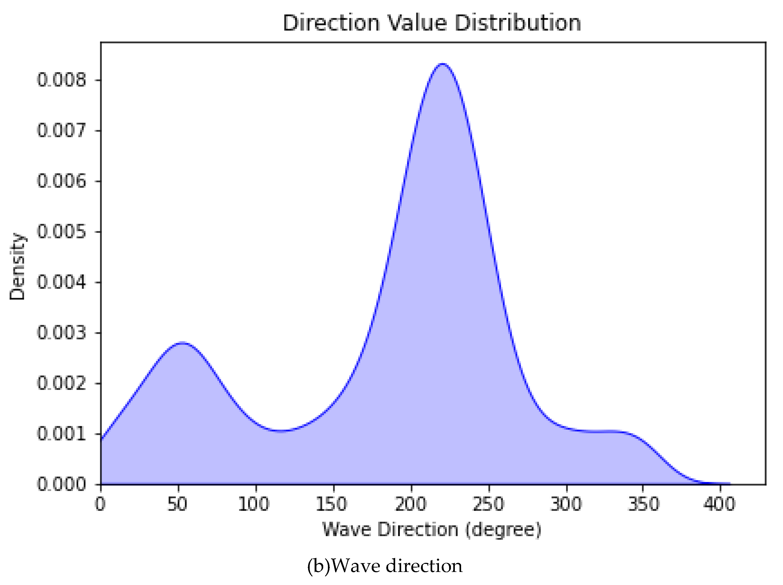
6. Kernel density estimation plot: A kernel density estimation plot can help determine the shape and spread of a distribution. It is instrumental when the underlying distribution is unknown or difficult to describe with a parametric model. It can also help identify possible multimodality in the data. In Figure 6, the kernel density plot (KDE) plots depicting wave speed and direction are presented.

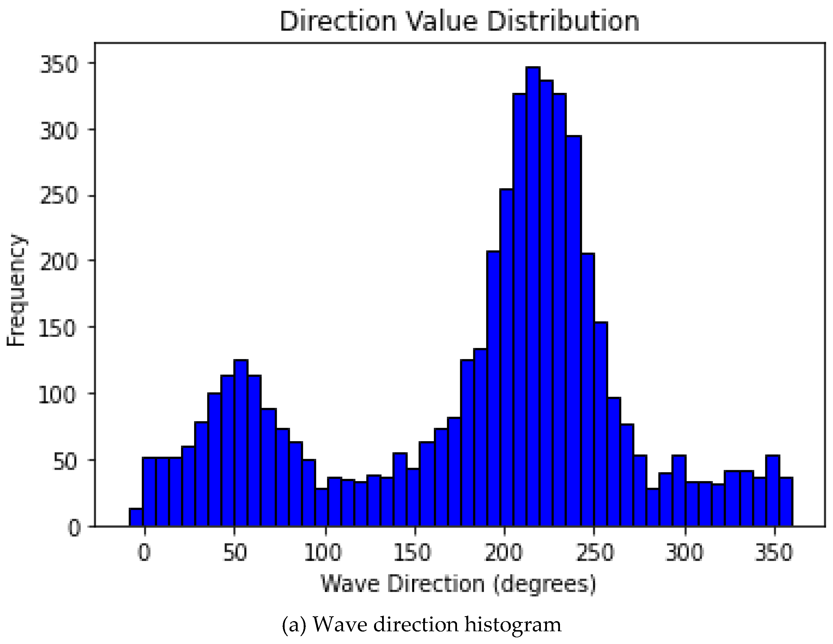
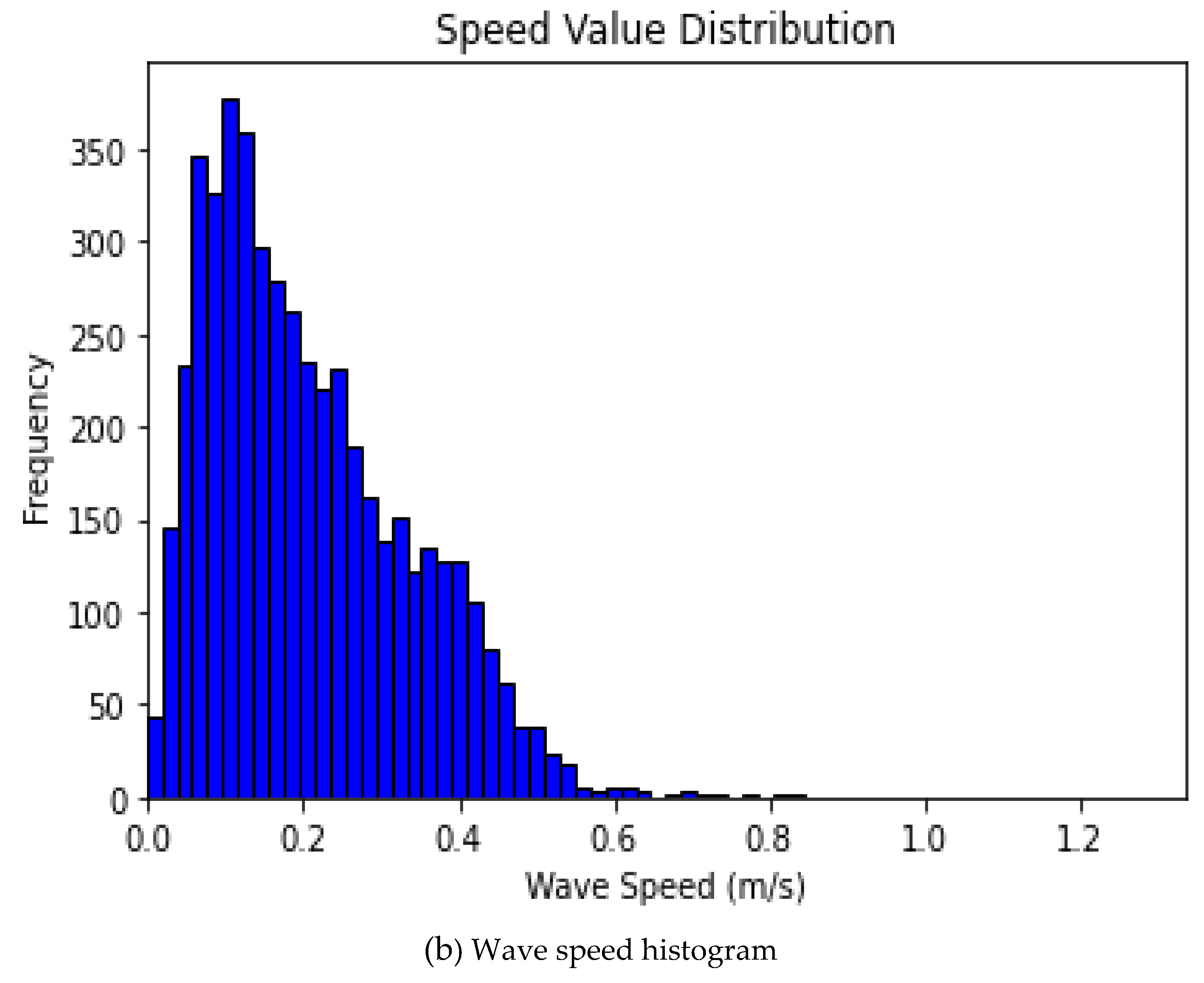
7. Histogram: A histogram is a graphical representation of the distribution of numerical data. It is an essential tool used in exploratory data analysis (EDA) to summarize the underlying distribution of a dataset. Figure 7 exhibits the histogram plots for both wave speed and direction.

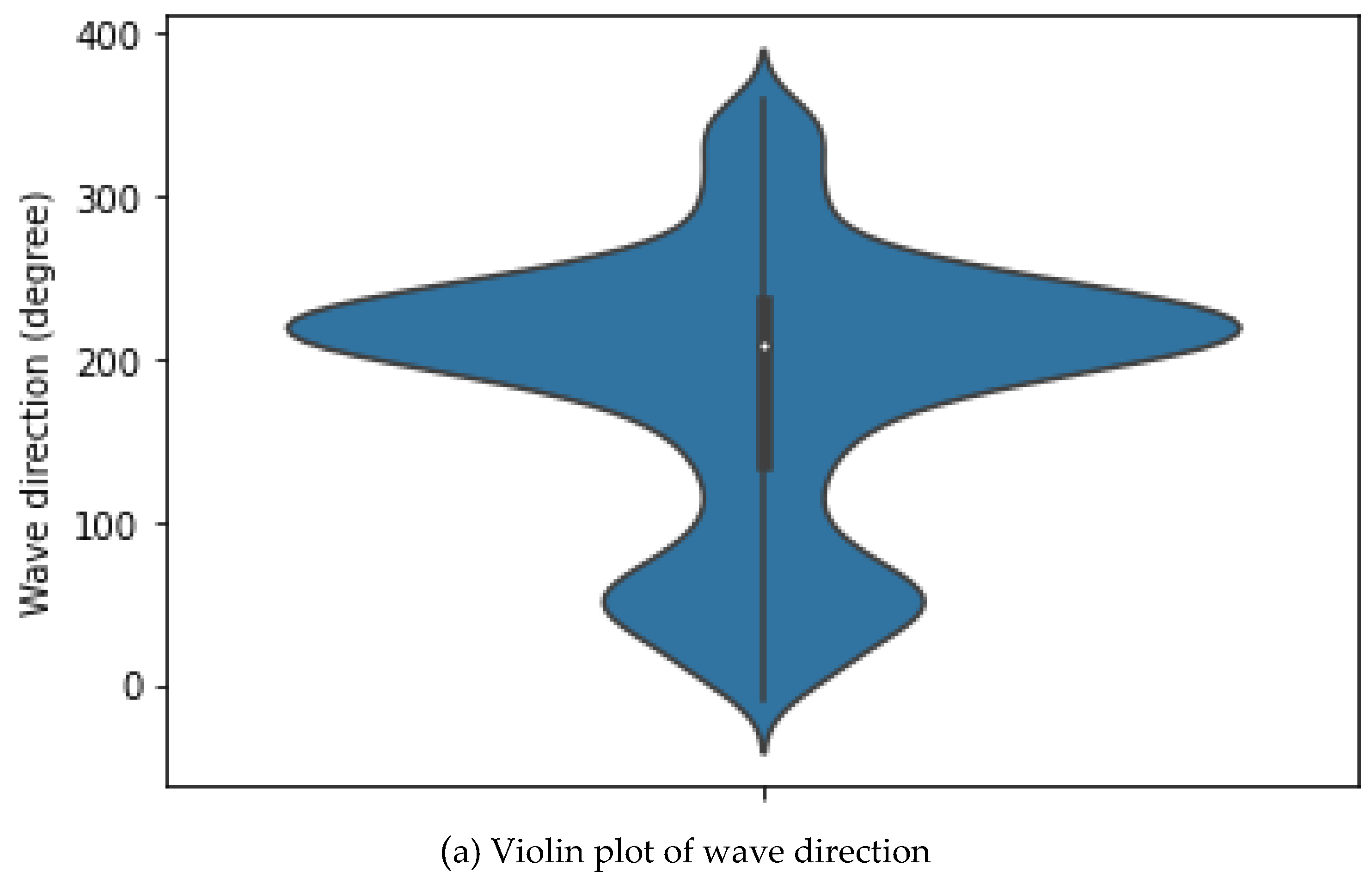
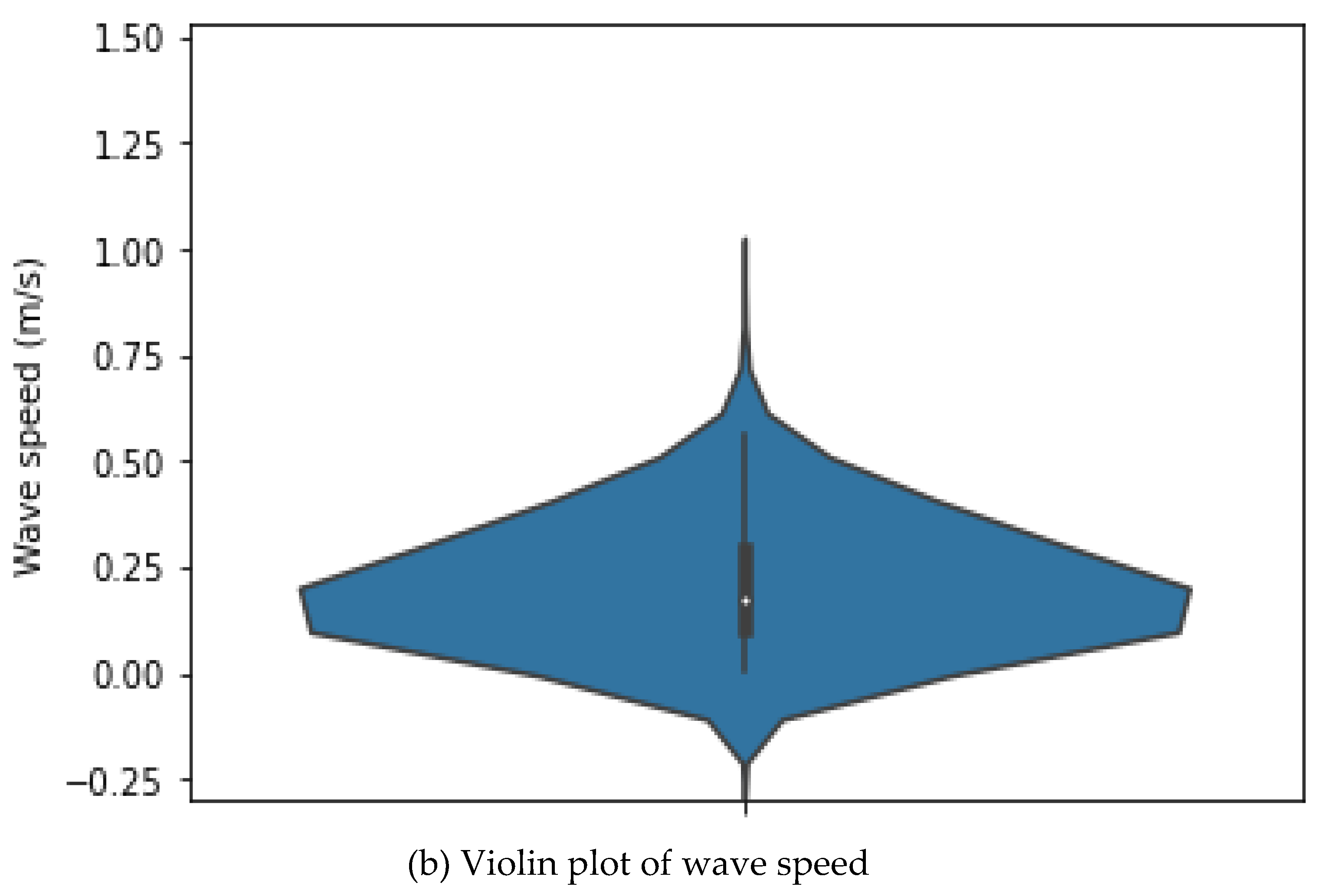
8. Violin plot: A violin plot is a plot that combines a boxplot with a kernel density estimation plot to show the distribution of a continuous variable. It has a wide "body" in the middle and narrow "tails" at the ends, with the width indicating the density of the data and the tail indicating the range. The boxplot within the violin plot shows the median, quartiles, and outliers. Violin plots are useful for comparing the distributions of multiple variables because they show summary statistics and the distribution shape in a single plot. Figure 8, illustrates the violin plots for both wave speed and direction.

3. Materials and Methods

The methodology in this experiment consists of two parts. The first subsection is the wave speed and direction simulation using numerical methods for modeling and simulation. In contrast, the second subsections contain the details of univariate time series optimization and forecast using KerasTuner with long-short term memory (LSTM).

3.1. Numerical modelling and simulation

Numerical methods are mathematical techniques used to approximate solutions to problems that are difficult or impossible to solve analytically [33,34,35]. One such problem is wave speed and direction simulation, which can be approximated using the finite difference method and the Fourier transform. In each simulation, we used arbitrary values (sample data) to simulate the wave speed or direction with the numerical method and compare it with analytical solutions [36,37].

In numerical modeling, the continuous values are transformed into a discretized form. Discretization approximates a continuous function or system by a discrete set of points or values [33,34,35,36,37,38]. This process is often used in numerical methods such as the finite difference method and the Fourier transform. Below is a brief explanation of the two numerical approaches adopted in this study to simulate wave speed and direction.

3.1.1. Finite Difference Method

The finite difference method is a numerical technique in which the continuous function or system is discretized by dividing the domain into a finite number of points or nodes [39]. The values of the function at neighboring points then approximate the values of the function at each point. This approximation is based on a finite difference formula that relates the values of the function at neighboring points to its derivative [40]. It is a widely used method for solving differential equations and is particularly suitable for problems involving irregular domains or boundary conditions.

In this study, the wave speed was modeled using one-dimensional finite difference approximation. The wave equation was then analyzed using the centered difference method. The centered difference method is more accurate than the forward and backward difference methods because it approximates the derivative as the slope of a line that passes through two points, which reduces the effect of numerical errors associated with using only one point.

Wave speed can be expressed as:

$$v=\frac{\lambda }{T}$$

(1)

Where v is the wave speed, $\lambda$ is wavelength, and T is the period.

The first-order wave equation:

$$\frac{\partial u}{\partial t}+c\frac{\partial y}{\partial x}=0, u(x,0)=u_0(x)$$

(2)

Wave equation in one dimension (1D):

$$\frac{{\partial }^{2}u}{{\partial t}^2}=c^2\frac{{\partial }^{2}u}{{\partial x}^2}$$

(3)

Initial condition:

$$u\left(0,x\right)=u_0\left(x\right)\mathrm{and}{u}_t\left(0,x\right)=v_0\left(x\right)$$

Where c represents wave the speed, x represents space, and t represents time a function that describes how much the sea wave is displaced (amplitude) from its initial position at a particular point (x) and time (t) due to the wave passing through it, and v₀ represents the speed.

3.1.2. Fourier Transform

The Fourier transform, on the other hand, is a spectral element technique used to transform a function or signal from the time domain to the frequency domain [41]. This transformation allows the frequency components of a signal to be analyzed and used to perform operations such as filtering or smoothing. The Fourier transform is a continuous function [34,35,36,37,38]. It is usually calculated using a discrete algorithm, such as the fast Fourier transform (FFT), which approximates the transform at a finite number of discrete frequencies.

The Fourier transform function can be expressed as:

$$f\left(\omega \right)={\int }_{-\infty }^{+\infty }f\left(t\right)e^{-\left(i\omega t\right)dt}$$

(4)

Where F(ω) is the Fourier transform of f(t) with respect to the frequency ω, i is the imaginary number (i.e., ($\surd (-1)$ ), ω is the angular frequency in radians per unit time $e^{-(}i\omega t)$ is the complex exponential function. We used a fast Fourier transform to implement the numerical solution of the wave direction. To calculate the directional spectrum, we applied the Pierson-Moskowitz spectrum equation.

Which can be expressed as:

$$S\left(f\right)=\alpha g^2{(2\pi )}^{-4}{f}^{-5}\mathrm{e}\mathrm{x}\mathrm{p}(-\frac{5}{4}{(\frac{f_m}{f})}^4)$$

(5)

3.2. Univariate Time Series Forecast

Univariate time series forecasting is the process of predicting future values of a single variable over a period of time. This type of forecasting is commonly used in various fields, such as engineering, economics, and finance. This experiment focuses on the wave speed and direction of a specific location within the territorial waters of Brunei Darussalam. This study proposes a univariate time series approach to forecast wave speed and direction using LSTM recurrent neural network using the Python programming language. In this experiment, we used the stacking method to stack two layers of LSTM, two dense activation layers for relu and sigmoid, and one output dense layer. Stochastic gradient descent (SGD) optimizer was used for optimization, while Mean Squared Error (MSE) was chosen as a metric in both training and testing. In each hour, the sensor measured speed, direction, and other parameters five times, which means that each hour has 5 data points.

The dataset consists of 4925 rows and three columns for Date-Time, Direction, and Speed. Since we are conducting univariate time series forecast, we extracted separate datasets for direction and speed from the primary dataset by creating a data frame for each separately with DateTime as an index. The unit of direction measured is in degrees. We performed seven experiments for direction forecast for the next 1, 3, 6, 8, 10, 12, and 24 hours separately. We also converted the direction values from degree to radians and ran another set of experiments using the same hours as in degree. Furthermore, we run seven predictions for speed using the same algorithm and hours as in the previous experiments. KerasTuner was used for hyperparameter tuning throughout the experiments, and the batch size was 32 for each experiment. During this study, the window size changes for each experiment. For instance, the window size for 1 hour is 5, while for 12 hours is 60 because the ADCP sensor measures current, wave parameters, and other features five times in one hour simultaneously.

The dataset was shuffled for every 1000 data points and divided into training and test sets throughout the experiments, making the models learn ideally and reducing the prediction's error to a minimal level. The training and validation set contains 3700, while the test set takes the remaining part. Each experiment was run as a single project because the Keras tuner saved the best model with hyperparameters for deployment or used later in JSON format and other folders like logs, etc. The maximum trial of each run is 2, and in each trial, the Keras tuner will find the best model, and at the end of the last trial execution, it will display the model with the lowest mean squared error (MSE) as the best model. The time elapsed will also be displayed.

Unlike other hyperparameter tuning methods, once the Keras tuner executes the last trial's last epoch, the lost versus metrics chart disappears but can be displayed using TensorBoard. Typically, the KerasTuner saves the loss chart log history in a designated folder inside the project's main folder. After displaying the loss and metrics graphs, the next is to test the best-trained model with the lowest MSE using the test set. We used the best model with the least MSE and made forecasts. Using the test set, we evaluated the MSE between the predicted and actual values. This study used NVIDIA GeForce GTX 1660 SUPER in terms of hardware CUDA Core 1408, RAM 64 GB, memory interface 192-bit, and a memory data rate of 14.00Gbps. Regarding the software, Jupyter Notebook with Keras 10.5 and Windows 10 was used in this experiment.

3.3. Long short-term memory (LSTM)

Long short-term memory (LSTM) is a particular type of recurrent neural network (RNN), a broad name for a group of neural networks that can process sequential inputs. Hochreiter and Jürgen Schmidhuber first proposed RNN in 1997 [6,42]. LSTM neural networks can handle some problems that need a long period because they employ "gates" to manage the memory process [43,44]. When learning long-term dependencies, recurrent neural networks encounter challenges such as bursting or vanishing gradients. LSTM was explicitly developed to deal with these issues. Vanilla LSTM consists of a cell, an input gate, and an output gate, a well-composed fundamental LSTM structure [45]. Later, Gers et al. [46] invented the forget gate, which can remove memory blocks whenever their information becomes worthless. The introduction of three gates in LSTM makes it different from RNN in most ways [47]. 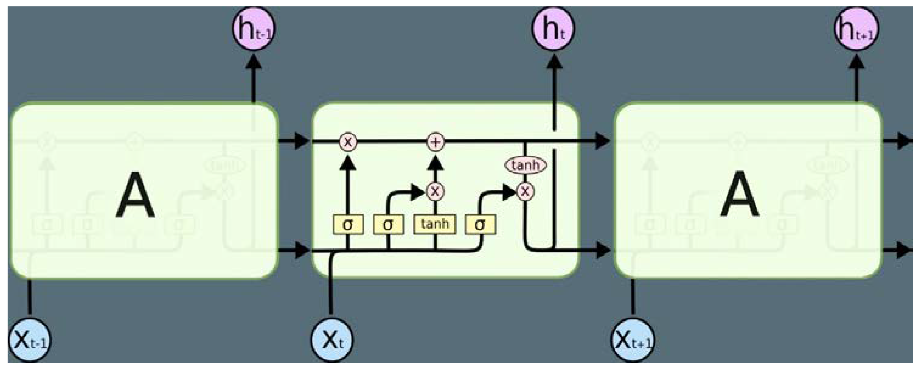Careful regulation of the gate structure is required for the LSTM to add or remove information from nodes to change the information flow state [6,48]. Figure 10 demonstrates the fundamental LSTM.

Figure 9. An LSTM's sequence component consists of four interacting layers [48].

Figure 9. An LSTM's sequence component consists of four interacting layers [48].

An LSTM is typically comprised of the following gates:

Input gate: After the data is imported, the information must first pass through the input gate. Depending on the state of the cell, the switch selects whether or not to store the information. The input gate consists of two steps. First, the sigmoid layer selects which data needs to be updated. Second, the tanh layer generates new data X_t. They can be included in the state of the cell [43,49,50].

Output gate: The output gate determines how much information can be output. First, the sigmoid layer generates an initial output by scaling X_t with tanh to [–1,1]. Finally, the output of the model can be generated by multiplying the sigmoid output pair by pair [43,49].

Forgot gate: The sigmoid in the forget gate is in charge of controlling this. According to a ft value, which ranges between 0 and 1, it determines whether to allow the information collected (X_t-1) to flow. An LSTM layer exists in the LSTM neural network. The surrounding neurons in the same layer are also affected along with the output layer [43,51].

3.3.1. LSTM in Univariate Time Series Forecasting

LSTM (Long Short-Term Memory) is a type of recurrent neural network (RNN) designed explicitly for processing sequential data, such as time series. LSTM has been shown to be very effective in univariate time series forecasting and, in many cases, outperforms traditional statistical methods such as ARIMA and exponential smoothing [43,49,50,51].

The power of LSTM in univariate time series forecasting lies in its ability to capture complex patterns and relationships within the data [50]. Unlike traditional statistical methods, LSTM can capture non-linear dependencies and long-term dependencies within the data. This makes it ideal for modeling time series data that contains trends, seasonality, and other complex patterns [47,48].

LSTM has proven to be a powerful tool for univariate time series forecasting and has been successfully used for various applications, including financial forecasting, energy demand forecasting, and weather forecasting.

3.4. Evaluation Metrics

A widely popular evaluation metric, Mean Square Error (MSE), is used to evaluate models. MSE evaluates the mean squared deviation between the predicted and actual data value and averages it across the entire train or test dataset since MSE can be used in both situations [52]. The value of MSE is always positive since it is always taking the square of error. The following equation define the MSE:

$$\mathrm{M}\mathrm{S}\mathrm{E}=\frac{1}{N}{\sum }_{i=1}^N(y_i-{\widehat{y}}_i{)}^2$$

(6)

Where N represents the population or number of data points, $y_i$ is the actual values, and ${\widehat{y}}_i$ is the predicted values. The MSE is excellent for assuring that our trained model does not contain outlier predictions with significant errors since it gives more weight to these errors thanks to the squaring component of the function. However, in many practical situations, we do not worry about such outliers and instead seek a balanced model that performs satisfactorily on the majority.

4. Result and Discussion

This study's experiment is based on wave speed, direction modeling, and forecasting using a numerical method and artificial intelligence techniques. We used two numerical methods, finite difference, and spectral element methods, to simulate wave speed and direction and compare the result with analytical solutions using Python codes. In the second part, we used LSTM stacking to forecast wave speed and direction in two units of measurement.

4.1. Wave Speed Simulation using Centered Finite Difference Method

The code is a Python script that models a wave propagating along a one-dimensional sea surface using the centered difference method. The wave speed c is set to 1 and the wavelength $\lambda$ is set to 1. The total simulation time T is set to 2, with a space step of $d$x 0.01 and a time step of dt = 0.001

The script first sets up a grid of points on the sea surface with a total of Nx = len(x) points and a total of Nt = len(t) time steps. The wave is characterized by its amplitude A, and its wavelength k and frequency f are calculated from these parameters.

The initial condition of the wave is set to be a sinusoidal wave of amplitude A, and the wave equation is solved numerically for each time step using the centered difference method.

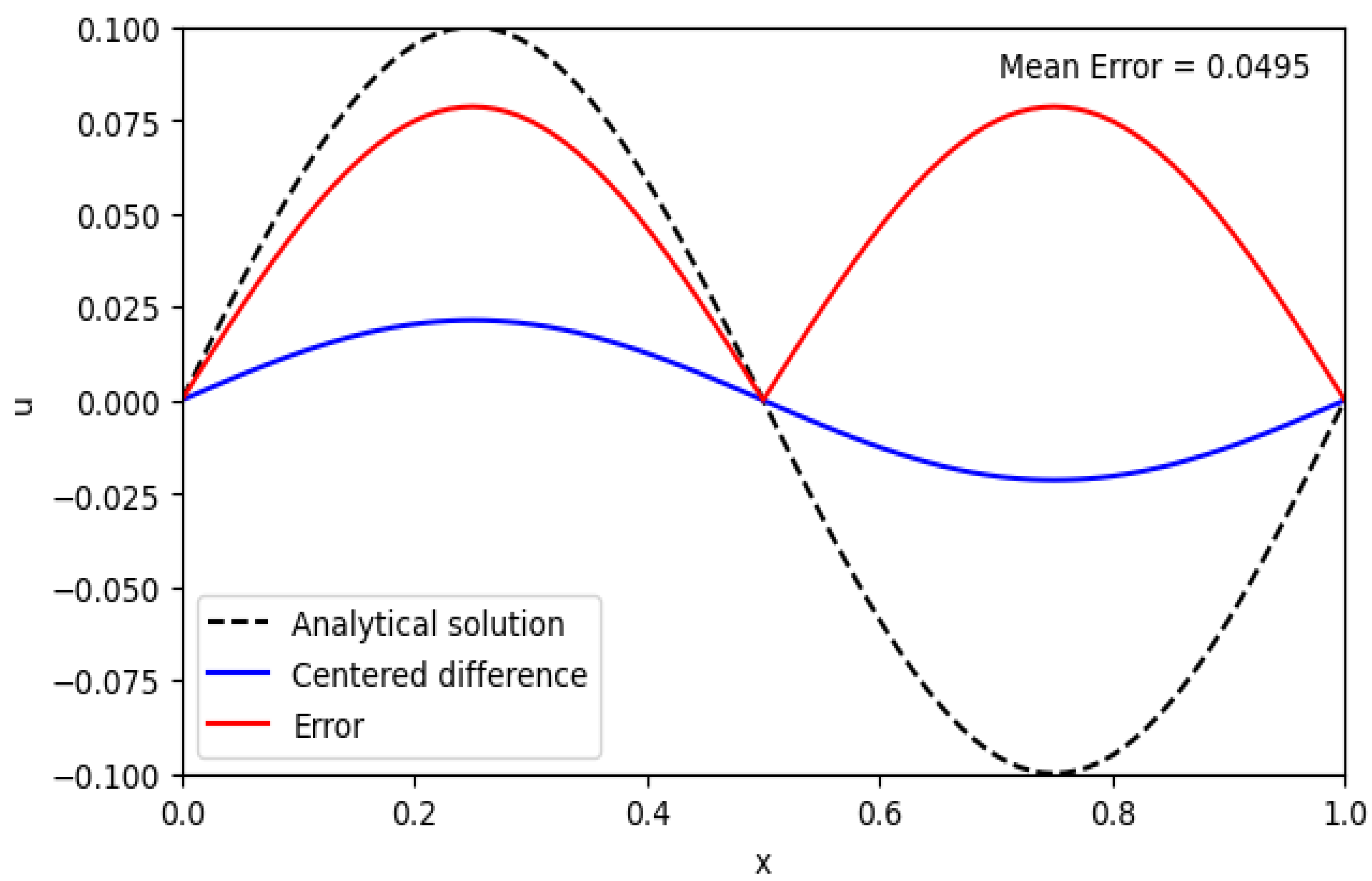
The analytical solution is also calculated for comparison, and the error between the numerical and analytical solutions is plotted at the end of the simulation. The mean error between the numerical and the analytical solution is calculated and displayed as shown in Figure 11.

Figure 10. Wave speed simulation.

Figure 10. Wave speed simulation.

4.2. Wave Direction Simulation using Fast Fourier Transformation

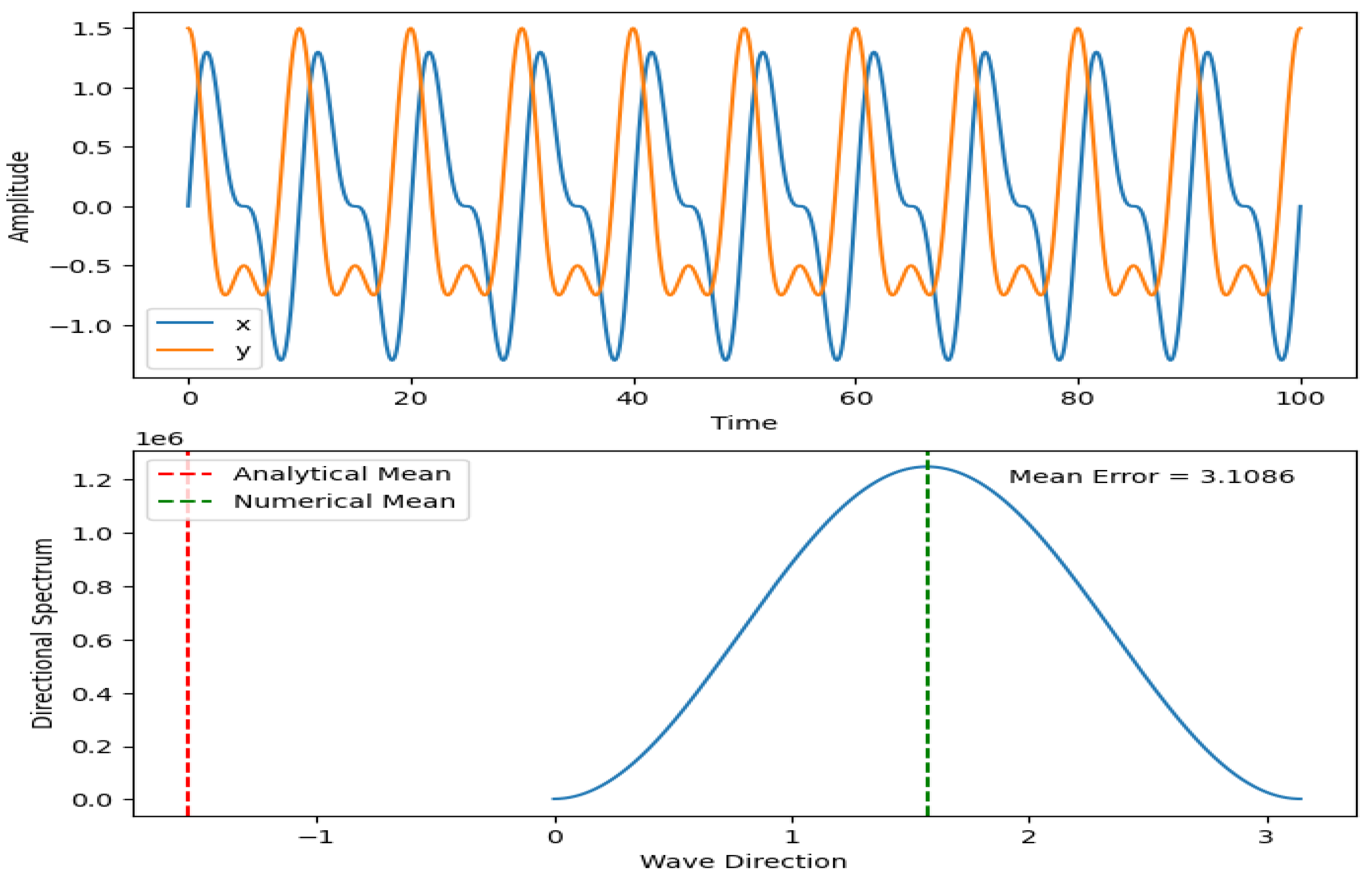
In this simulation, we first generate sample wave data using a combination of two sinusoidal waves. We then calculate the Fourier transform of the wave data using the fftpack.fft() function from the scipy library. We calculate the power spectrum by taking the square of the absolute value of the Fourier coefficients in each dimension.

To calculate the directional wave spectrum, we first define a set of angles (theta) and initialize an array for the directional spectrum. We then loop over each angle and calculate the directional spectrum using the equation 5 above.

We can use analytical and numerical methods to determine the mean wave direction. The analytical method determines the angle of maximum power in the power spectrum. The numerical method determines the angle of the maximum value in the directional spectrum. Then the results are plotted as shown in Figure 12.

Figure 11. Wave direction simulation.

Figure 11. Wave direction simulation.

4.3. Wave Condition Forecasting with LSTM

This study's experiment is based on the wave direction and speed forecast, which consists of 4925 data points. Initially, the model training and validation were performed using a Keras tuner. The epoch versus loss and metric (mean squared error) graph was plotted using Tensorboard for each forecast experiment. The best model was tested with the test dataset, and the mean squared error was measured for each forecast experiment. The results of the experiment will be discussed in detail in this section.

4.3.1. Wave Direction Forecast (Degree)

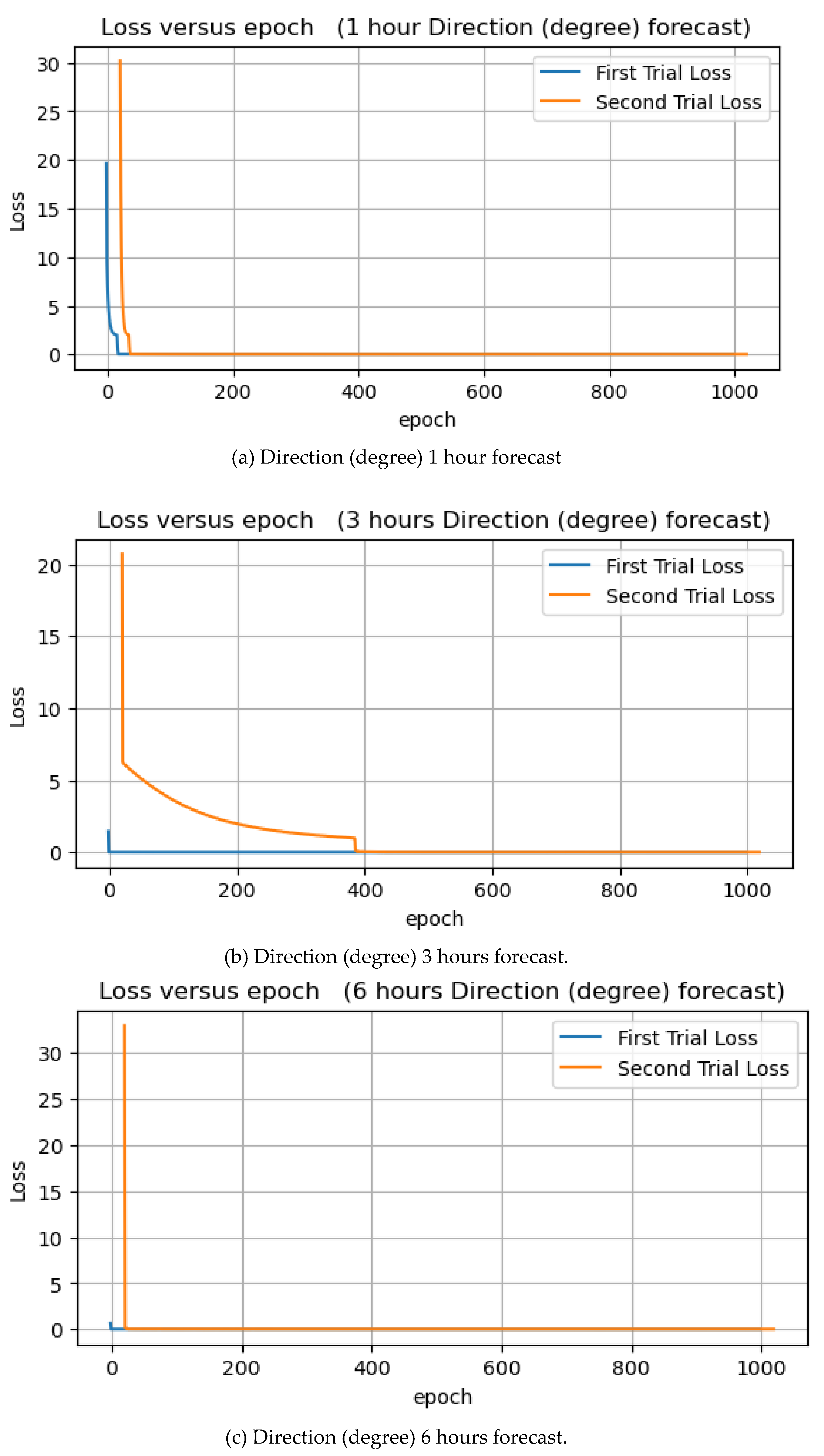
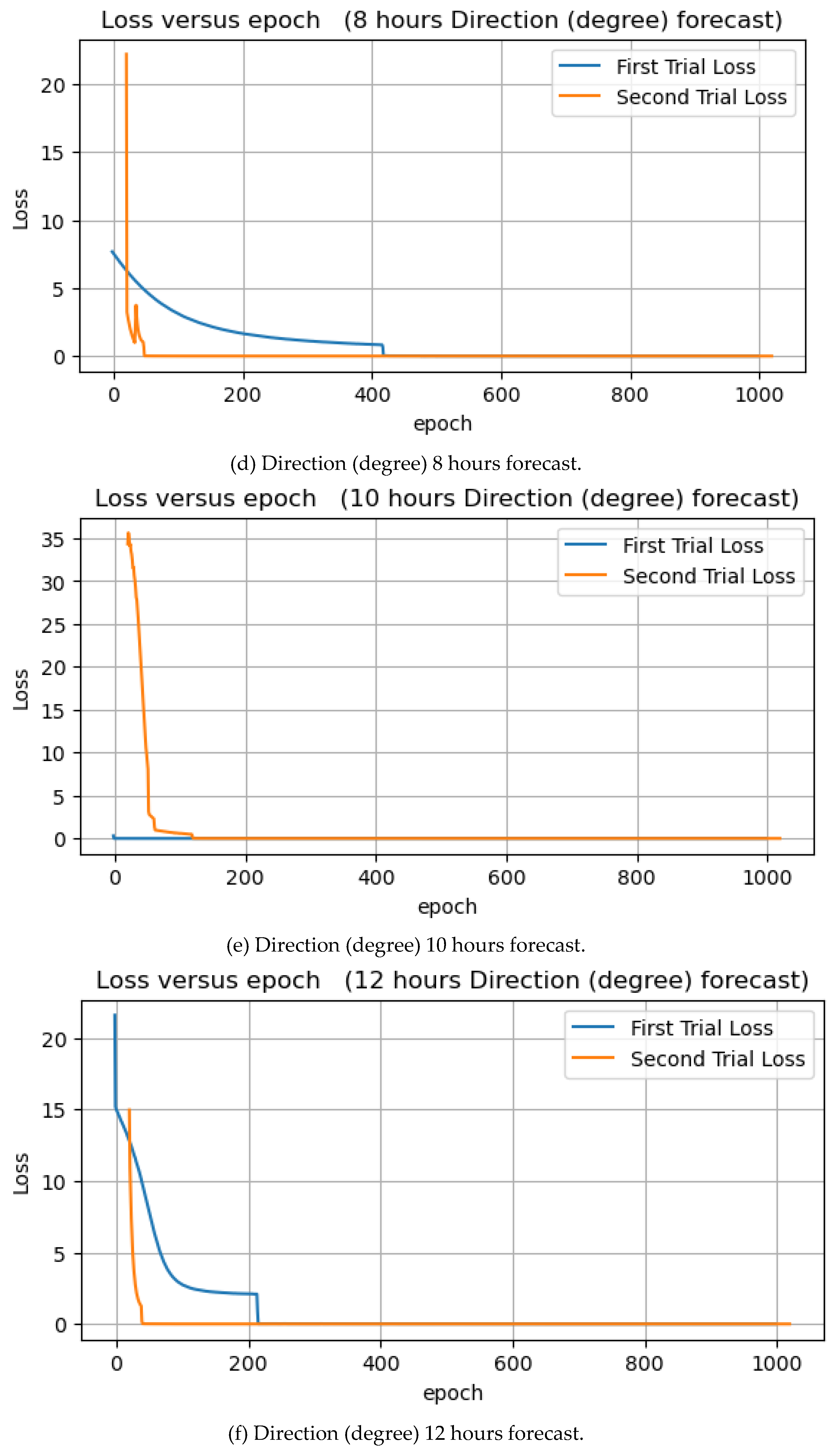
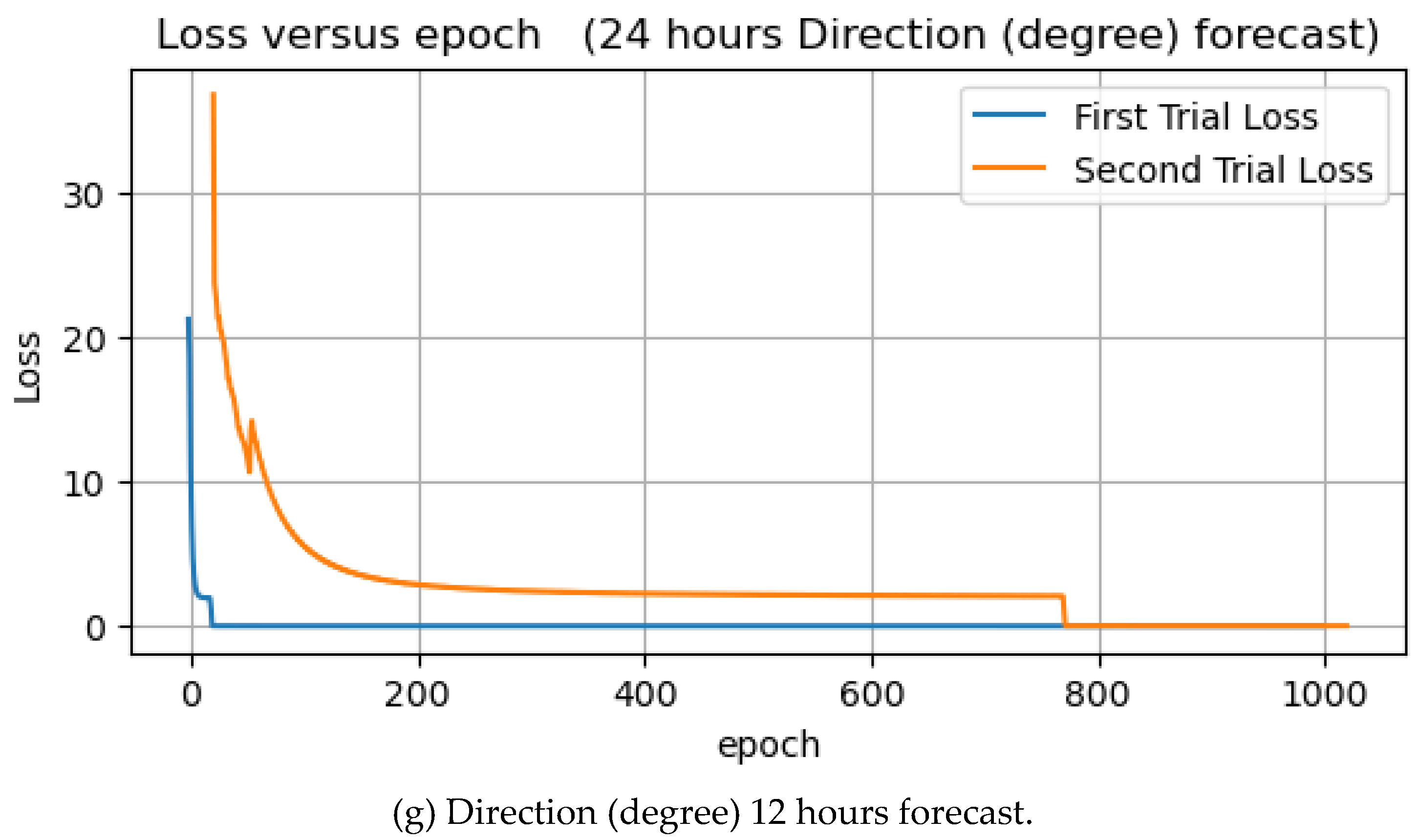
In this experiment, wave direction forecasts were performed using degree and radian units. The main essence of running two wave direction forecasts in two different units of measurement is to identify the unit that can fit our model very well with minor prediction errors. This subsection will discuss and analyze the wave direction forecast in degree units. Figure 12 below illustrate the learning curve of wave direction forecasts.

Figure 12. Direction forecasts of 1, 3, 6, 8, 10, 12, and 24 hours.

Figure 12. Direction forecasts of 1, 3, 6, 8, 10, 12, and 24 hours.

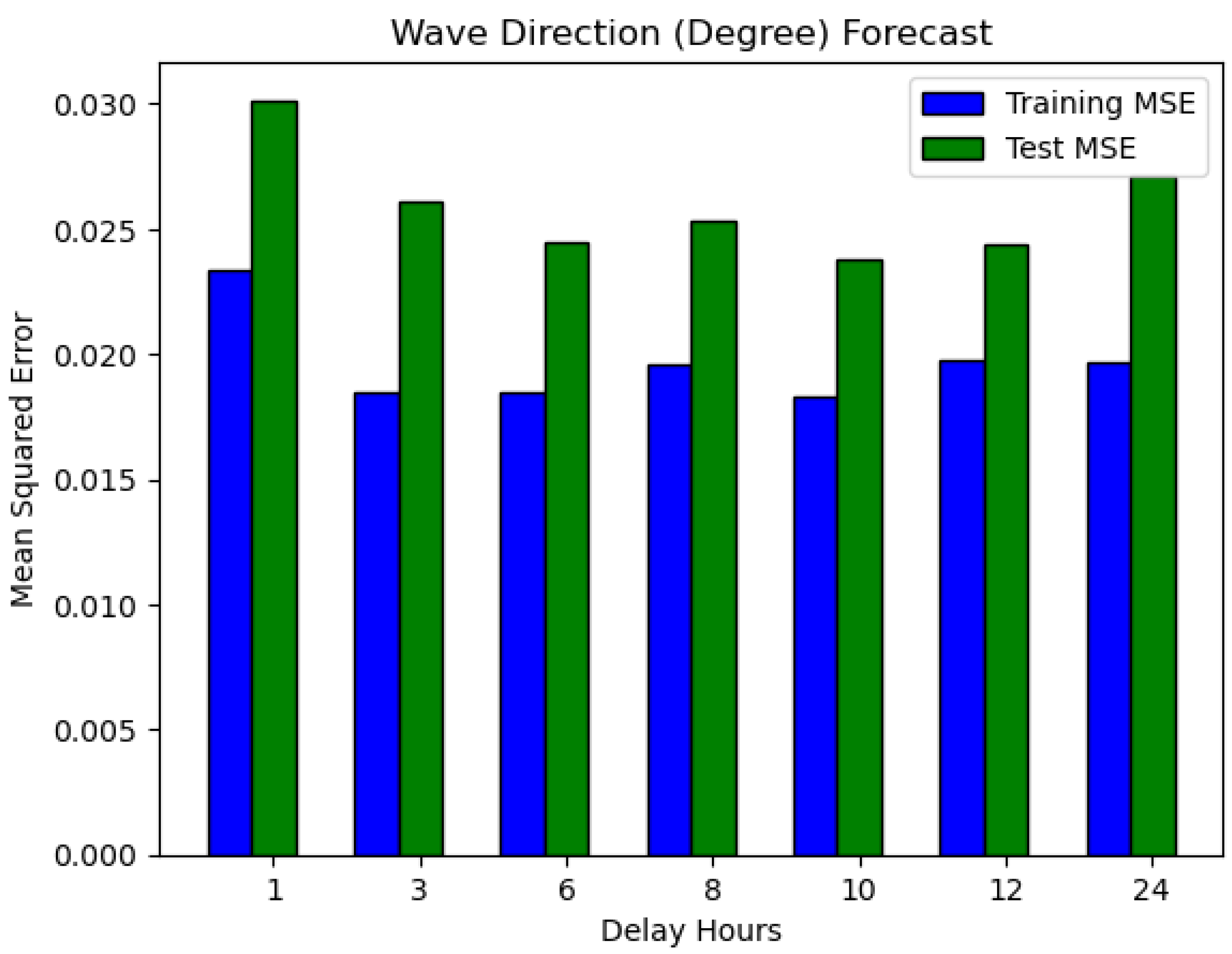
Table 1 contains the experimental results. The forecast of wave direction (degrees) for the next 10 hours has the lowest MSE for training and testing. In contrast, the prediction for the next 1 hour has the highest MSE for training and testing. The predictions for the next 3 and 6 hours also have low training and test errors. Epoch loss decreased to zero at some point in both the first and second trials.

Figure 13 illustrates the training and test MSEs result in form of bar chart, and as expected, the test values are higher than the training values. The model is familiar with the training dataset and knows nothing about the test dataset. That is why the mean squared errors of the test are higher when compared to that of training. The average errors from 7 experiments for training and testing are 0.019 and 0.0259, respectively.

4.3.2. Wave Direction Forecast (Radian)

The second wave direction predictions used radian units instead of the default unit degree. As part of the preprocessing of our data, the wave direction dataset in the dataframe was initially converted to a NumPy array. We then used the function numpy. radians and another dataframe were created and assigned the converted degree to radian values. This subsection analyzes the seven forecasts using the wave direction dataset in the radian unit.

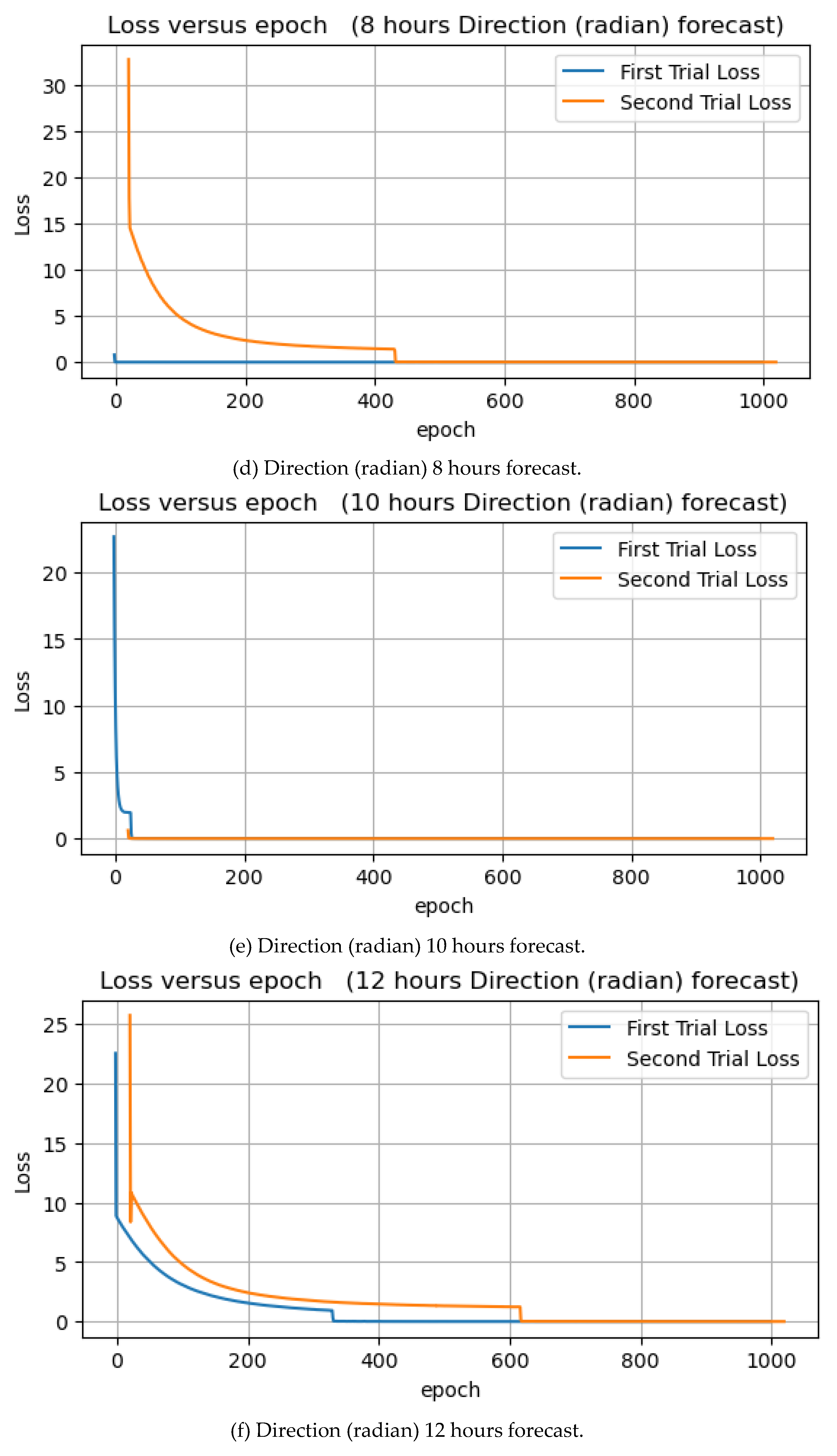
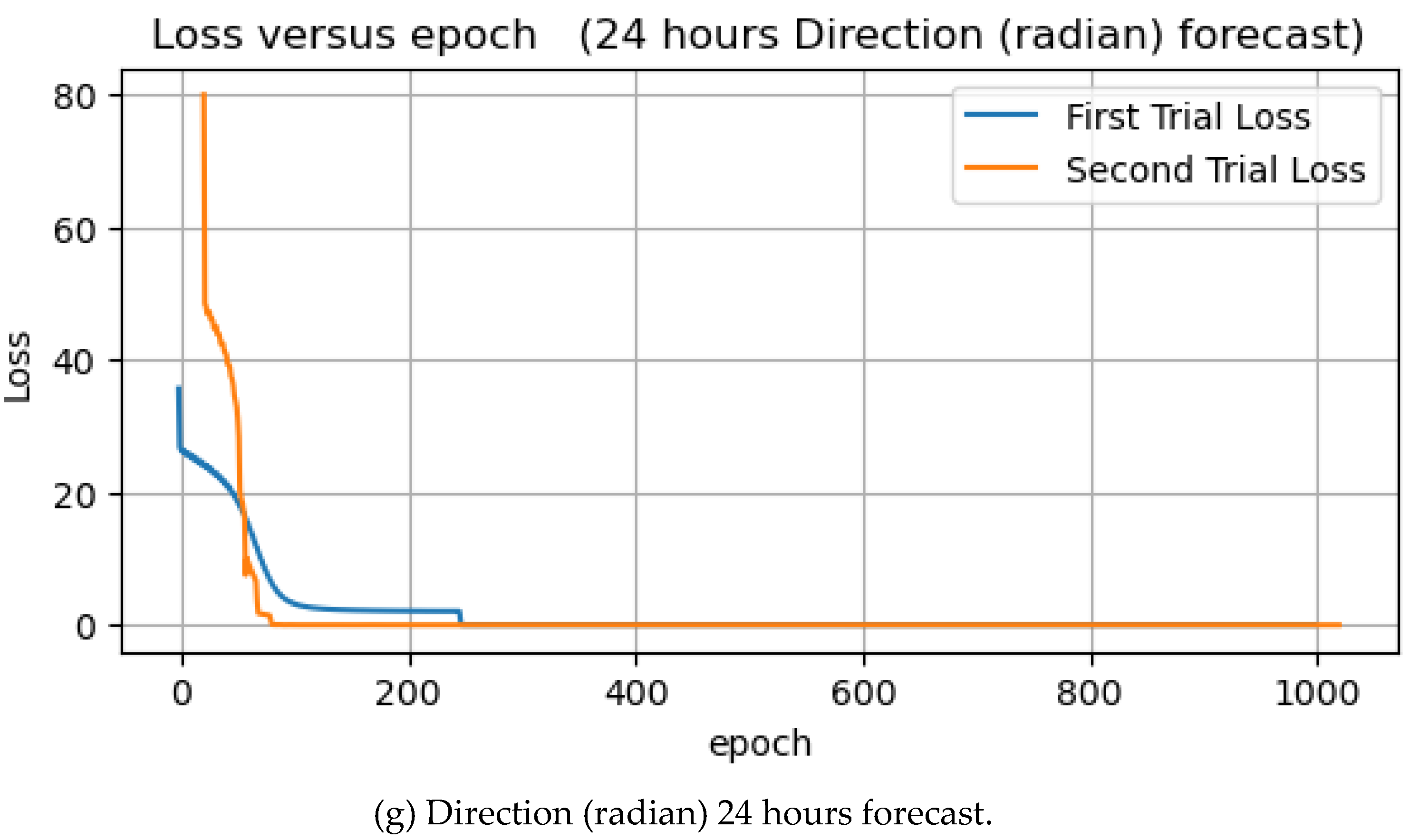
Figure 14. Direction forecasts of 1, 3, 6, 8, 10, 12, and 24 hours in radian units.

Figure 14. Direction forecasts of 1, 3, 6, 8, 10, 12, and 24 hours in radian units.

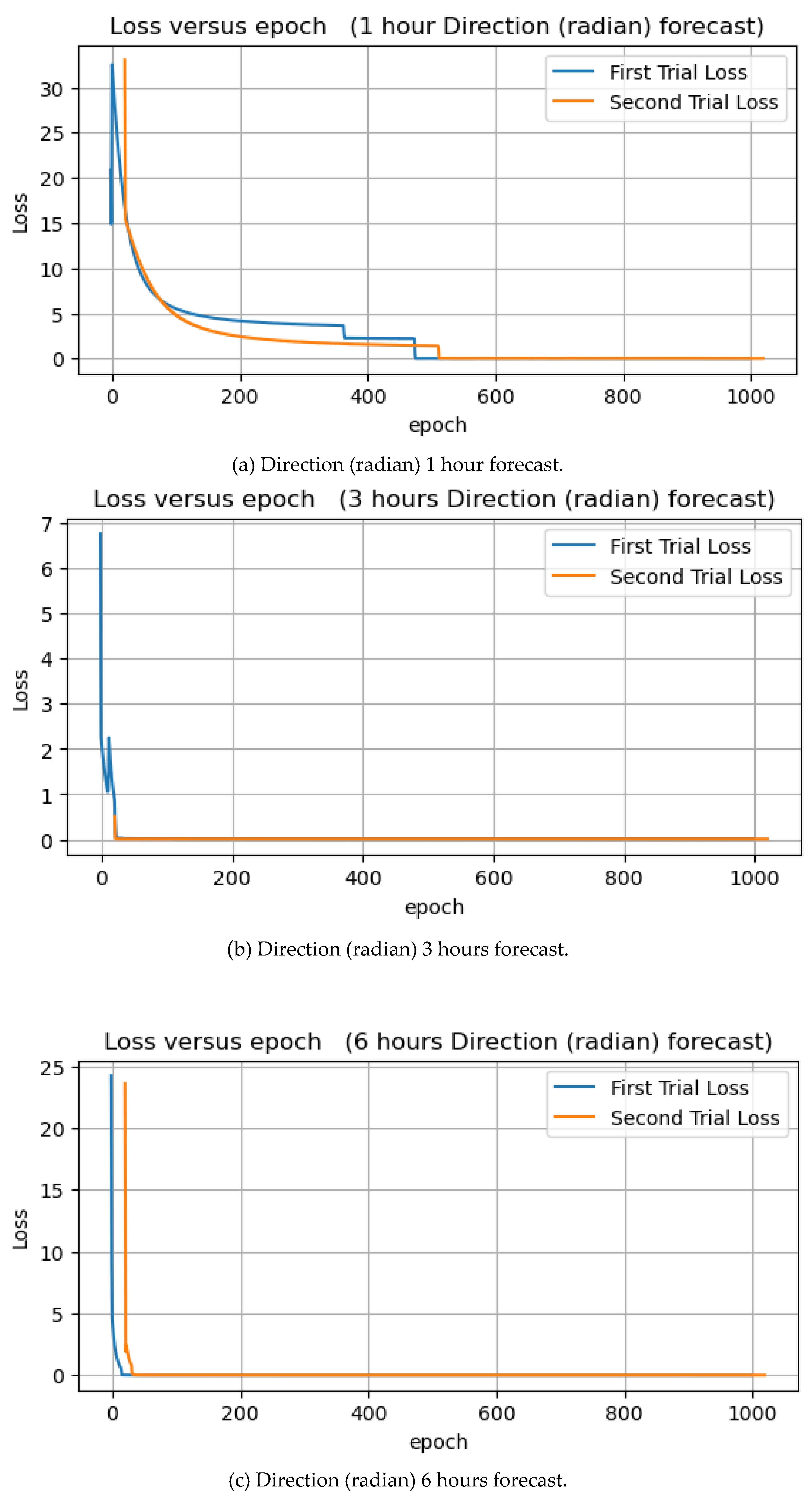
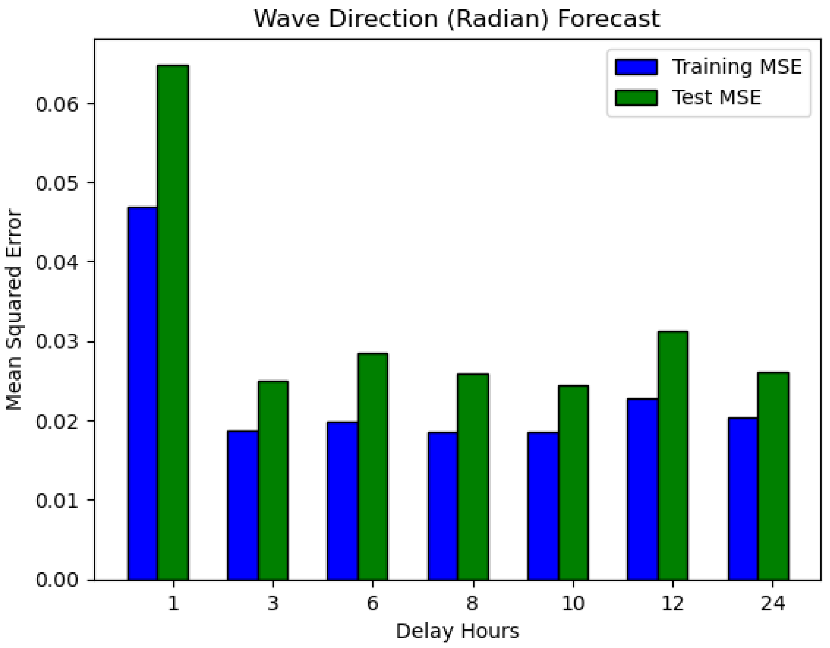
Table 2 shows the experimental results of wave direction forecast in radian units, as in the previous experiments with degree units, with the next 10 hours of prediction showing the lowest MSE in both training and test situations. Moreover, in this experiment the forecasts for the next 10 hours have the lowest training and test errors. In contrast, 1 hour has the highest training and testing error.

Figure 15 illustrates the training and test MSEs; compared to the previous experiment result, the test MSEs are higher than training, which is quite good. The average errors for training and test are 0.0237 and 0.0322, respectively.

The learning curves of epoch versus loss are shown in Figure 15. In all seven experiments, the loss dropped to zero at some points in both the first and second trials.

4.3.3. Comparison of Wave Direction Forecast in Degree and Radian Units

The main objective of using two different direction units is to find the one with the least forecast error. When forecasting wave direction in both units of measure, the epoch loss will eventually be zero. The forecast for the next 10 hours has the lowest training and testing errors in both units. For an 8-hours forecast in a degree unit, the training and test MSE is much higher than for a radiant unit. For the remaining experiments, the errors of forecast in degree units are slightly lower. When comparing forecast in two different units, the training and test errors are very close because the error margins in the corresponding forecast hours are minimal. As can be seen from Table 1 and Table 2, the 24-hour forecasts in radian units are more expensive than the forecasts in degree units.

4.3.4. Wave Speed Forecast

The wave speed was measured in it is default unit (ms^-1 ). This subsection analyzes the seven forecast experiments using the wave speed dataset.

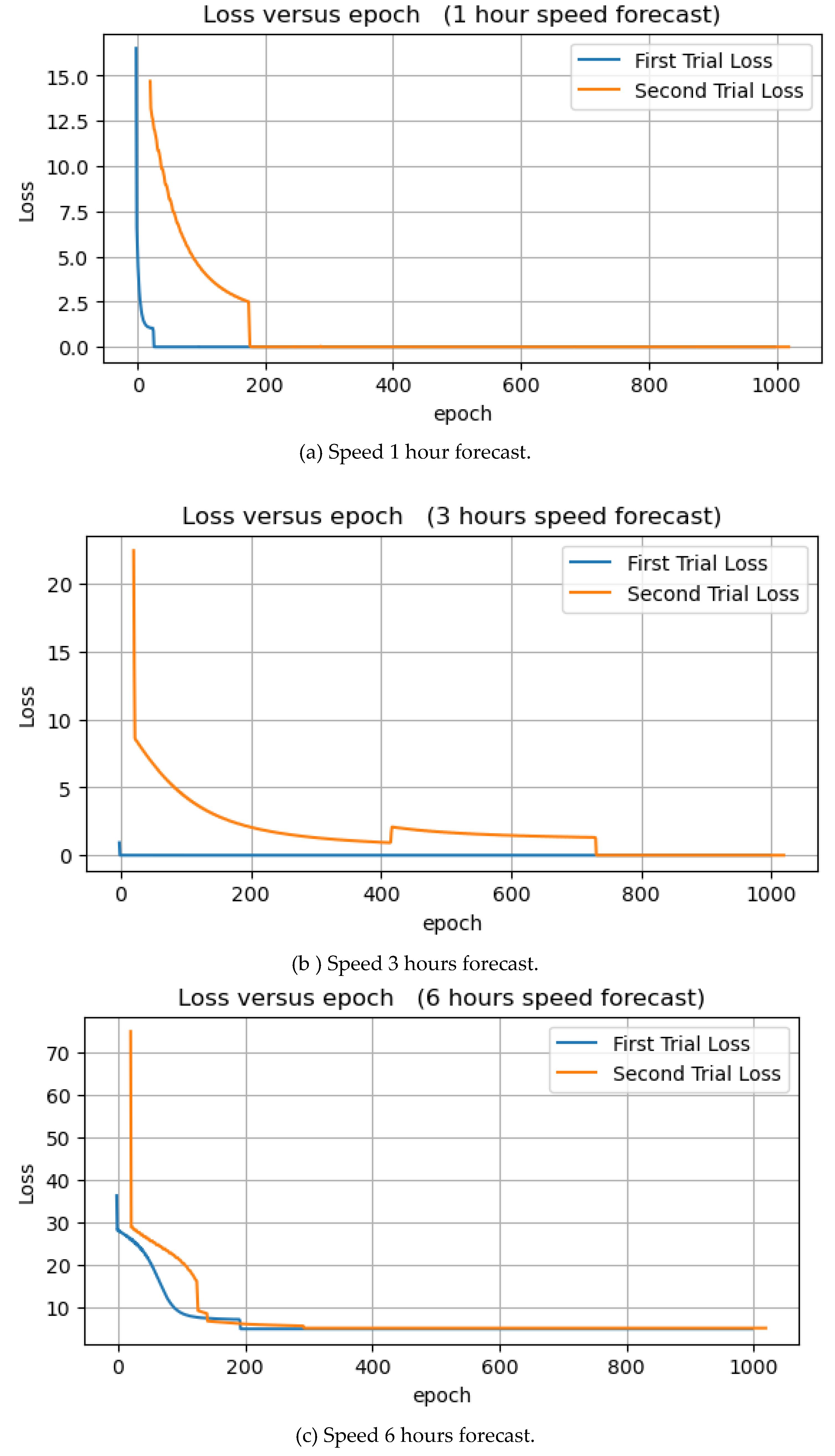
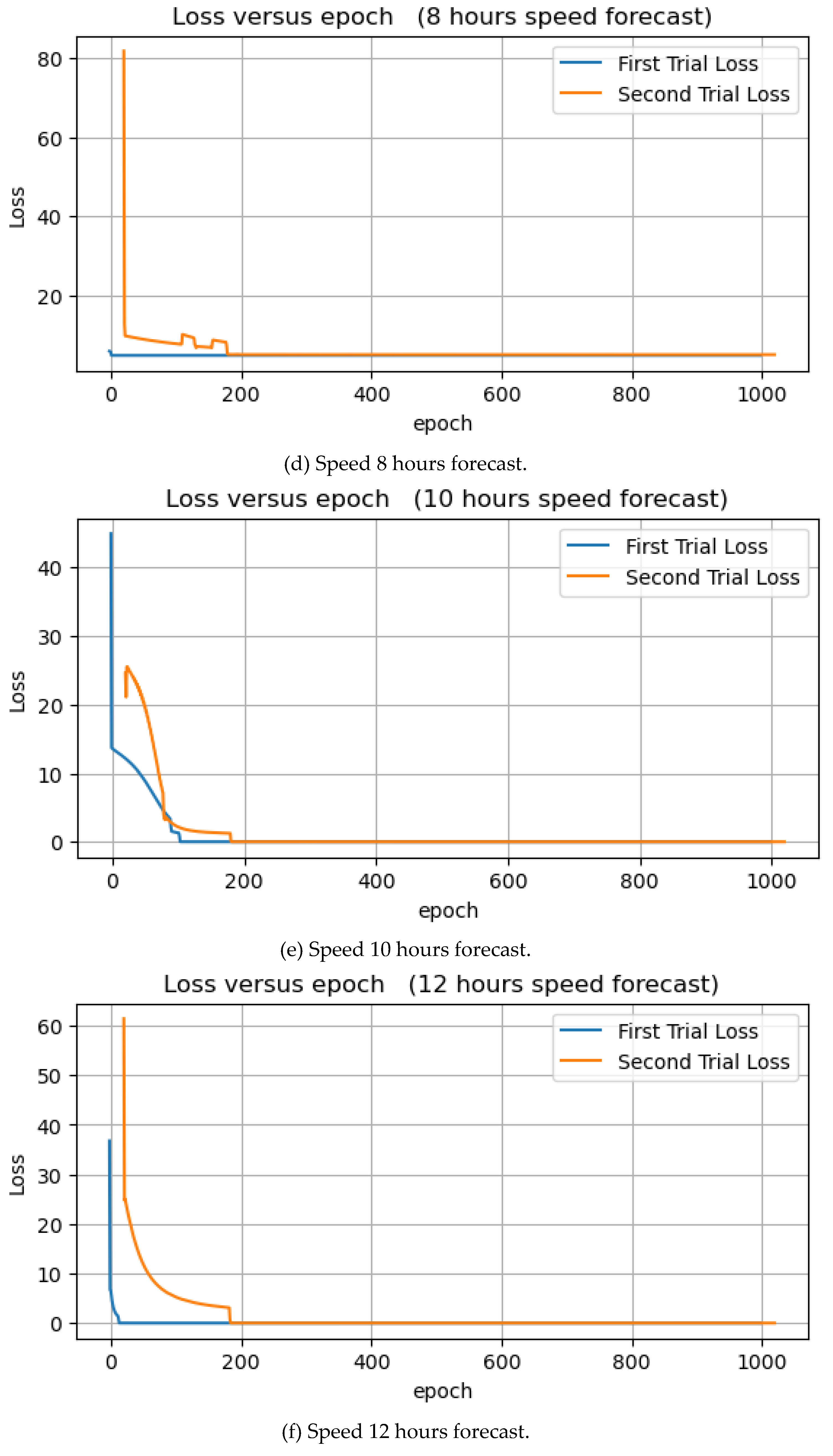
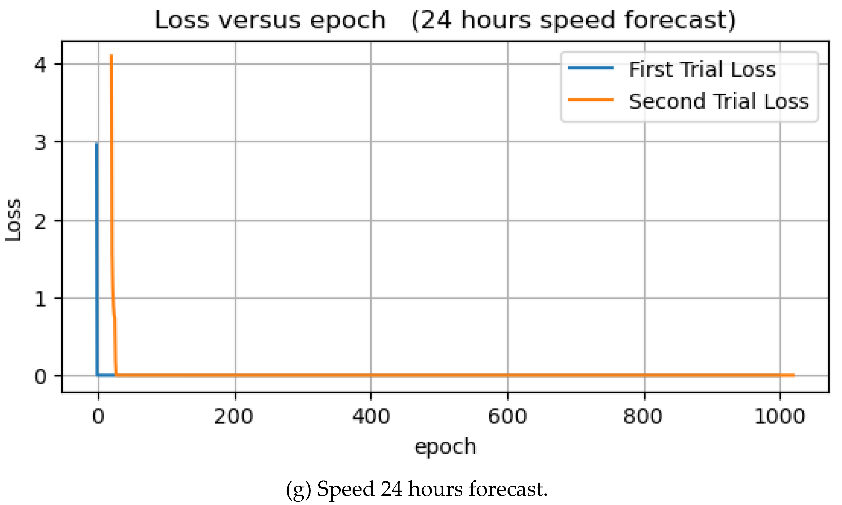
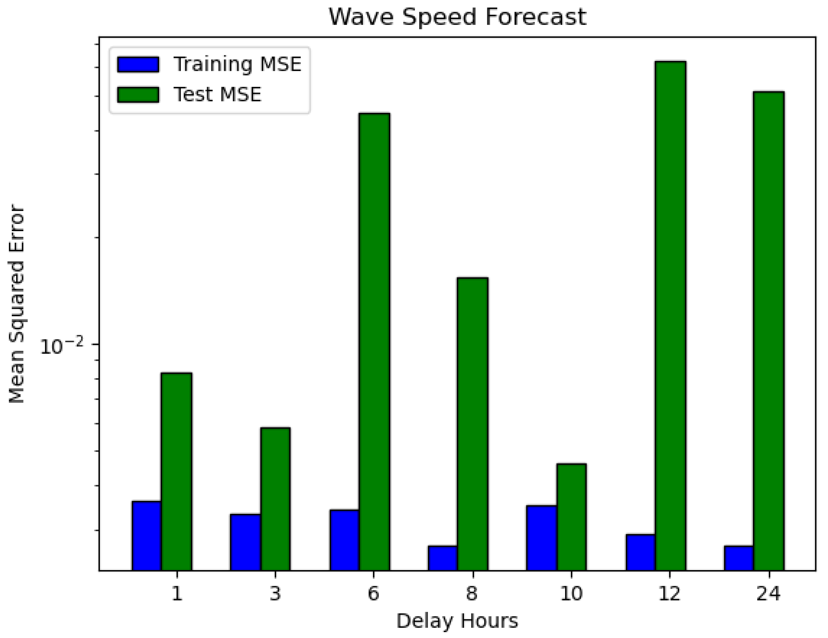
Table 3 shows the experimental results of wave speed forecasts. The forecast of wave speed for 8 and 24 hours has the lowest training MSE of 0.0027, while the forecast for the next 1 hour has the highest training MSE. Conversely, the forecast for 3 and 12 hours has the lowest and highest test MSE, respectively. The learning curves are shown in Figure 16. In each of the seven experiments, the loss dropped to zero at some point.

Figure 17 shows the training and test MSEs. The graph shows that the test MSEs are higher than the training MSEs in all seven-speed forecast experiments, which is similar to the two previous experiments in Figure 3 and Figure 5, which followed the same pattern. The data set was shuffled in each experiment to allow the models to learn perfectly and avoid sampling bias.

However, when we compared the training and test MSEs of forecasting wave speed and direction in two different units of measurement, the former had the least forecast errors when compared with the latter. As for the running cost, the elapsed time for the 24-hour speed forecast is higher than the others, as shown in Table 3.

5. Future Research Direction

The wave equation we used to model ocean wave speed in numerical simulations may need to be revised to capture ocean waves' complex behavior accurately. In the future, we will use higher-order partial differential equations that can solve complex system problems more accurately. The LSTM models proposed in this study were developed using univariate time series techniques, which limit the forecast of wave conditions to only one element at a time. As part of the feasibility and evaluation of marine energy harvesting, we plan to use advanced multivariate time series forecasting and optimization techniques in our future research. In addition, the data we used includes only 4925 data points. In our future study, we plan to collect more data from two or more stations, which could be three or four times the current dataset.

6. Conclusions

This research used two numerical methods to model and simulate the wave speed and direction with sample data. Using a univariate time series approach, we proposed LSTM models to forecast wave speed and direction. We found that the wave speed forecast had less error than direction during the experiment. The forecast of wave direction was performed using two different units of measurement. The forecast in degrees has less error than that in radians. However, the former is slightly less expensive to run when compared to the latter for the 24-hour forecast, despite the differences in prediction in the two units. The error margins and the time difference of the corresponding hours clearly show that each unit's forecast can generate less errors. However, the speed forecast is more expensive to run compared to direction. Using the KerasTuner has simplified the optimization of hyperparameters, which is the secret behind our proposed models with the least MSEs.