Preprint

Article

Numerical Study of Velocity and Mixture Fraction Fields in a Turbulent Non-reacting Propane Jet Flow Issuing into Parallel Co-Flowing Air in Isothermal Condition through OpenFOAM

Altmetrics

Downloads

114

Views

Comments

A peer-reviewed article of this preprint also exists.

Abdolreza Aghajanpour^*,

Seyedalireza Khatibi

Abdolreza Aghajanpour^*,

Seyedalireza Khatibi

This version is not peer-reviewed

Submitted:

12 April 2023

Posted:

13 April 2023

You are already at the latest version

Alerts

Abstract

The present work is a numerical simulation of velocity and mixture fraction fields in a turbulent non-reaction Propane jet flow issuing into parallel co-flowing air, in isothermal condition which has been experimentally described here: http://www.sandia.gov/TNF/DataArch/ProJet.html. The objective is a better understanding of the flow structure and mixing process, a situation in which there is no chemical interaction and heat-transfer. The two-equation Realizable k-ε eddy viscosity turbulence model has been used to simulate the turbulent flow field on a 2D plane (i.e., on a 5-degree sector of the experimental domain), because Realizable k-ε more accurately predicts the spreading rate of both planar and round jets and presents the best proficiency in comparison with all versions of the k-ε models. Afterward, axial and radial profiles of mean velocities, turbulence energy, mean mixture fraction, the mixture fraction half radius (Lf), and the mass flux diagram have been numerically elicited for grid independent mesh (mesh B) and compared with corresponding experimental data to assess the numerical model. To obtain turbulence kinetic energy, k, due to lack of w' in the experimental data, the assumption of w'=v' seems to be valid. Simulations have demonstrated that mean mixture fraction (at radial proﬁles at locations x/D=0, 4, 15, 30 and 50) and its half radius, Lf, which characterizes jet width expanse, are prominently well-captured; Moreover, mean vertical velocity fields (in X-direction: Umean) have revealed less accuracy but still conspicuously well-captured. However, mean vertical velocity fields (in Y-direction: Vmean) have disclosed less resolution; Likewise, turbulence kinetic energy, k, have manifested moderate accuracy (between Umean and Vmean). It should be noticed that although numerical results for absolute pressure, p, have been obtained on aforementioned sections, there were no experimental data to compare with them. Thus, the corresponding numerical data has not been demonstrated in this study.

Keywords:

Subject: Engineering - Mechanical Engineering

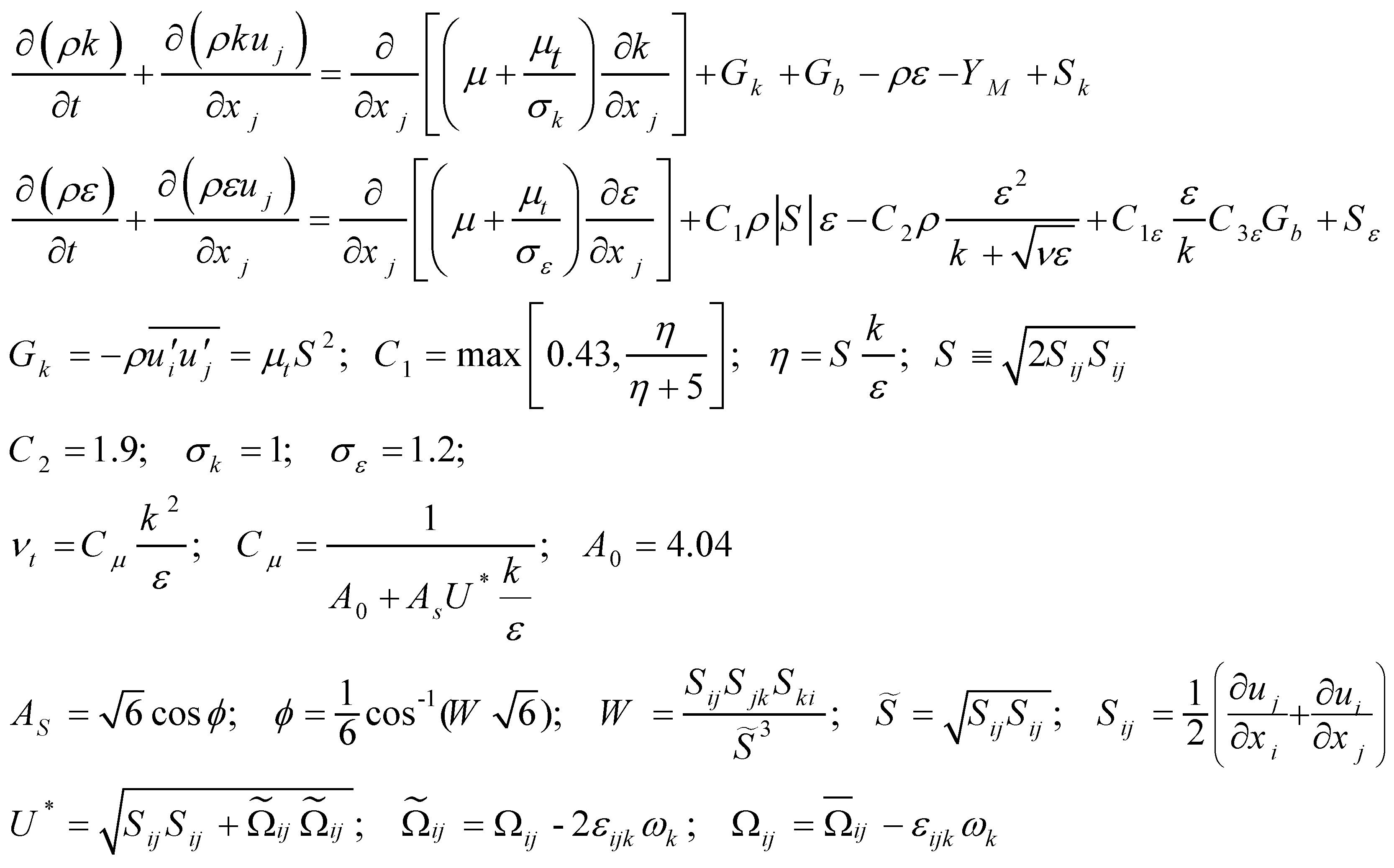
1. Introduction

Turbulent jets emerging from axisymmetric nozzles are pivotal flows classified as free shear layers. The dominating phenomenon is the turbulence due to the velocity gradient and several instabilities between the jet and the surrounding fluid [1]. Besides, re-acting flows are regarded as beneficial branches of turbulent jets, which have vast industrial usages in combustion, military industries engine and so on. Tackling these kinds of jets are generally intricate, because of interactions between turbulent mixing and heat release (due to chemical reactions) [2,3].

Although numerical modeling of turbulent reacting flows is substantially founded on models expanded for non-reacting constant-density flows [3], the use of such models may not be sufficiently authentic [4,5,6]. Having simplified such problem by a turbulent, non-reacting variable-density jet, it is simultaneously conceivable to preserve the intricacy of variable density, and eliminate the elaboration of coupling between turbulent mixing and chemical heat release [3]. In this regard, numerous experimental studies have been carried out on constant-density kinds of turbulent jets [7,8,9,10,11]. Moreover, extensive experiments have been conducted in the scope of strongly variable-density jets through axisymmetric nozzles [12,13,14,15,16,17,18,19,20]. Furthermore, by the advent of progressive laser instruments, it has been feasible to deeply scrutiny the re-acting type of turbulent jets [21,22].

In recent years, by the development of potent computers, the studies have been inclined toward the numerical simulations, due to be cheaper, faster and easier. In this scope, utilization of open source codes has been rapidly more popular, especially the OpenFOAM which has been written in C++ language and allows users to upgrade and develop the system further [1,23].

It should be noticed that the behavior of variable-density turbulent jets is intensively sensitive to the inlet conditions, particularly the injection ratio [24], the direction of the co-flowing and the geometry of the nozzle [2].

In this work, a numerical study has been carried out on a turbulent axisymmetric jet using Realizable k-ε eddy viscosity turbulence model through manipulating and regulating ReactingFoam solver in OpenFOAM 5x, with the aim of investigation of the capability of this procedure in simulating the experimental data which have been presented here: http://www.sandia.gov/TNF/DataArch/ProJet.html. It should be emphasized that ReactingFoam is one of the standard solvers in OpenFOAM which has been particularly extended to resolve the mixing problems of compressible flows involving combustion and reactions.

To simulate this problem, initially, sandiaD_LTS tutorial (in combustion>reactingFoam>RAS) has been regarded as the basement and then has been manipulated through deactivating combustion and reaction from corresponding files due to lack of these phenomena in the experiment.

2. Numerical basement

2.1. Mixture fraction theory

In contrast with premixed systems, in non-premixed combustion, fuel and oxidizer enter the reaction zone in distinct streams [25]. Under certain assumptions, the thermochemistry can be reduced to a single parameter: the mixture fraction, f, the mass fraction that originated from the fuel stream, which is a conserved scalar quantity, and therefore its governing transport equation does not have a source term. Consequently, combustion is simplified to a mixing problem. After mixing, the chemistry can be modeled through Equilibrium model, Steady Diffusion Flamelet or Unsteady Diffusion Flamelet, for being in chemical equilibrium, near that or being meaningfully far from that, respectively [25].

Although the assumption of equal diffusivities of species is problematic for laminar flows, it is generally acceptable for turbulent flows where turbulent convection overwhelms molecular diffusion. Consequently, the species equations can be reduced to a single transport equation for the mixture fraction, f. Non-premixed modeling involves the solution of this equation. Afterward, species concentration can be elicited from the predicted mixture fraction field. Moreover, under a particular set of simplifying assumptions, the instantaneous thermochemical state of the fluid is related to mixture fraction, [25].

The power of the mixture fraction modeling approach is that the chemistry is reduced to one or two conserved mixture fractions. Under the assumption of chemical equilibrium, all thermochemical scalars (species fractions, density, and temperature) are uniquely related to the mixture fraction(s) [25].

2.2. The transport equation for the mixture fraction

The Favre mean (density-averaged) mixture fraction equation is [25]:

\frac{\partial (ρ \bar{f})}{\partial t} + \nabla . (ρ \vec{v} \bar{f}) = \nabla . (ρ \vec{v} \bar{f}) + \frac{\partial}{\partial x_{j}} (\frac{μ_{l} + μ_{t}}{σ_{t}} \nabla \bar{f})

3. Description of computational domain and assumptions

By comparing the inner and outer dimensions of the tube with the aspects of the horizontal cross section of the experimental domain, and regarding the immense differentiation between the bulk velocity of Propane and co-flowing air, the assumption of an axisymmetric problem is not far from the reality. By this assumption, it is conceivable to massively alleviate the needed computational resources. Thus, the computational domain has been confined to a single 2D plane, i.e., a 5-degree sector of the biggest cylinder which can be embedded into the real domain.

There are two strategies for preparing the computational geometry. At first one, a single sector can be defined by neglecting the length of the nozzle. Thus, the flow within the nozzle will not be simulated. In this condition, the inlets boundaries of the Propane and the co-flowing air will be placed at the level of the nozzle exhaust.

In the other approach (as this study), a nozzle (for example, with 10 cm length) can be placed at the upstream to better establish of fully developed flow within the nozzle (before the injection into the principal computational domain), and to better form the boundary layer between the co-flowing air and the outer edge of the nozzle, a phenomenon which has been observed in the experiment. It is evident that the first approach is cheaper and faster because of reduced cell numbers, and presumably less accurate due to attenuate the simulation of the real boundary conditions around the nozzle's body.

Contrary to the Standard k-ε model, in the Realizable k-ε model, C_µ, (the coefficient which is imposed in the equation of turbulent viscosity, ν_t, is not a constant, but a function. It is worthy to notice that although the transport equation of turbulence kinetic energy, k, is the same as that in the Standard and the RNG k-ε models, except for the model constants, the transport equation of its Dissipation Rate , ε, has been modified by extracting the aforementioned equation from the exact equation of the transport of the mean-square vorticity fluctuations. Hence, the Realizable k-ε more accurately predicts the spreading rate of both planar and round jets and presents the best proficiency in comparison with all versions of the k-ε models [26].

By regarding the plotted figures of experimental data and with the aim of more minifying the domain, the length of the computational field has been confined to 100 cm (x/D=190), because no cognizable variations have been observed after x/D>80, in experimental data.

The volume fraction of N2 and O2 in the co-flowing air has been assumed as 0.7632 and 0.2368, respectively. Furthermore, the flow assumed to be compressible and isothermal (294 K), and the injecting fluids are considered to be ideal gasses.

To define the computational domain as a sector and its boundaries, the blockMeshDict, the changeDictionaryDict and the extrudeMeshDict files in the system folder have been utilized. Moreover, inletfuel (inlet boundary of Propane at upstream on the inner diameter of the nozzle), inletair (inlet boundary of co-flowing air at upstream, from outer ridge of the nozzle to the lateral border, leftside), outlet (the outlet boundary at downstream), axis (the axis of symmetry which the sector rotates 5 degrees around that), leftside (the lateral edge of domain), burnerwall (part of upstream boundaries which represents the body of the nozzle), front and back (to simulate a 2D problem) have been defined and adjusted as the boundaries through the blockMeshDict file and the corresponding files of each variable in the 0 folder.

Figure 1 shows a simplified scheme of the computational domain:

Eventually, in order to reduce the computational expenditures, and moreover, to obtain a proper aspect ratio, the grids have manipulated through predefined lengthGrading for both X and Y directions of each block, in blockMeshDict file.

To obtain turbulence kinetic energy, k, we have:

\begin{array}{l} U_{R M S} = \sqrt{\bar{{u^{'}}^{2}}}, V_{R M S} = \sqrt{\bar{{v^{'}}^{2}}}, W_{R M S} = \sqrt{\bar{{w^{'}}^{2}}} \\ \Rightarrow U_{R M S}^{2} = \bar{{u^{'}}^{2}}, V_{R M S}^{2} = \bar{{v^{'}}^{2}}, W_{R M S}^{2} = \bar{{w^{'}}^{2}} \\ k = \frac{1}{2} (\bar{{u^{'}}^{2}} + \bar{{v^{'}}^{2}} + \bar{{w^{'}}^{2}}) = \frac{1}{2} (U_{R M S}^{2} + V_{R M S}^{2} + W_{R M S}^{2}) \end{array}

But, due to the 2D assumption which can be observed in experimental data, it is can be reduced to:

k = \frac{1}{2} (U_{R M S}^{2} + V_{R M S}^{2} + W_{R M S}^{2}) = \frac{1}{2} (U_{R M S}^{2} + 2 V_{R M S}^{2})

Having plotted some non-dimensional parameters, assessment of axial and radial profiles of mean velocities, turbulence energy, mean mixture fraction, and the mixture fraction half radius, and subsequently, the comparison have been fulfilled between corresponding numerical and experimental data.

Table 1 comprises a concise list of computational domain's dimensions and some inlet data:

4. Initial and boundary conditions of variables

Regarding the provided meshes, it is evident that the last computational node on the leftside will be placed out of the boundary layer. In other words, Yplus can't be confined between 30 and 100, which is essential for the correctness of assumption of utilizing the wall functions. Consequently, it is not allowed to use any wall functions. On the other side, due to numerical costs' considerations, at least, it is not logical to refine the mesh toward the outer walls, i.e., leftside.

Thus, in the first approach, by assuming the boundary condition as fixedValue(=9.2) for the velocity, U, and zeroGradient for other variables, it is tried to simulate slip condition on the leftside boundary, which is not far from the reality. Besides, it is assumed that the meshes are refine enough on the inner and outer sides of the nozzle's body, i.e., burnerwall. Afterwards, wall function has been imposed for alphat ,epsilon ,k and nut, and noSlip condition for U.

Moreover, to interrogate the authenticity of such assumptions on nozzle's body, i.e., burnerwall, in some other test cases (the second approach), the mentioned boundary has been partitioned to its three sides: burnerwall_jet, burnerwall_air and burnerwall_upper, and each one of them have been assigned its own boundary conditions for each of the variables. Although the corresponding numerical results have not been presented in this study, but it could not be perceived any significant differentiations, which may approve the assumptions of first's approach.

Table 2 and Table 3 comprise a brief list of initial and boundary conditions for diverse variables, for the first approach. But, similar information for the second one has not been presented here for abbreviation:

It should be noticed that all of the variables have been introduced as empty to the axis boundary because it is an edge of the domain, not a surface. Additionally, wedge has been assigned to front and back boundaries, simultaneously, because they have been defined as two repetitive sides of the sector.

In this study, at inletfuel, by assuming

{Re}_{D, f u e l} = 68000

C_{μ} = 0.09

and

D_{h, f u e l} = 5.26 m m

for fully turbulent Propane jet, the turbulent intensity (turbulence level) ,

I

, the boundary condition for turbulence kinetic energy, k, and the boundary condition for its dissipation rate, ε, have been successively calculated as [25]:

I_{i n l e t, f u e l} = 0.16 {Re}_{D, f u e l}^{\frac{- 1}{8}} ≃ 0.0398

k_{i n l e t, f u e l} = \frac{3}{2} {(U . I)}^{2} ≃ 6.679

l_{i n l e t, f u e l} = 0.07 D_{h, f u e l} = 0.000368 m

ε_{i n l e t} = C_{μ}^{\frac{3}{4}} k_{i n l e t, f u e l}^{\frac{3}{2}} l_{i n l e t, f u e l}^{- 1} ≃ 5630

Moreover, at inletair, by assuming

I_{inlet, a i r} = 0.004

C_{μ} = 0.09

and

D_{h, a i r} = 30 c m

for turbulent co-flowing air, we have these boundary conditions:

k_{i n l e t, a i r} = \frac{3}{2} {(U . I)}^{2} ≃ 0.002

l_{i n l e t, a i r} = 0.07 D_{h, a i r} = 0.021 m

ε_{i n l e t, a i r} = C_{μ}^{\frac{3}{4}} k_{i n l e t, a i r}^{\frac{3}{2}} l_{i n l e t, a i r}^{- 1} ≃ 0.0006998

Although it is clear that the steady-state results depend on the boundary conditions, not the initial values, it is tried to assign the logical initial values for various variables.

5. Other governing equations [25]

5.1. Mass Conservation Equation

\frac{\partial ρ}{\partial t} + \nabla . (ρ \vec{U}) = 0

5.2. Energy Conservation Equation

\frac{\partial}{\partial t} (ρ E) + \nabla . (\vec{U} (ρ E + p)) = - \nabla \sum_{j} h_{j} J_{j} + S_{h}

5.3. Momentum Conservation Equations

\frac{\partial (ρ \vec{U})}{\partial t} + \nabla . (ρ \vec{U} \vec{U}) = - \nabla p + ρ \vec{g} + \vec{F}

(1)

5.4. Transport equations for turbulence kinetic energy, k, and its dissipation rate, ε, [26,27,28]

6. Numerical discretizing schemes

Table 4 comprises a detailed list of assigned discretizing schemes for diverse terms:

7. Solution procedures

Due to lack of combustion and reaction in the experiment, the files of the constant folder have been modified to eliminate these phenome in the numerical test cases. The set of governing equations have been resolved through PIMPLE algorithm by setting nOuterCorrectors, nCorrectors, nNonOrthogonalCorrections, and relaxationFactors to 1, 2, 0 and 1, respectively.

In an entirely transient simulation of such problem, at first, slower fluid's requisite time of passing the entire of the domain should be obtained. Typically, 15 to 20 times of that is sufficient as the total required time of simulating. Moreover, the corresponding time step can be elicited by limiting the Courant number to 3 or 4 (it depends on the nature of the problem and trial and error). But in this study, because just the steady-state needs to be regarded, to accelerate a solution to such condition, local-time stepping method has been used (i.e., pseudo-transient simulation), by adjusting the discretizing scheme of temporal terms to localEuler. Therefore, both endTime and deltaT which are introduced to controlDict file have no physical meaning and represent the number of iterations.

Moreover, in the fvSolution file, tolerance (the convergence level) has been adjusted to 10e-08 and 10e-06 for Yi (species) and all of the other variables, respectively.

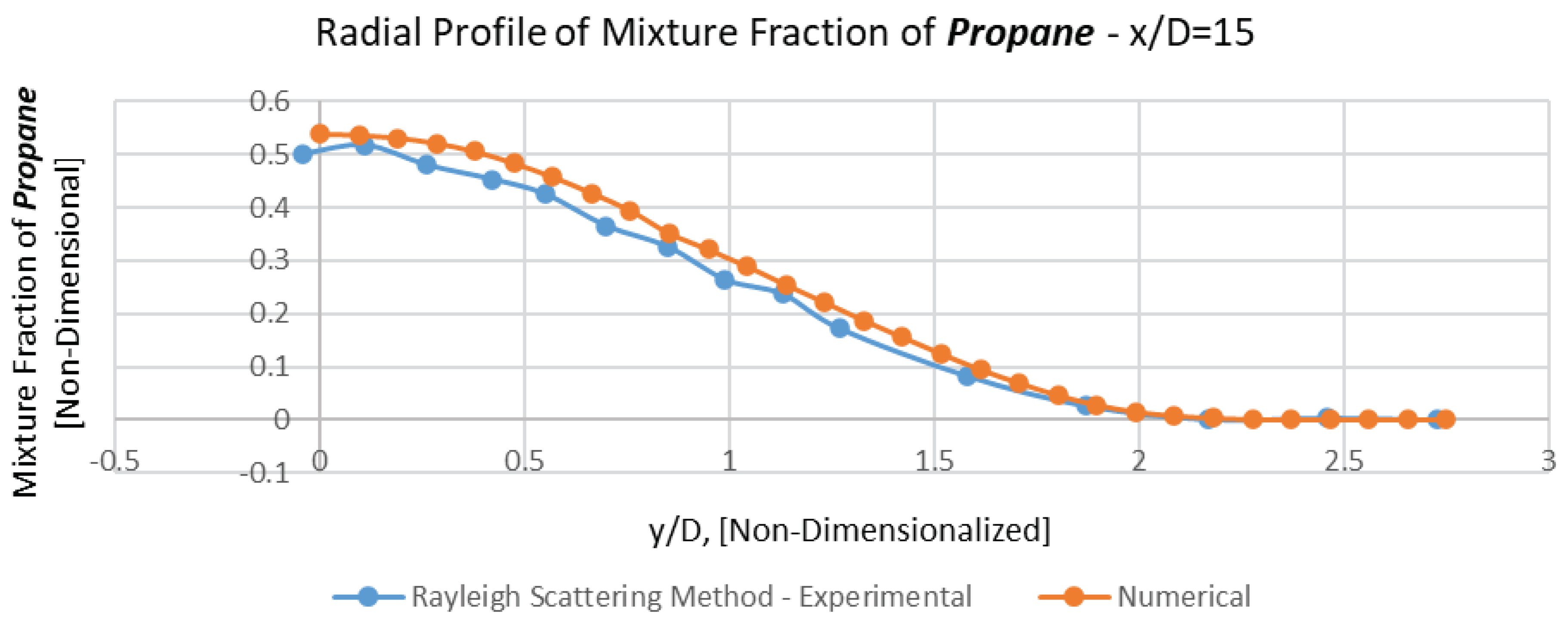
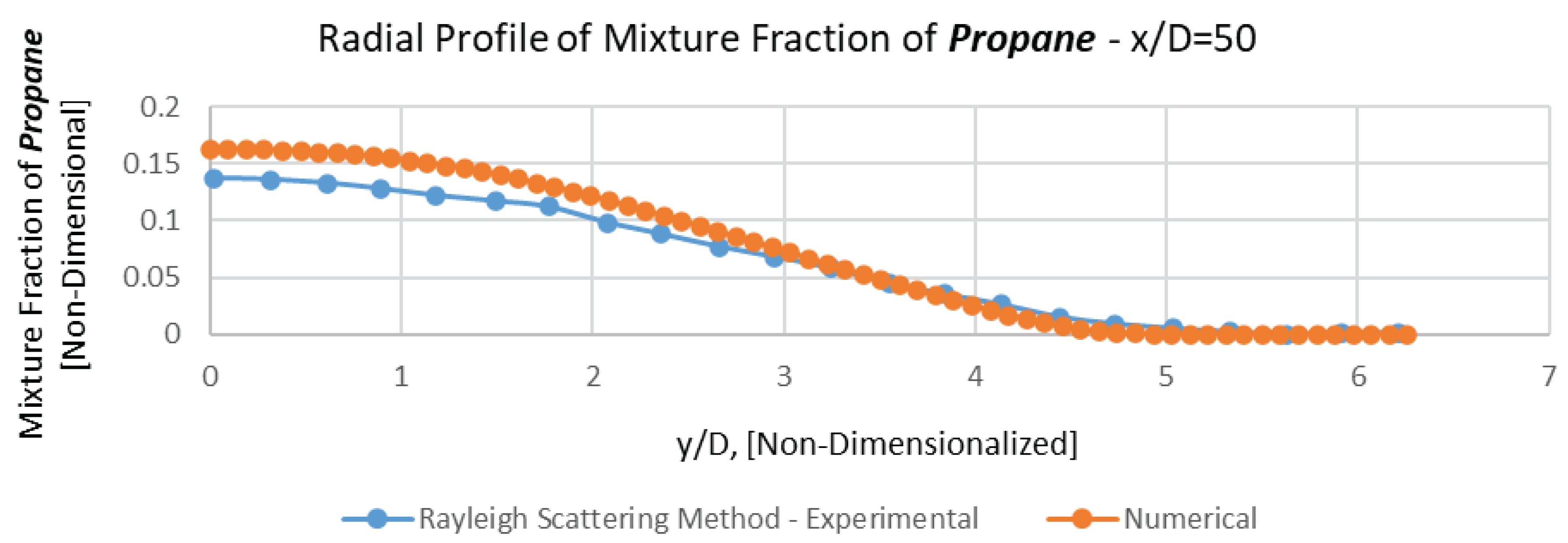
In the sampleDict file of the system folder, required data have been introduced on x/D=0, 4, 15, 30 and 50, and also adjacent to axis boundary (y/D=0), each on 101 points. Subsequently, although these data have been plotted in the createGraphs folder of each test case by the gnuplot, the corresponding data have been obtained from the results which have been recorded by OpenFOAM, for the last iteration, in postProcessing>sample>30000 folder of each test cases. Eventually, the mentioned data have been transferred to Excel and plotted alongside the experimental data to compare with each other, as have been shown in Figures 6 to 28 at the end of this study.

Initially, as it has been demonstrated in Table 5, four meshes with different cells and aspect ratios have been created:

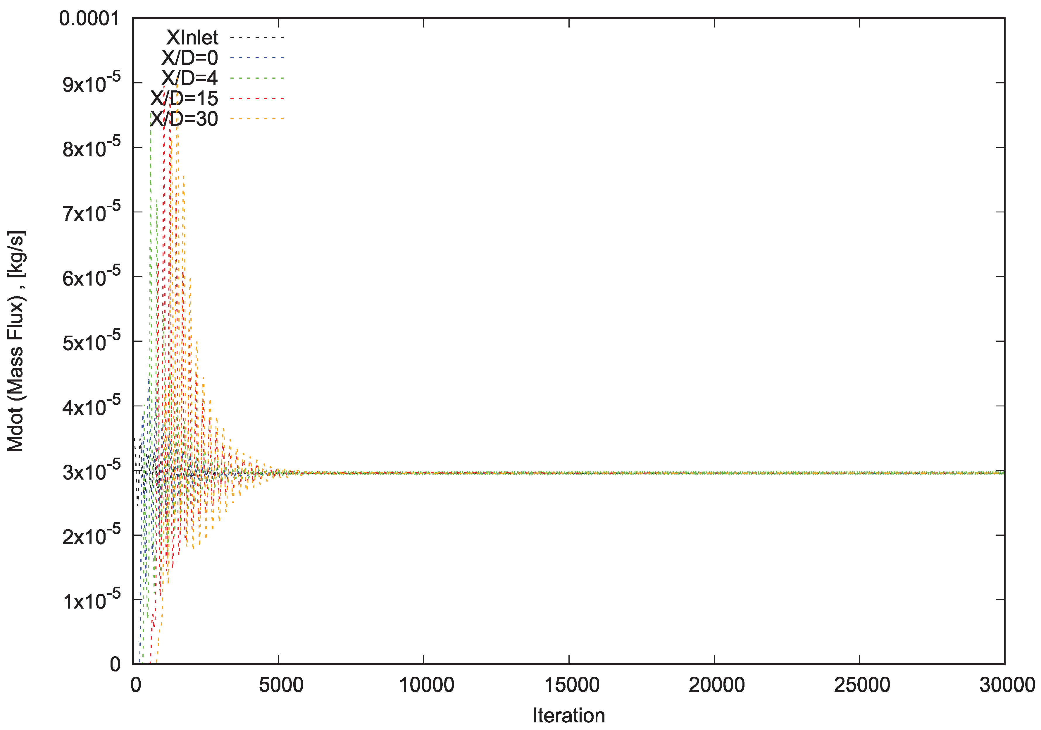
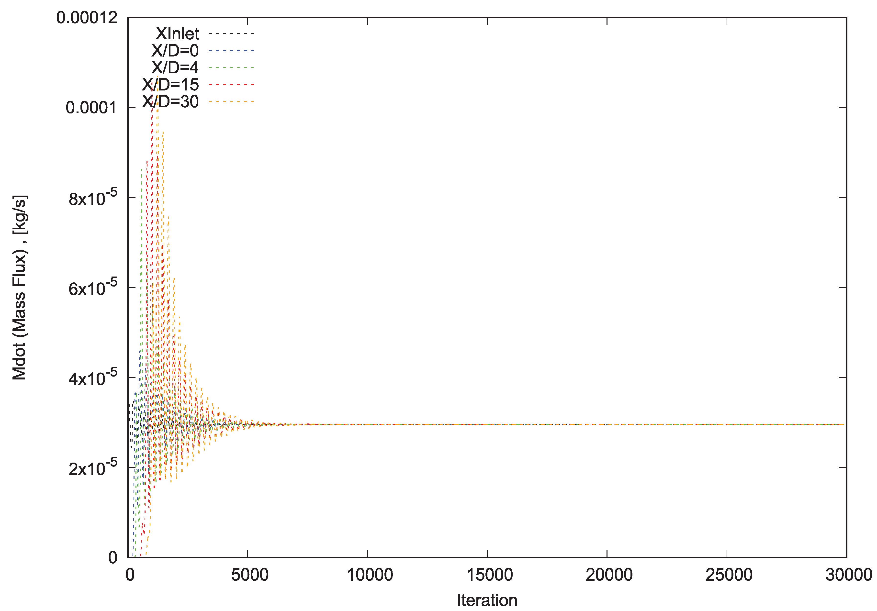
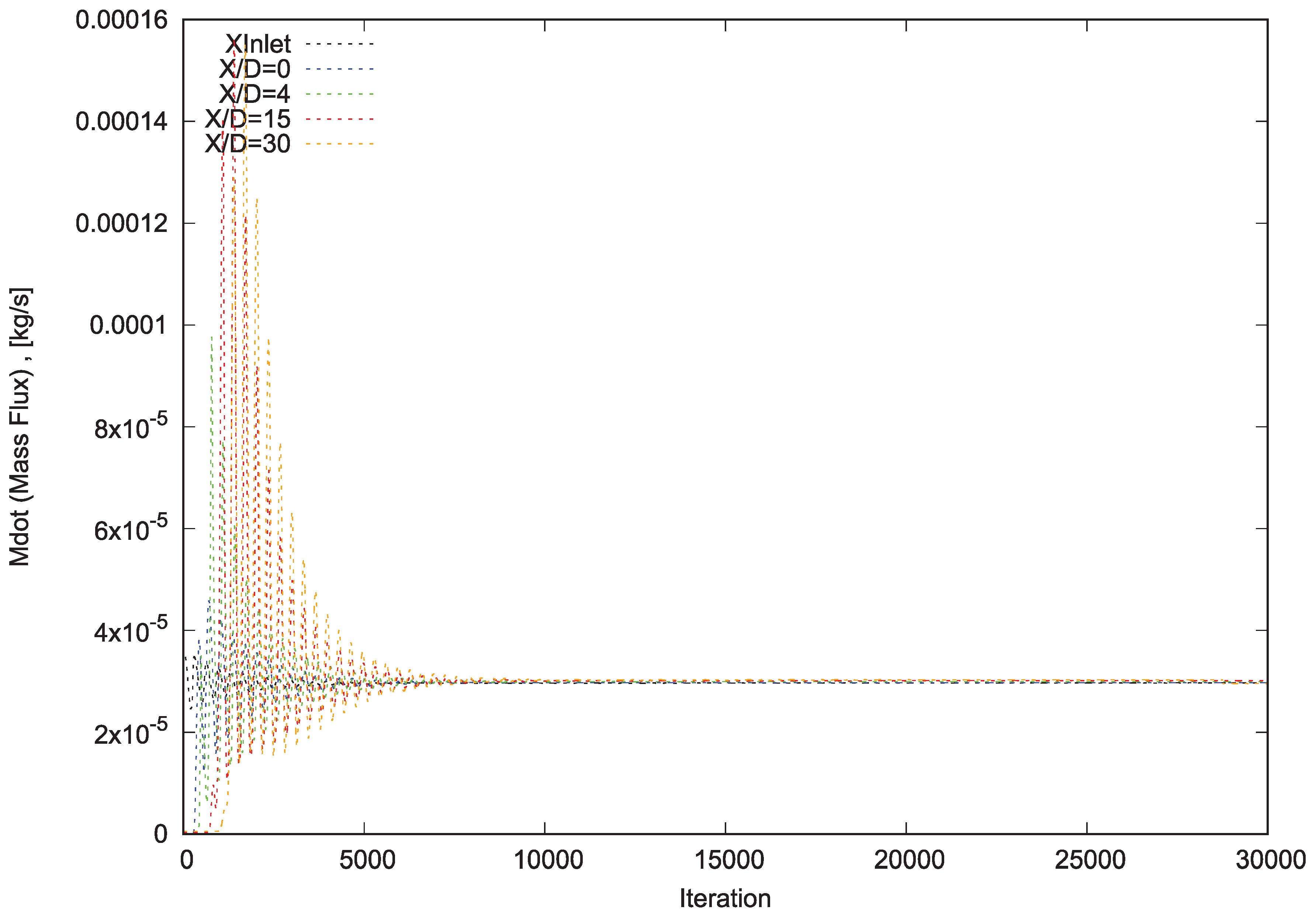
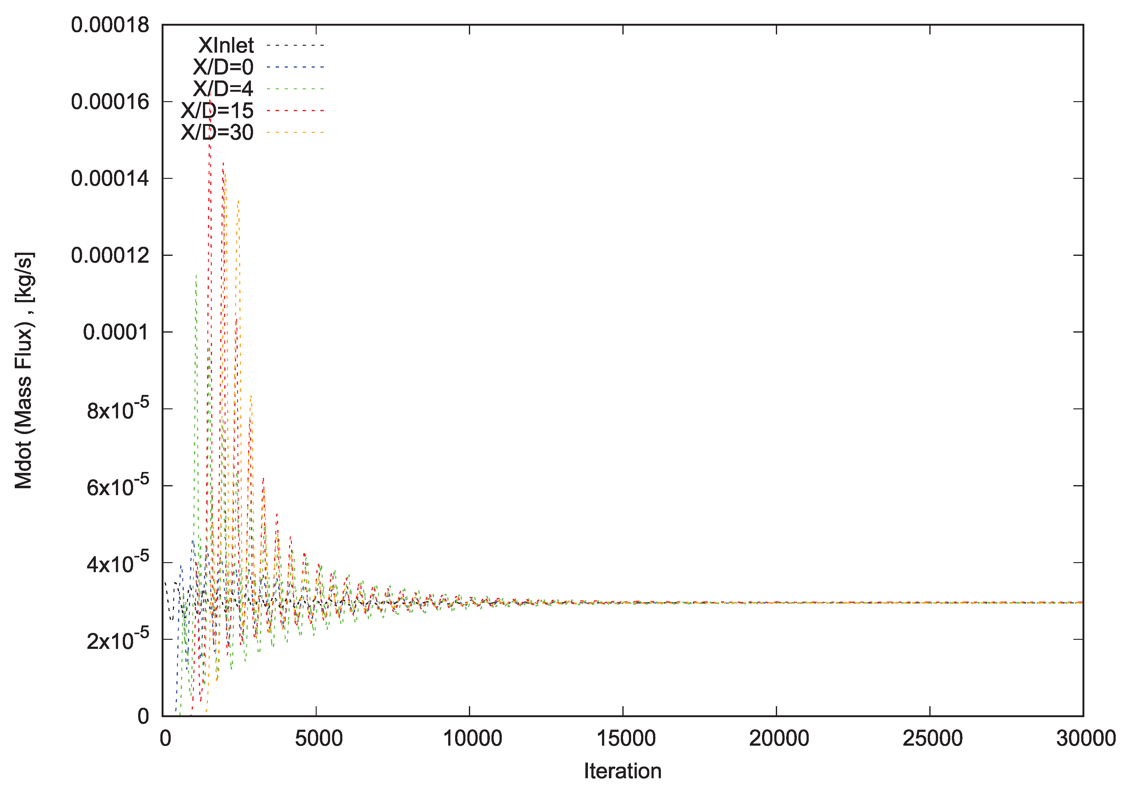
Afterward, all the tests cases have been performed for 30,000 iterations. Subsequently, the massGraph file has been plotted as massGraph.eps for each test case to investigate needed iterations for converging (Figures 2, 3, 4 and 5). Finally, the steady-state (converged) results of all test cases have been compared to each other to pick out the independent grid.

It should be noticed that all the phases of the performance for each test case have been carried out through Allrun script file, in serial mode (on single CPU), on an ordinary laptop.

To assess the accuracy of the numerical measurements, it has been observed that for each test case and on 4 reference levels (x/D=0, 4 , 15 and 30), massGraph.eps (convergence diagram of mass flux) and momentumGraph.eps (convergence diagram of total momentum) plots have revealed the convergence and conversation of Propane and conservation of total momentum.

It can be perceived that after passing sufficient requisite iterations in each test case, total mass flux of numerical domain (5 degrees sector) at all 4 reference levels, has been converged to 2.952e-02 g/s (=2.125 gr/s for total reference assumed cylinder) which is 7.6% less than measured mass flux through flow meter (2.8% less than measured mass flux by data extracted through Rayleigh Scattering System and Laser Doppler Velocimetry).

8. Results and discussions

The independent grid's converged results have been presented through relevant figures at the end of this section to abbreviate the discussion.

Table 6 comprises a detailed list of assigned discretizing schemes for various terms, which have been placed as the foundation of the discussion:

8.1. Umean

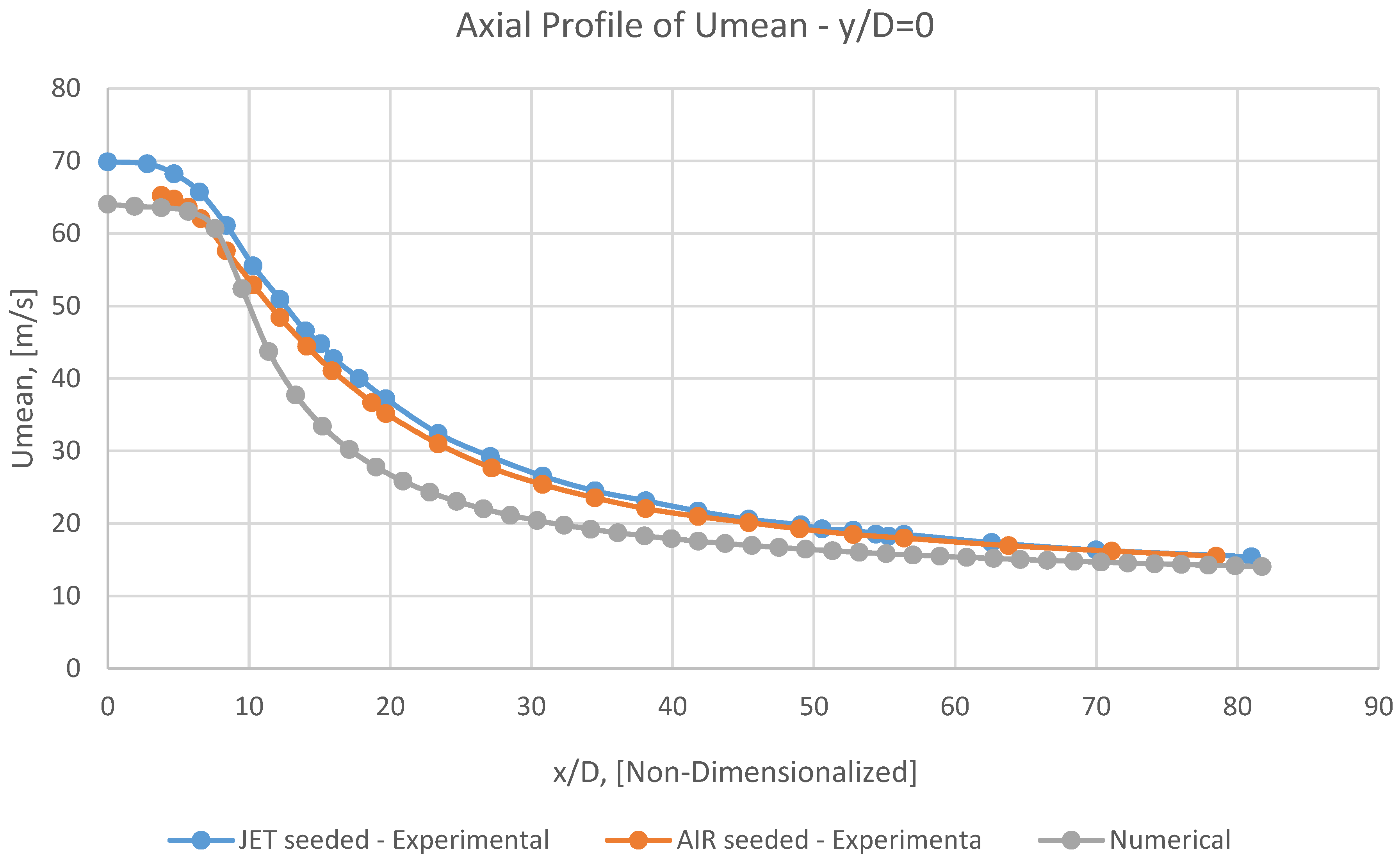
As it has been apparently demonstrated in Figure 18, due to imposing a mean uniform profile for axial velocity to the numerical model at inletfuel, the jet has been authorized to establish a fully turbulent profile while passing through the nozzle.

Consequently, at the end of the 10 cm nozzle (i.e., at the inject point) fully-developed pipe flow theory is instituted and Umean's profile has the maximum value of 64.028 m/s (7.2% less than the maximum of experimental Umean).

The numerical Umean remains nearly constant for approximately 6 jet diameters downstream of the nozzle outlet, before decreasing rapidly to approach the outer co-flowing air velocity of 9.2 m/s farther downstream.

It should be emphasized that the propellant of the mixing between injected Propane and the co-flowing air is nothing but turbulence which is due to vorticities.

The transport equation of the aforementioned vorticities has a source term which involves the gradient of the mean velocities.

Accordingly, these vorticities (and consequently, the turbulence and the mixing from there), will be intensified where the gradients of velocities are more augmented.

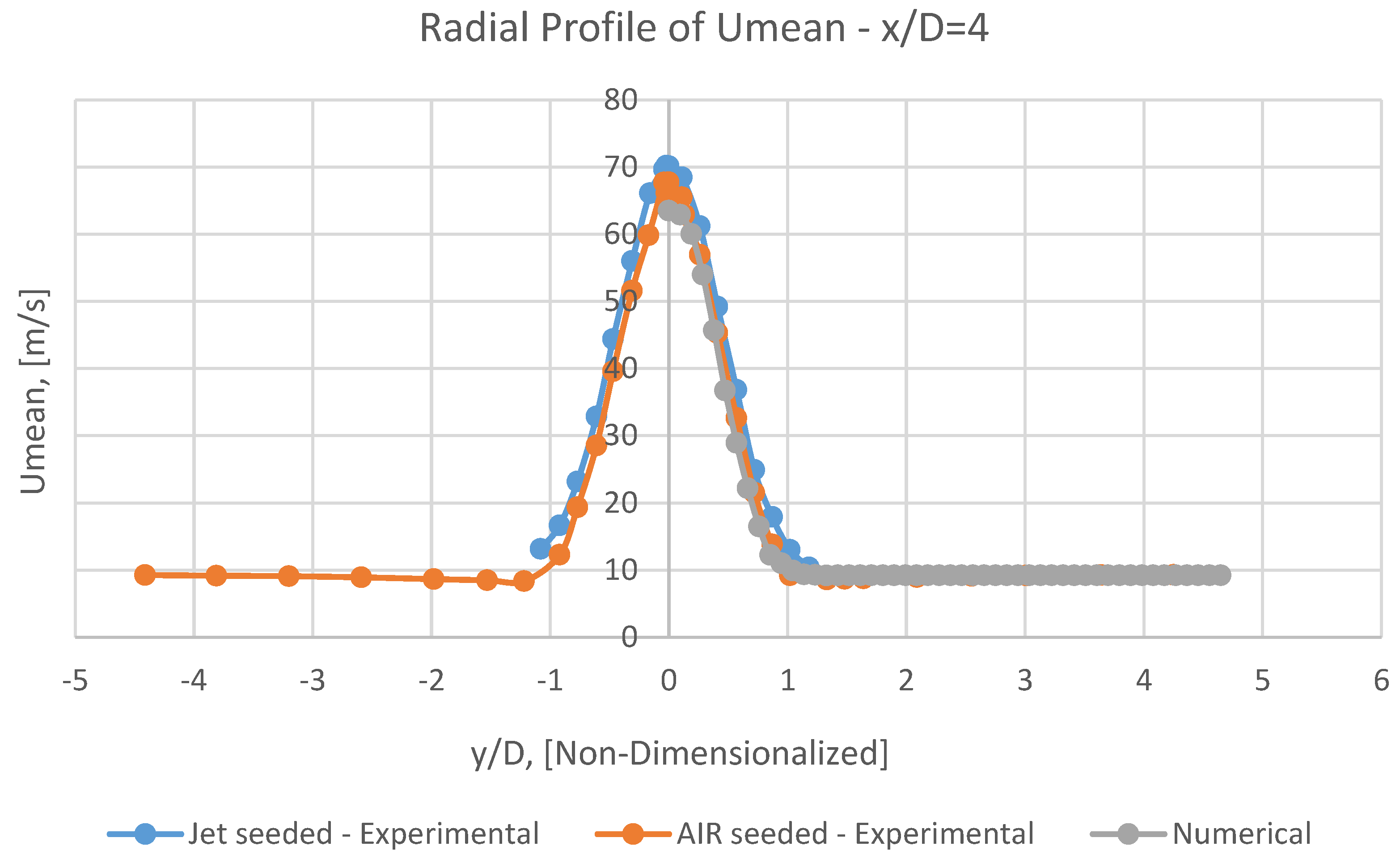
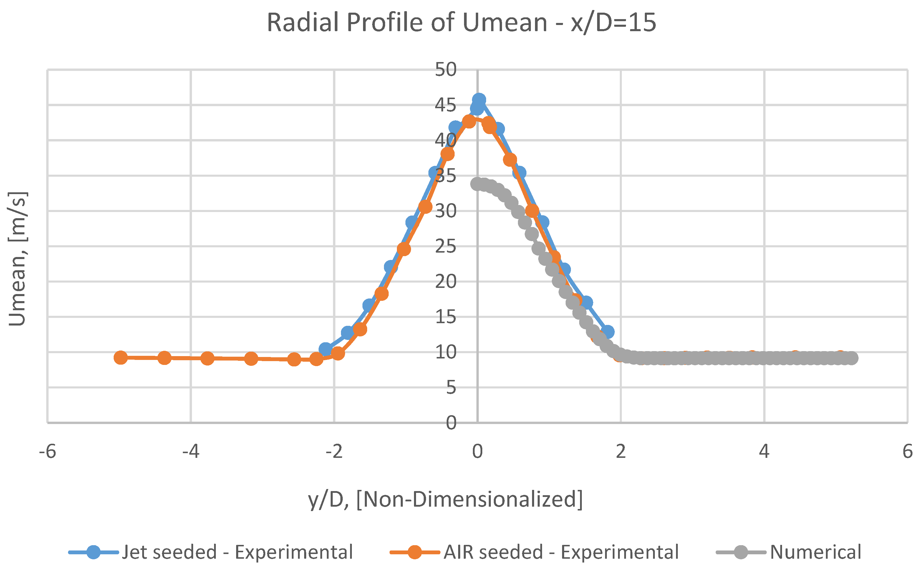
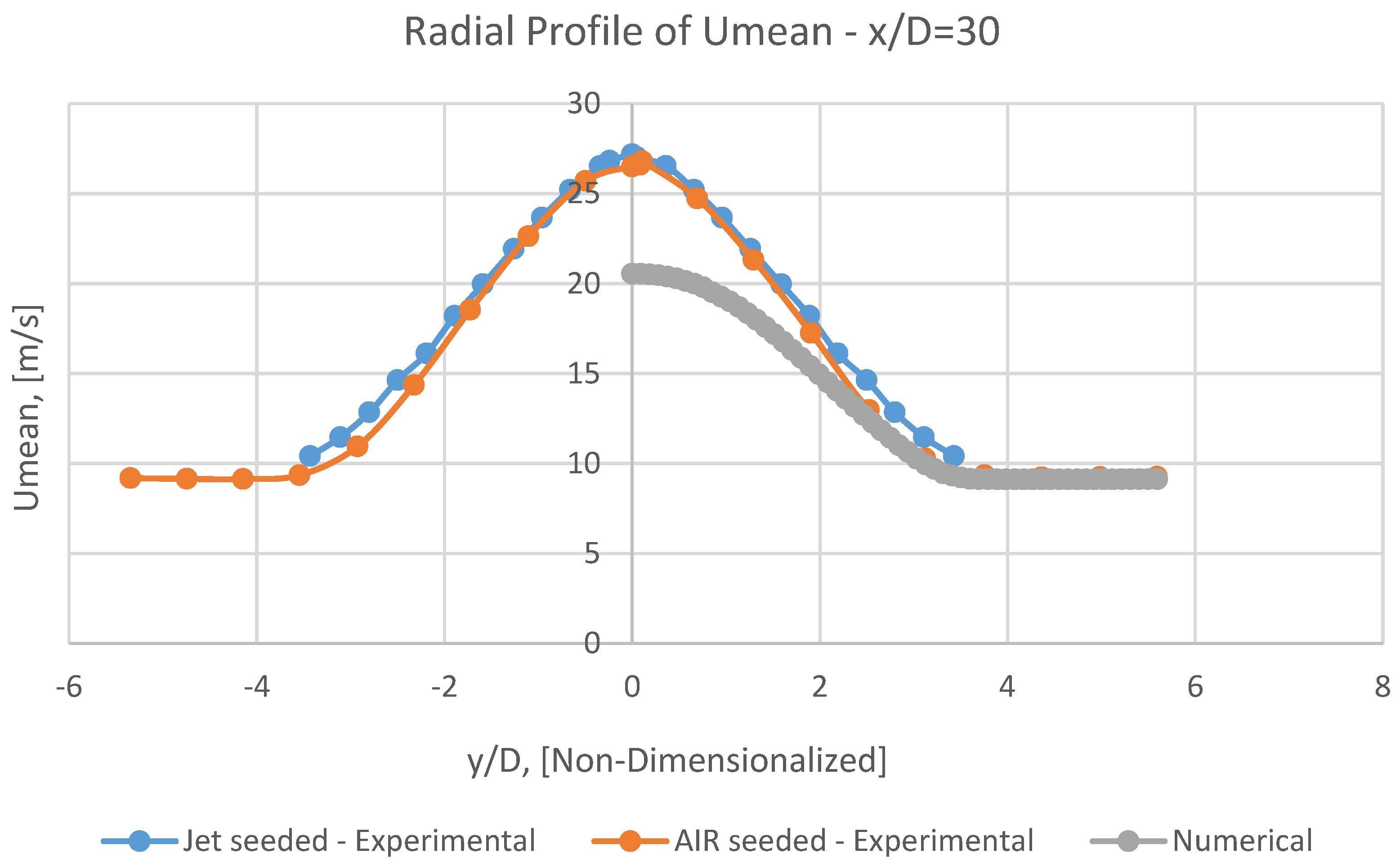
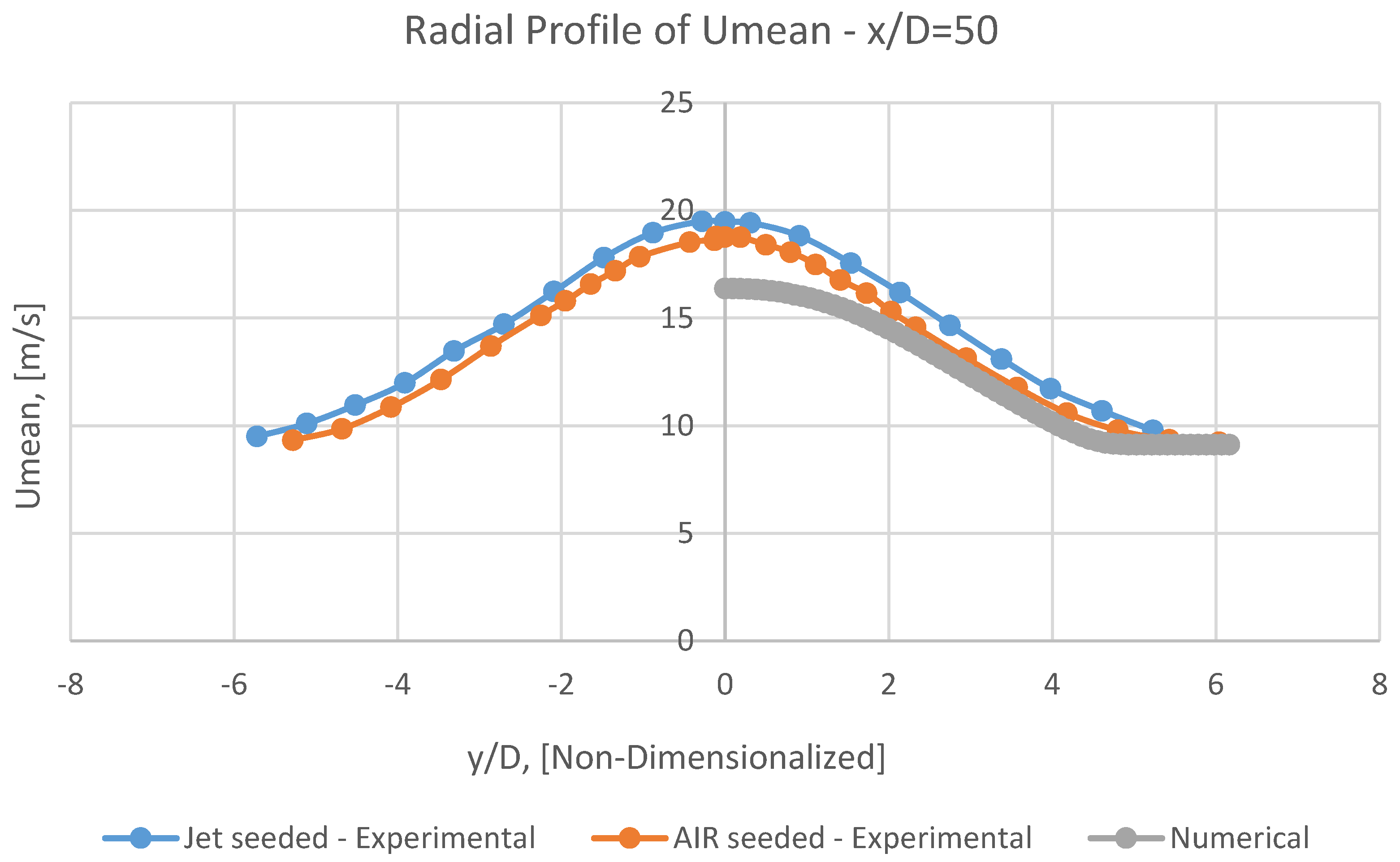
It can be perceivable from Figures 18, 20, 21, 22 and 23 that at first, the radial profile of numerical Umean has a superb adaptation with corresponding experimental data in the vicinity of the jet (i.e., in x/D<10).

But subsequently, having marched toward the outlet, this conformity will be gradually diminished (i.e., in 10<x/D<30).

Eventually, this coincidence will be revitalized and be radiantly improved (i.e., in x/D>30).

It should be kept in mind that each radial distance, y, is normalized by the inner diameter of the nozzle, D.

In numerical mean radial profiles of Umean (Figures 20, 21, 22 and 23), it is observable that at increasing radial distances, although the mean velocities rapidly approach free stream values of 9.2 m/s, the rate of this acceding will be pacified.

It should be accentuated that this behavior of velocity is similar than demeanor of Mixed Fraction of Propane in L_f's diagram (Figure 6), i.e., having receded from the nozzle, the width of the jet will be gently expanded.

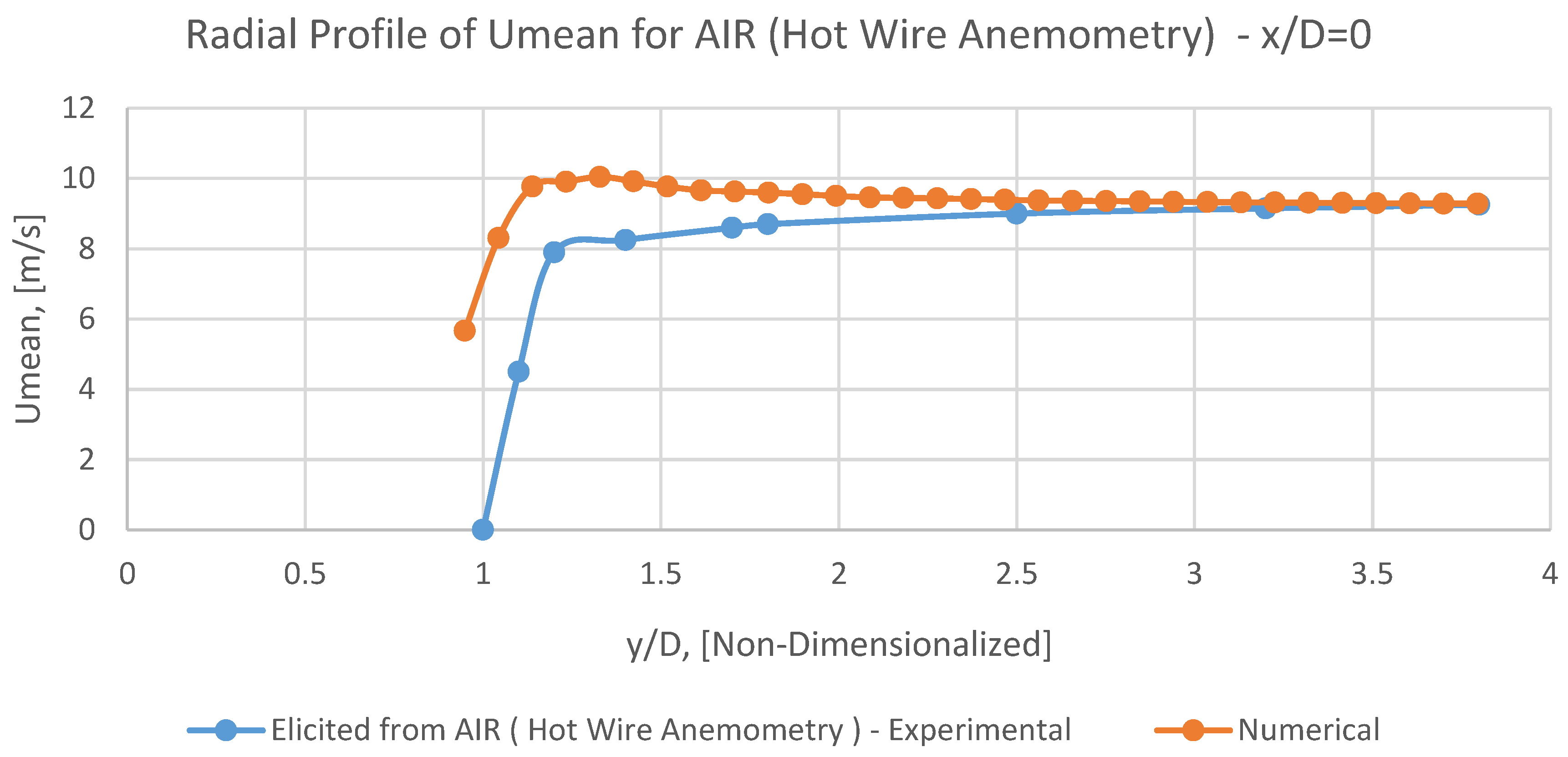
Finally, in radial profile of Umean at x/D=0, (Figure 19), it can be noticed that the numerical results are in an eligible conform with corresponding experimental data, especially from the outer diameter of the nozzle (i.e., y/D=1.7) toward the leftside boundary.

8.2. Vmean

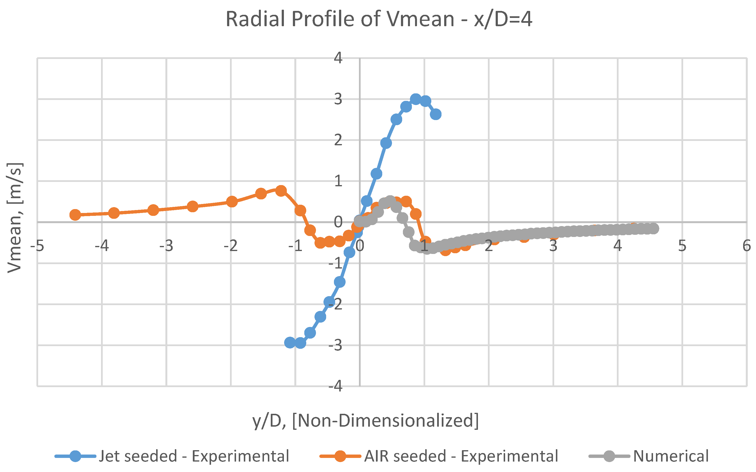
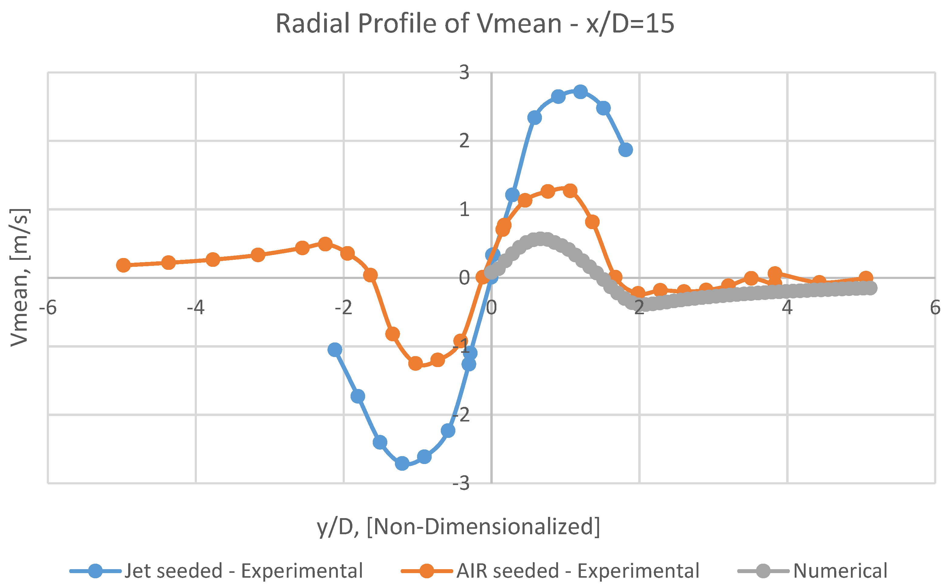
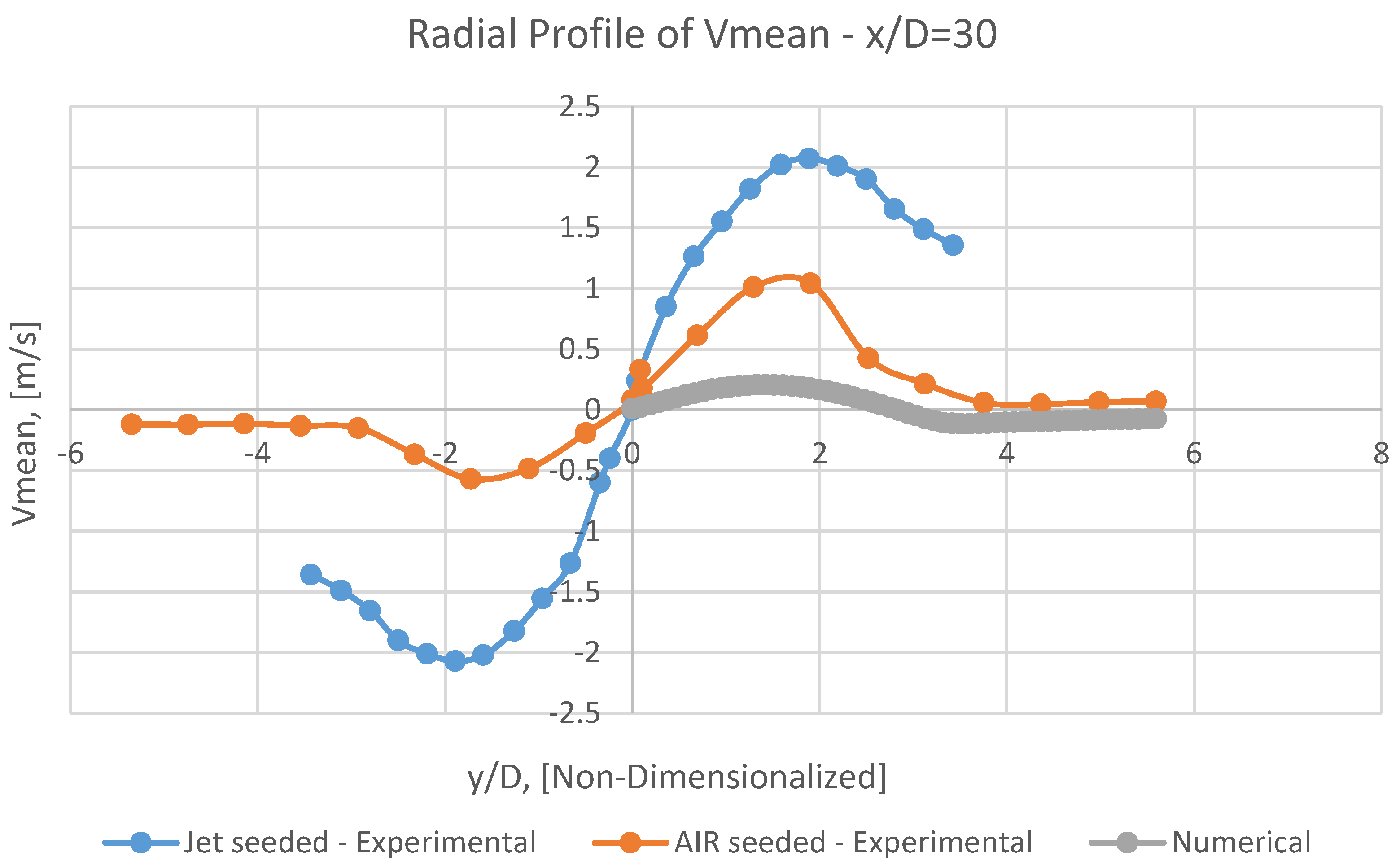
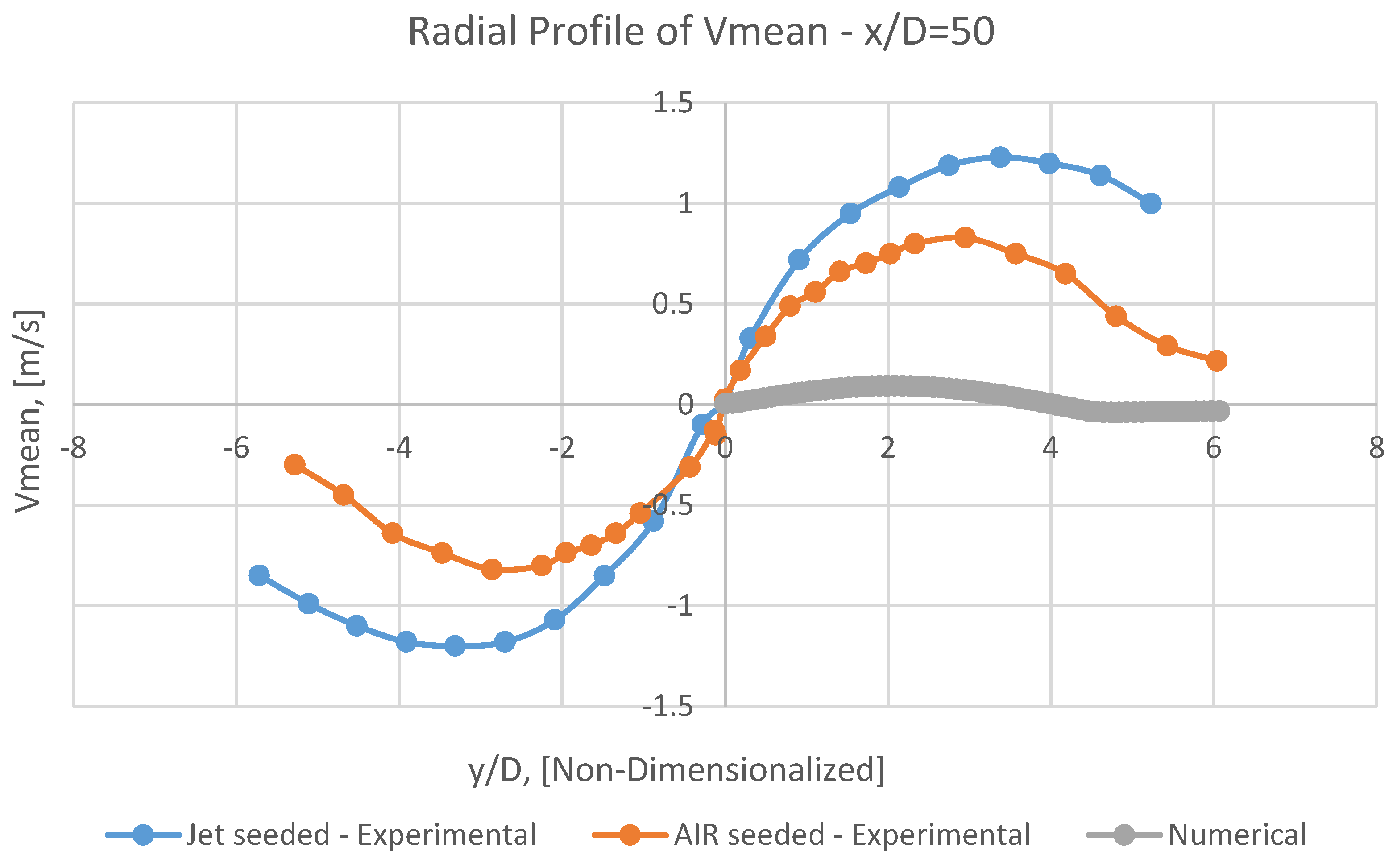
It can be perceivable from Figures 25, 26, 27 and 28, the numerical Vmean has a conceptual adaptation with both AIR seeded experimental results, and the corresponding JET seeded data.

However, having approached toward the outlet, the scale of this conformity will be leniently assuaged.

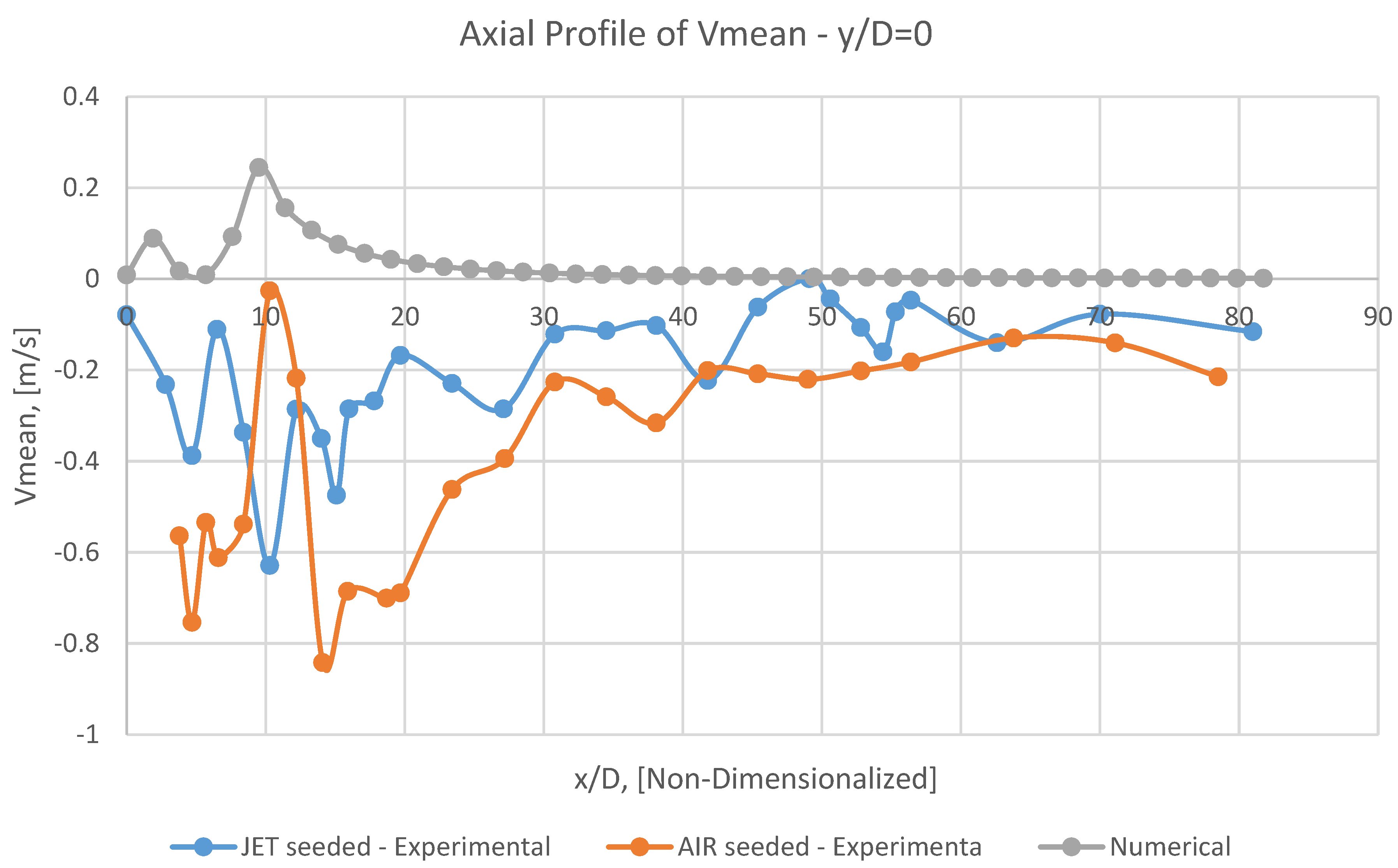
Unfortunately, in the axial profile of Vmean at y/D=0 (Figure 24), it is not conceivable to attain a logical coincidence between numerical results and experimental ones.

It may be caused by debilities of RANS models in such problem, or by excessive simplification of the problem by assumptions as mentioned earlier in the present numerical model.

It should be emphasized that capturing radial velocity (Vmean) seems to be frequently so demanding, even with more sophisticated models, for example, LES [29].

8.3. Turbulence Kinetic Energy (k)

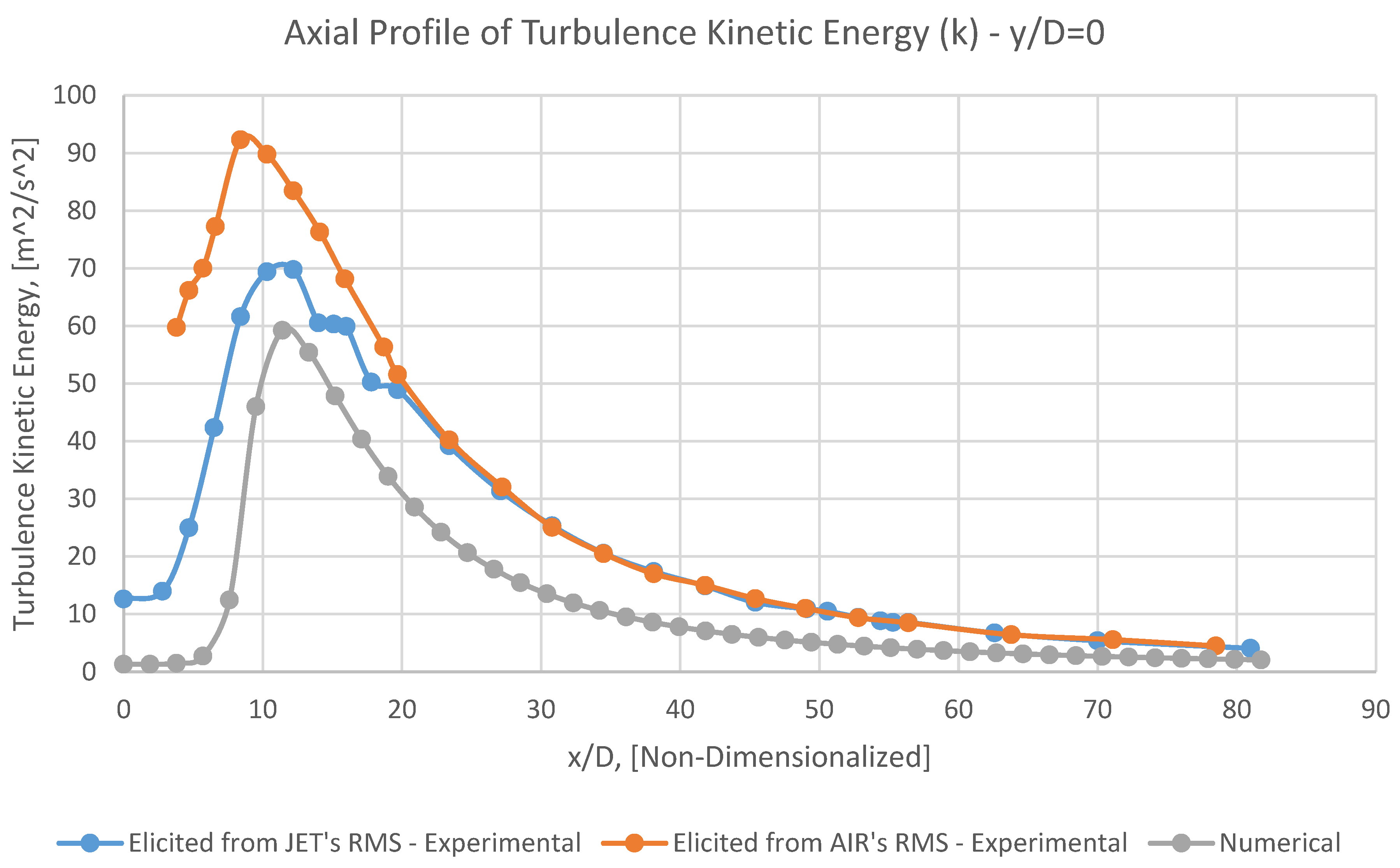
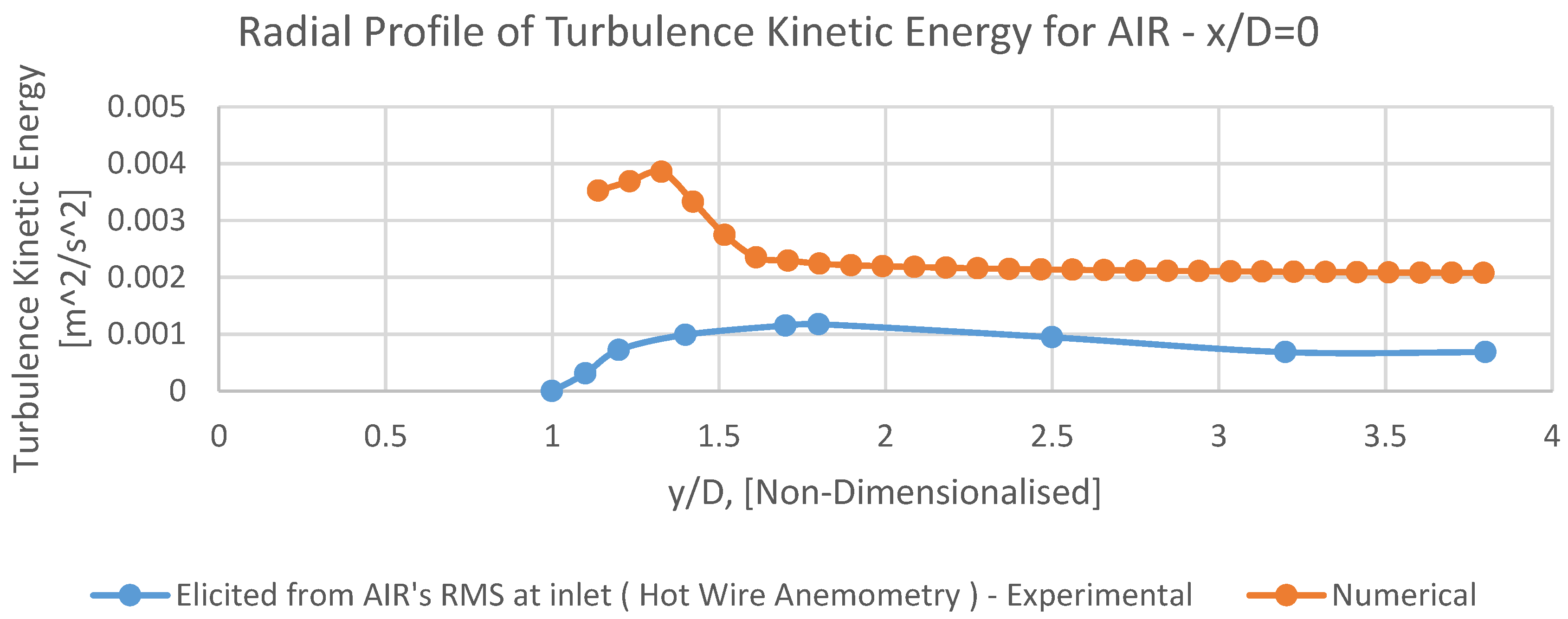
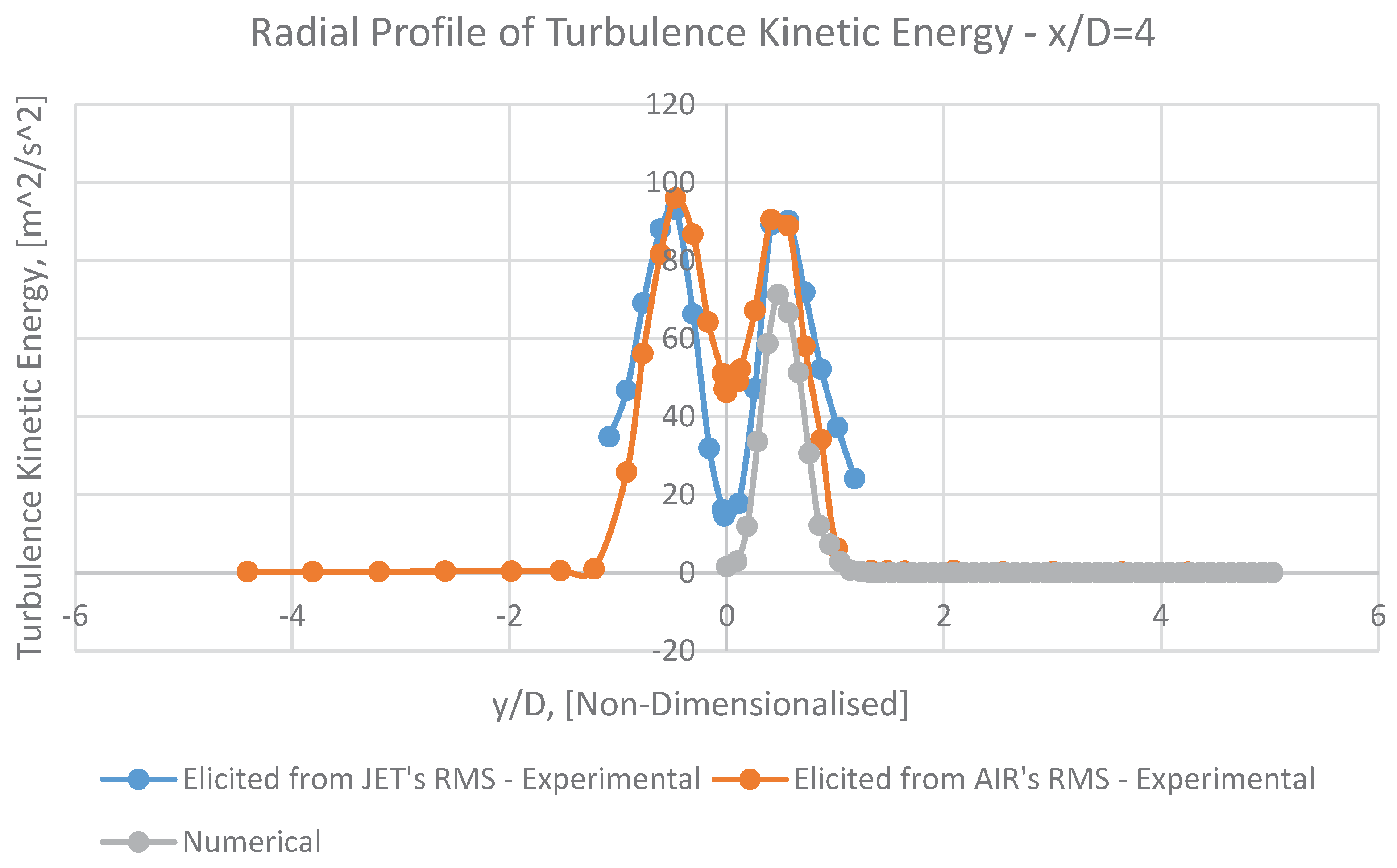
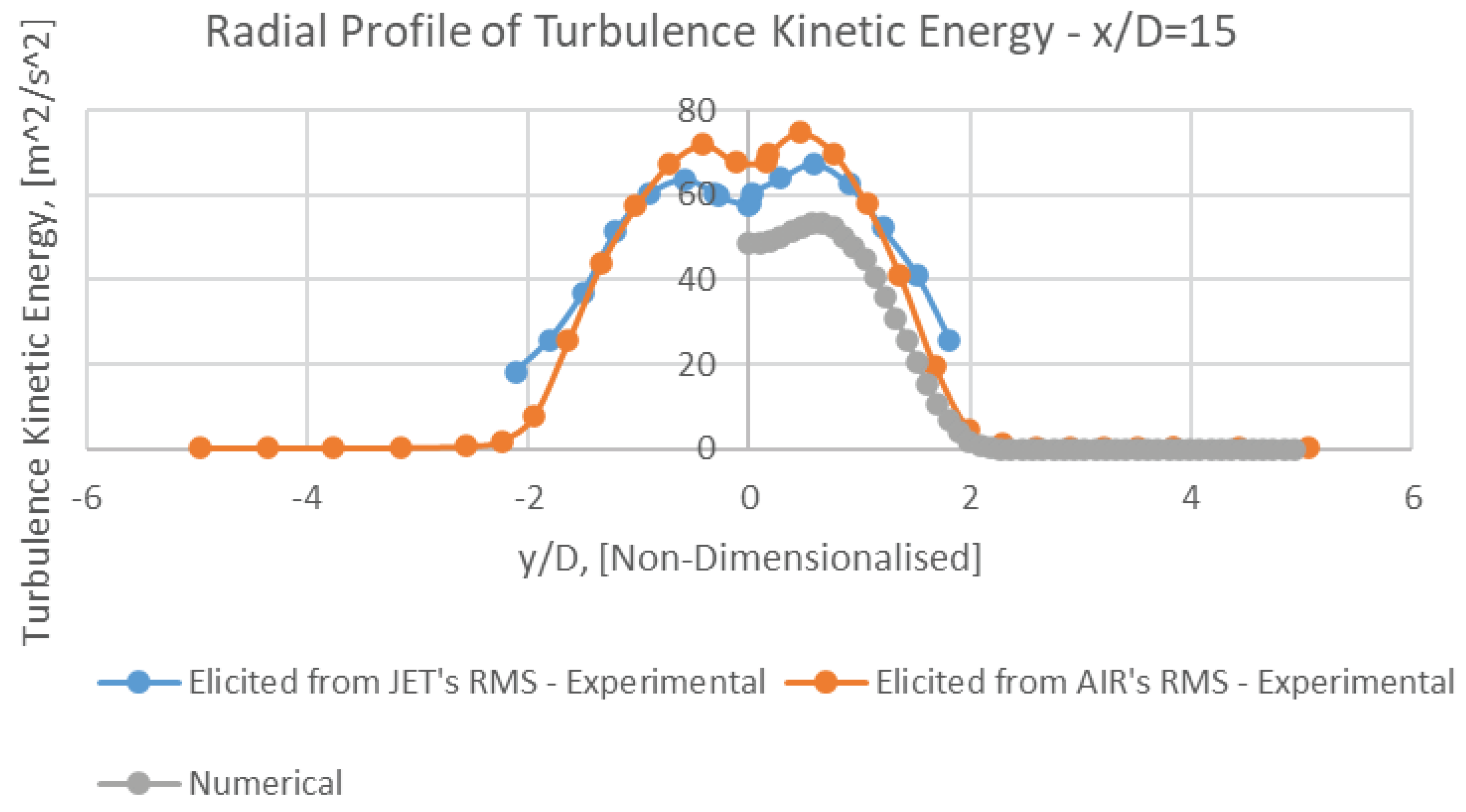
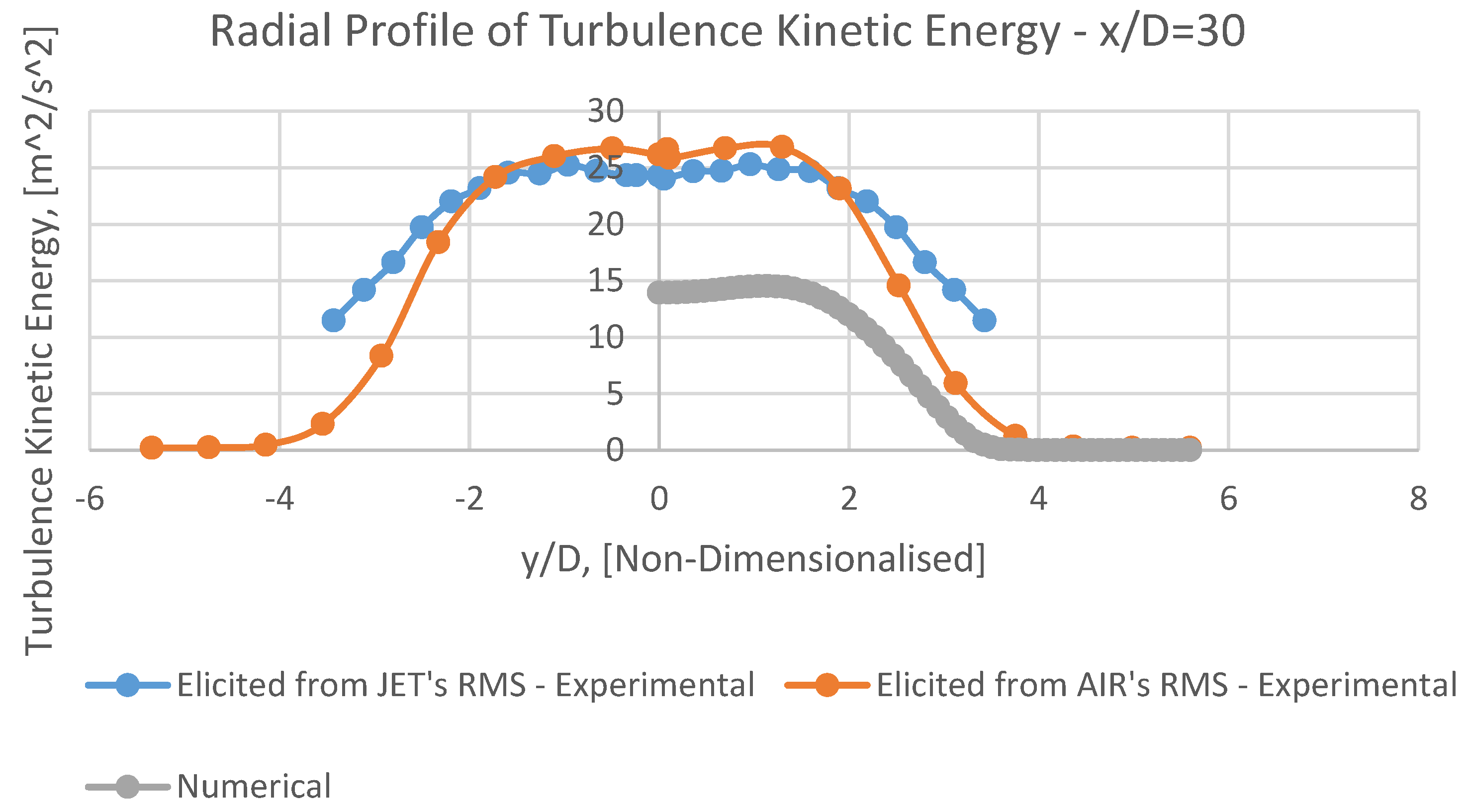
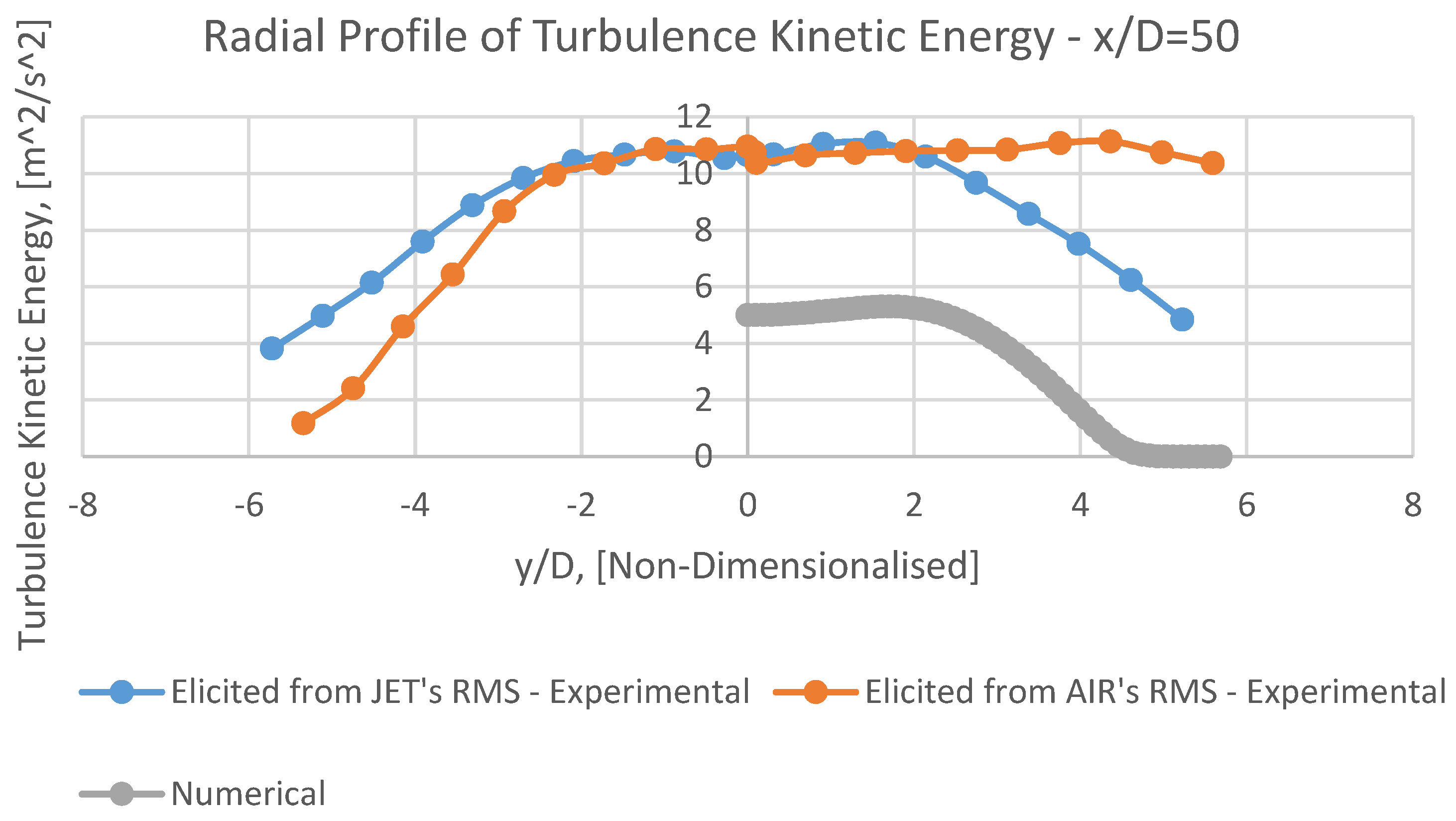
It can be perceivable from Figures 12, 14, 15, 16 and 17 that the radial profiles of turbulence kinetic energy (k) have an appropriate overall adaptation with corresponding experimental data.

Having approached toward the outlet, this conformity will be gradually improved, due to alleviated fluctuations of velocity. (approximately after x/D<50).

In numerical mean radial profiles of k (Figures 14, 15, 16 and 17), it is observable that at increasing radial distances, the mean turbulence kinetic energy, k, will be gradually alleviated.

Again, as like as Umean, having receded from the nozzle, the width of the jet will be steadily expanded, which is conform with the manner of Mixed Fraction of Propane in L_f's diagram(Figure 6).

Eventually, in radial profile of turbulence kinetic energy, k, at x/D=0, (Figure 13), as like as Umean it can be noticed that the numerical results are in a good adaptation with corresponding experimental data, especially from the outer diameter of the nozzle (i.e., y/D=1.7) toward the leftside boundary.

8.4. Mixture Fraction of Propane

Due to technical problems of corresponding experiments, it is not conceivable to elicit experimental data of Propane's mean mixture fraction at the inlet (i.e., x/d=0).

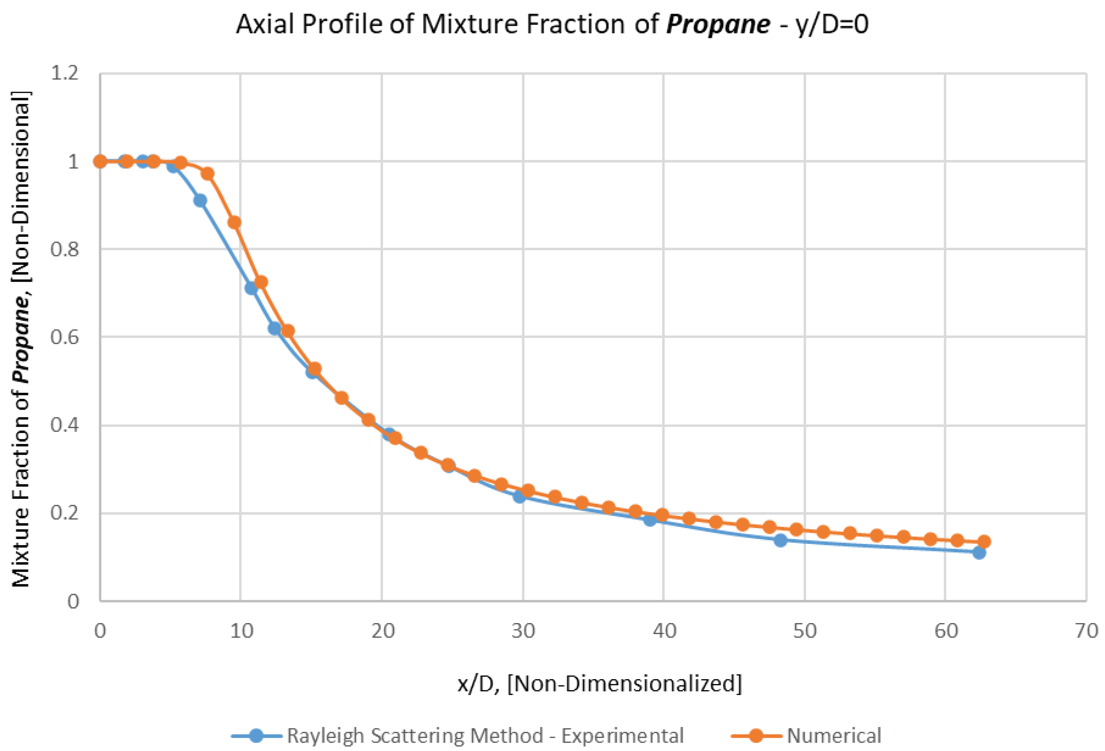
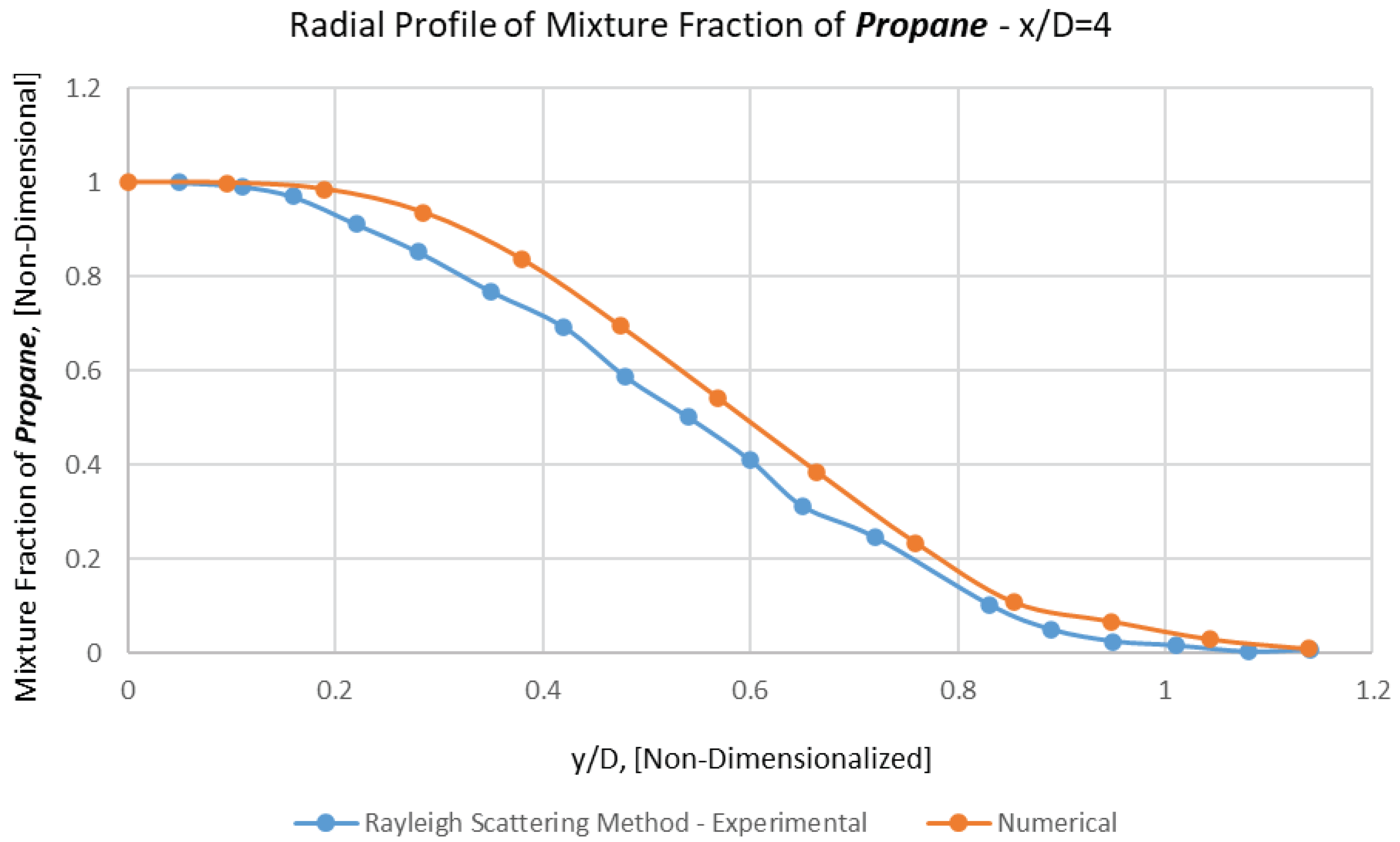
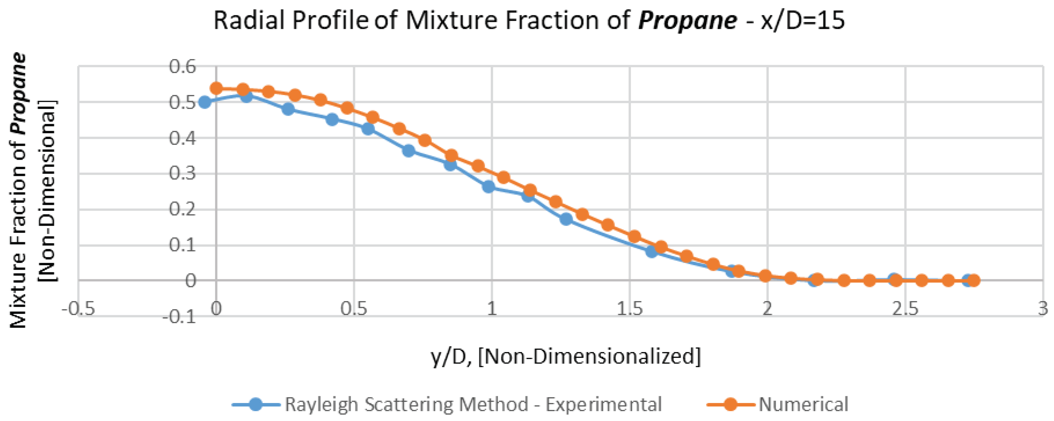
Thus, corresponding axial and all the radial comparisons have been carried out at x/D=4, 15, 30, 50 (Figures 6, 7, 8, 9, 10 and 11).

As it is manifestly observable in these figures, a magnificent conformation between numerical results and experimental data have been revealed in the sphere of mean mixture fraction and its half radius (L_f), either for axial profile or radial ones.

It should be noticed that in numerical results at x/D=4, the mean mixture fraction values of unity (corresponding to pure Propane) announces the existence of a potential core, which extends approximately 0.2 diameters from the centerline.

The numerical mean mixture fraction remains approximately constant over this potential core region, which extends nearly 6 jet diameters downstream of the nozzle's outlet, before drastically decreasing due to co-flowing air is entrained because of Kelvin-Helmholtz instabilities (due to drastic difference between Jet's and air's velocities).

8.5. Mixture Fraction Half Radius (L_f)

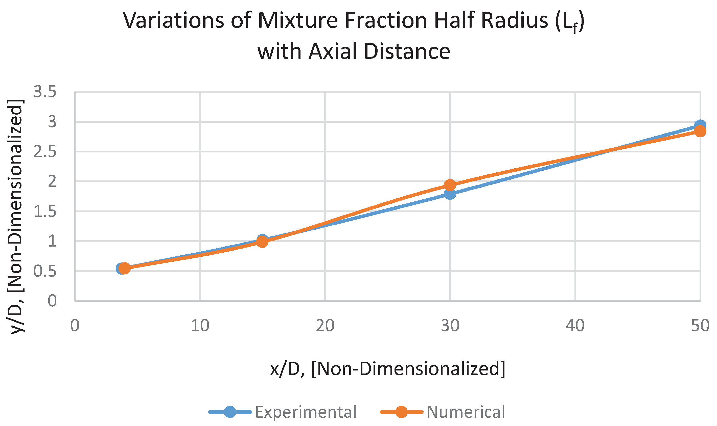
L_f, ascertains the jet spreading rate, would be defined as the radial location at which the mixture fraction is equal to half its value at the centerline. Figure 11, shows the variations of mixture fraction half radius, L_f, (normalized by D) with axial distance. It is explicit that it reveals a phenomenal conformity with the corresponding experimental data.

9. Conclusion

Having manipulated reactingFoam (one of the standard solvers in OpenFOAM) through eliminating reaction and combustion, some numerical simulation of velocity and mixture fraction fields have been carried out in a turbulent non-reaction Propane jet flow issuing into parallel co-flowing air, in isothermal condition, and compared with experimental data which had been previously described here: http://www.sandia.gov/TNF/DataArch/ProJet.html.

In this regard, a two-equation Realizable k-ε eddy viscosity turbulence model has been used to simulate the turbulent flow field on a 2D plane (i.e., on a 5-degree sector of the experimental domain) to attain a better understanding of the flow structure and mixing process in a situation which there is no chemical interaction and heat-transfer.

Having compared the elicited numerical axial and radial profiles of mean velocities, turbulence energy, mean mixture fraction, and the mixture fraction half radius (L_f) with corresponding experimental data, superb conformations have been revealed for mixture fraction fields and mixture fraction half radius (L_f). Moreover, in contrast with Vmean, it has been relatively observed appropriate adaptations for Umean, especially when the investigated areas had been inclined toward the nozzle exit.

Altogether, regarding the extreme shortened numerical expenditures (due to the significant simplifying assumption in both test cases' diverse adjustments and turbulence model) in comparison with more sophisticated turbulence models (for example LRR, SSG, DES, LES, and so on), the elicited numerical results have eminently demonstrated relevant precisions and conformity with the experimental data in aforesaid spheres.

Figure 2. Convergence Diagram of Mass Flux for Mesh A.

Figure 3. Convergence Diagram of Mass Flux for Mesh B.

Figure 4. Convergence Diagram of Mass Flux for Mesh C.

Figure 5. Convergence Diagram of Mass Flux for Mesh D.

Figure 6.

Figure 7.

Figure 8.

Figure 9.

Figure 10.

Figure 11.

Figure 12.

Figure 13.

Figure 14.

Figure 15.

Figure 16.

Figure 17.

Figure 18.

Figure 19.

Figure 20.

Figure 21.

Figure 22.

Figure 23.

Figure 24.

Figure 25.

Figure 26.

Figure 27.

Figure 28.

References

Kannan, B. , Computation of an axisymmetric jet using OpenFOAM. Procedia Engineering, 2015. 127: p. 1292-1299. [CrossRef]
Imine, B.; Imine, O.; Abidat, M.; Liazid, A. Study of non-reactive isothermal turbulent asymmetric jet with variable density. Comput. Mech. 2005, 38, 151–162. [Google Scholar] [CrossRef]
Schefer, R. and R. Dibble, Mixture fraction field in a turbulent nonreacting propane jet. AIAA journal, 2001. 39(1): p. 64-72. [CrossRef]
Yanagi, T.; Mimura, Y. Velocity-temperature correlation in premixed flame. Symp. (International) Combust. 1981, 18, 1031–1039. [Google Scholar] [CrossRef]
Moss, J.B. Simultaneous Measurements of Concentration and Velocity in an Open Premixed Turbulent Flame. Combust. Sci. Technol. 1980, 22, 119–129. [Google Scholar] [CrossRef]
Driscoll, J., R. Schefer, and R. Dibble. Mass fluxes ρ′ u′¯ and ρ′ υ′¯ measured in a turbulent nonpremixed flame. in Symposium (International) on Combustion. 1982. Elsevier.
Wygnanski, I.; Fiedler, H. Some measurements in the self-preserving jet. J. Fluid Mech. 1969, 38, 577–612. [Google Scholar] [CrossRef]
Becker, H.A.; Hottel, H.C.; Williams, G.C. The nozzle-fluid concentration field of the round, turbulent, free jet. J. Fluid Mech. 1967, 30, 285–303. [Google Scholar] [CrossRef]
Shaughnessy, E.J.; Morton, J.B. Laser light-scattering measurements of particle concentration in a turbulent jet. J. Fluid Mech. 1977, 80, 129–148. [Google Scholar] [CrossRef]
Dowling, D.R.; Lang, D.B.; Dimotakis, P.E. An improved laser-Rayleigh scattering photodetection system. Exp. Fluids 1989, 7, 435–440. [Google Scholar] [CrossRef]
Dowling, D.R.; Dimotakis, P.E. Similarity of the concentration field of gas-phase turbulent jets. J. Fluid Mech. 1990, 218, 109–141. [Google Scholar] [CrossRef]
Fulachier, L., F. Anselmet, and M. Amielh, Turbulent jets with variable density, PRC combustion in the rocket motors cryotechnic. 1990, CNRS/CNES/SEF.
Gazzah, M.H. , et al., Simulation numérique des jets turbulents subsoniques à masse volumique variable par le modèle k–ε. International journal of thermal sciences, 2002. 41(1): p. 51-62. [CrossRef]
Gouldin, F. , et al., Nonreacting turbulent mixing flows. Progress in energy and combustion science, 1986. 12(4): p. 257-303. [CrossRef]
Panchapakesan, N.R.; Lumley, J.L. Turbulence measurements in axisymmetric jets of air and helium. Part 1. Air jet. J. Fluid Mech. 1993, 246, 197–223. [Google Scholar] [CrossRef]
Panchapakesan, N.R.; Lumley, J.L. Turbulence measurements in axisymmetric jets of air and helium. Part 2. Helium jet. J. Fluid Mech. 1993, 246, 225–247. [Google Scholar] [CrossRef]
Pietri, L.; Amielh, M.; Anselmet, F. Simultaneous measurements of temperature and velocity fluctuations in a slightly heated jet combining a cold wire and Laser Doppler Anemometry. Int. J. Heat Fluid Flow 2000, 21, 22–36. [Google Scholar] [CrossRef]
Purwanto, A. , Modélisation d'écoulements turbulents-basse vitesse à forte variation de masse volumique: application aux schémas de fermeture kappa-epsilon. 1994, Toulouse, INPT.
So, R.M.C.; Zhu, J.Y.; Ötügen, M.V.; Hwang, B.C. Some measurements in a binary gas jet. Exp. Fluids 1990, 9, 273–284. [Google Scholar] [CrossRef]
Thring, M.; Newby, M. Combustion length of enclosed turbulent jet flames. Symp. (International) Combust. 1953, 4, 789–796. [Google Scholar] [CrossRef]
Stårner, S.H.; Bilger, R.W.; Dibble, R.W.; Barlow, R.S. Piloted Diffusion Flames of Diluted Methane Near Extinction: Mean Structure from Raman/Rayleigh Fluorescence Measurements. Combust. Sci. Technol. 1990, 70, 111–133. [Google Scholar] [CrossRef]
Meier, W. , et al., Simultaneous Raman/LIF measurements of major species and NO in turbulent H 2/air diffusion flames. Applied Physics B, 1996. 63(1): p. 79-90. [CrossRef]
Weller, H.G.; Tabor, G.; Jasak, H.; Fureby, C. A tensorial approach to computational continuum mechanics using object-oriented techniques. Comput. Phys. 1998, 12, 620–631. [Google Scholar] [CrossRef]
Mhiri, H. , et al., Etude numérique des conditions d'émission sur un écoulement de type jet plan turbulent isotherme ou chauffé. International journal of thermal sciences, 1999. 38(10): p. 904-915. [CrossRef]
Fluent, A. , ANSYS fluent theory guide 15.0. ANSYS, Canonsburg, PA, 2013.
Versteeg, H.K. and W. Malalasekera, An introduction to computational fluid dynamics: the finite volume method. 2007: Pearson education.
Shih, T.-H.; Liou, W.W.; Shabbir, A.; Yang, Z.; Zhu, J. A new k-ϵ eddy viscosity model for high reynolds number turbulent flows. Comput. Fluids 1995, 24, 227–238. [Google Scholar] [CrossRef]
Marzouk, O.A. and E.D. Huckaby, Simulation of a Swirling Gas-Particle Flow Using Different k-epsilon Models and Particle-Parcel Relationships. Engineering Letters, 2010. 18(1).
Nebenführ, B. , OpenFOAM: A tool for predicting automotive relevant flow fields. 2010. [Google Scholar]
Riber, E.; Moureau, V.; García, M.; Poinsot, T.; Simonin, O. Evaluation of numerical strategies for large eddy simulation of particulate two-phase recirculating flows. J. Comput. Phys. 2009, 228, 539–564. [Google Scholar] [CrossRef]

Figure 1. computational domain's simplified scheme.

Table 1. list of computational domain's dimensions and some inlet data.

Orientation	Vertical
Inner Diameter of the Nozzle (D/2)	(0.52)/2 cm
Outer Diameter of the Nozzle	(0.90)/2 cm
The Length of the Domain	100 cm
The Width of the Domain	30/2 cm
Propane Jet's Bulk Velocity	53 m/s
Propane Jet's Temperature	294 K
Co-flowing Air's Velocity	9.2 m/s
Co-flowing Air's Temperature	294 K
Reynolds Number (based on D)	68,000 (68,168 in velstat files)
Co-flowing Air's Turbulence Intensity	0.4%

Table 2. Brief list of initial and boundary conditions for diverse variables for the first approach.

variable	inletfuel	inletair	outlet
alphat	calculated	calculated	calculated
C3H8	fixedValue (=1.0)	fixedValue (=0.0)	inletOutlet
epsilon	turbulentMixingLenghtDissipationRateInlet	turbulentMixingLenghtDissipationRateInlet	inletOutlet
k	turbulentIntensityKineticEnergyInlet	turbulentIntensityKineticEnergyInlet	inletOutlet
N2	fixedValue (=0.0)	fixedValue (=0.763149)	inletOutlet
nut	calculated	calculated	calculated
O2	fixedValue (=0.0)	fixedValue (=0.236851)	inletOutlet
p	zeroGradient	zeroGradient	totalPressure
T	fixedValue (=294)	fixedValue (=294)	inletOutlet
U	fixedValue (=53)	fixedValue (=9.2)	pressureInletOutletVelocity

Table 3. Brief list of initial and boundary conditions for diverse variables for the first approach.

variable	leftside	burnerwall	internalField
alphat	zeroGradient	Compressible::alphatWallFunction	0
C3H8	zeroGradient	zeroGradient	0
epsilon	zeroGradient	epsilonWallFunction	200
k	zeroGradient	kqWallFunction	1
N2	zeroGradient	zeroGradient	0.7632
nut	zeroGradient	nutkWallFunction	0
O2	ZeroGradient	zeroGradient	0.2368
p	zeroGradient	zeroGradient	101325
T	zeroGradient	zeroGradient	294
U	fixedValue (=9.2)	fixedValue (=0.0)	9.2

Table 4. list of assigned discretizing schemes for diverse terms.

terms	schemes
ddtSchemes	localEuler
gradSchemes	GaussLinear
div(phi,U)	Gauss limitedLinearV 1
div(phi,Yi)	Gauss limitedLinear01 1
div(phi,h)	Gauss limitedLinear 1
div(phi,k)	Gauss limitedLinear 1
div(phi,p)	Gauss limitedLinear 1
div(phi,epsilon)	Gauss limitedLinear 1
div(phi,Yi_h)	Gauss limitedLinear01 1
div(phi,k)	Gauss limitedLinear 1
div(((rhonuEff)dev2(T(grad(U)))))	Gauss linear
laplacianSchemes	Gauss linear orthogonal
interpolationSchemes	linear
snGradSchemes	orthogonal

Table 5. Numerical details of diverse meshes.

Mesh	Number of Cells	Max. Aspect Ratio	Max. Skewness	Non-Orthogonality	Converged at about (iteration)	Needed Time (h) for 30000 iterations on 1 CPU
A	20,100	35.169	0.331	0	6,000	1 30'
B	57,900	8.793	0.331	0	8,000	4
C	115,476	8.699	0.331	0	12,000	10 45'
D	231,600	8.793	0.331	0	17,000	18

Table 6. List of comparing figures at the end of this section.

Numbers	Contents
Figure 2	Convergence Diagram of Mass Flux for Mesh A
Figure 3	Convergence Diagram of Mass Flux for Mesh B
Figure 4	Convergence Diagram of Mass Flux for Mesh C
Figure 5	Convergence Diagram of Mass Flux for Mesh D
Figure 6	Axial Profile of Mixture Fraction of Propane - y/D=0
Figure 7	Radial Profile of Mixture Fraction of Propane - x/D=4
Figure 8	Radial Profile of Mixture Fraction of Propane - x/D=15
Figure 9	Radial Profile of Mixture Fraction of Propane - x/D=30
Figure 10	Radial Profile of Mixture Fraction of Propane - x/D=50
Figure 11	Variations of Mixture Fraction Half Radius (L_f) with Axial Distance
Figure 12	Axial Profile of Turbulence Kinetic Energy (k) - y/D=0
Figure 13	Radial Profile of Turbulence Kinetic Energy (k) for AIR (Hot Wire Anemometry) - x/D=0
Figure 14	Radial Profile of Turbulence Kinetic Energy (k) - x/D=4
Figure 15	Radial Profile of Turbulence Kinetic Energy (k) - x/D=15
Figure 16	Radial Profile of Turbulence Kinetic Energy (k) - x/D=30
Figure 17	Radial Profile of Turbulence Kinetic Energy (k) - x/D=50
Figure 18	Axial Profile of Umean - y/D=0
Figure 19	Radial Profile of Umean for AIR (Hot Wire Anemometry) - x/D=0
Figure 20	Radial Profile of Umean - x/D=4
Figure 21	Radial Profile of Umean - x/D=15
Figure 22	Radial Profile of Umean - x/D=30
Figure 23	Radial Profile of Umean - x/D=50
Figure 24	Axial Profile of Vmean - y/D=0
Figure 25	Radial Profile of Vmean - x/D=4
Figure 26	Radial Profile of Vmean - x/D=15
Figure 27	Radial Profile of Vmean - x/D=30
Figure 28	Radial Profile of Vmean - x/D=50

Disclaimer/Publisher’s Note: The statements, opinions and data contained in all publications are solely those of the individual author(s) and contributor(s) and not of MDPI and/or the editor(s). MDPI and/or the editor(s) disclaim responsibility for any injury to people or property resulting from any ideas, methods, instructions or products referred to in the content.

© 2023 by the authors. Licensee MDPI, Basel, Switzerland. This article is an open access article distributed under the terms and conditions of the Creative Commons Attribution (CC BY) license (https://creativecommons.org/licenses/by/4.0/).

Copyright: This open access article is published under a Creative Commons CC BY 4.0 license, which permit the free download, distribution, and reuse, provided that the author and preprint are cited in any reuse.

MDPI Initiatives

Important Links

Choose an area of interest and we will send you notifications of new preprints at your preferred frequency.

Disclaimer