Preprint
Article

Mixture Culver Filter for Space Object Orbit Determination

Altmetrics

Downloads

130

Views

36

Comments

0

Submitted:

16 April 2023

Posted:

17 April 2023

You are already at the latest version

Alerts
Abstract
Exact sequential state estimation of orbiting objects in space can be found by predicting the state using Fokker Planck Kolmogorov Equation (FPKE) and measurement correction using Bayes’ conditional/posterior Probability Density Function (PDF). Posterior PDF can be expressed as Gaussian density expanded in terms of Hermite polynomials named as Gram Charlier Series (GCS). This research is an extension of an earlier work on second order linearized solution to nonlinear Bayesian filtering using Taylor series and third order GCS expansion of posterior PDF. In this new extension, Bayes’ posterior PDF is approximated by a mixture of GCS functions for which the parameters are propagated using linear propagation theory. The update of weights of different components of GCS mixture model uses the FPKE error as feedback to adapt for the amplitude of different GCS components while solving a quadratic programming problem earlier used for Gaussian Mixture Model (GMM) PDF. Proposed filtering method is applied on tracking of space debris. The simulation results for the filter shows performance is moderately better than single GCS filter, Extended Kalman Filter (EKF) and Gaussian Sum Filter (GSF) under space debris’ highly uncertain initial conditions and sparse measurement availability.
Keywords: 
Subject: Engineering  -   Aerospace Engineering

1. Introduction

State estimation of orbiting objects in space such as planets, asteroids, debris, or satellites can be realized by radar tracking or optical observations using batch or sequential filtering methods. These methods improve apriori orbit determination from a set of tracking data. Batch or least square estimators provide an object’s epoch state estimates by processing complete set of observations, while sequential estimators or filters process one measurement at a time to give state vector at the time of that measurement [1]. Optimal sequential estimation for linearized orbital dynamics in Minimum Mean Square Error (MMSE) sense is provided by Linearized Kalman Filter (KF) [1,2,3]. Proficient nonlinear filtering algorithms such as Extended Kalman Filter (EKF) and improved EKF (iEKF) were derived based on Gaussian assumption of Bayes’ posterior PDF and availability of rich measurement environment [1,2,3,4,5,6]. However, majority of the aerospace systems are nonlinear which consider non-Gaussian evolution of state, for example tracking of an Exo-atmospheric Re-Entry Vehicle (ERV), space object tracking, navigation of robots or aircrafts [7,8,9,10]. Aerospace engineers and scientists need to find algorithms for real-time sequential state estimation. Methods based on Gaussian posterior PDF may be endowed with suboptimal estimates for space object state estimates due to highly nonlinear nature of orbital and measurement dynamics with multiple modes or elongated tail PDFs [11]. The Gaussian Sum Filter (GSF) [12] tackles multiple mode distributions by assuming the Bayes’ posterior PDF as Gaussian Mixture Model (GMM) [13] and can be considered as parallel banks of EKFs. Improved propagation of state uncertainty using GMM were proposed by [11,14]. Nonlinear filters for space surveillance based on such models were presented by [15,16,17]. Better alternatives to EKF include Sigma Point Filters Family (SPFF) approximations of Bayesian posterior statistics [18,19,20]. In essence, these algorithms are also based on Gaussian assumption of the nonlinear system state evolution and commonly termed as Unscented Kalman Filter (UKF). Proficient improvements to UKF based on adaptive techniques to surmount dynamic and measurement model mismatch is presented by [21]. Tightly coupled Global Positioning System (GPS) Pseudo-Range / Inertial Measurement Unit (IMU) and Precise Point Position (PPP)/IMU navigation systems [22] employed in aerospace systems show nonlinearity during large IMU misalignments and GPS outages. To keep the advantages of the nonlinear filtering methods in dealing with such nonlinear systems, a Cubature Kalman Filter (CKF) + EKF hybrid filtering method based on dual estimation framework is proposed by [23]. CKF is a nonlinear filtering method based on the spherical-radial Cubature rule [24]. Being a deterministic sampling filtering method, CKF needs 2n (n=states/parameters of the system) Cubature points to propagate the state and covariance matrix, which shows a relatively smaller computational load than the UKF, as UKF mostly needs 2n+1 sigma points for the nonlinear states’ propagation [23]. Filtering methods based on Sequential Monte Carlo (SMC) methods known as Particle Filters (PF) have also been used for aerospace systems [7,25]. PF employ ensemble of weighted samples of state variables or parameters to solve online prediction and estimation requirements in a recursive manner. There are also efficient modifications to PFs presented in [26,27,28]. Gaussian density function expanded using Hermite polynomials [29] is termed as Gram Charlier Series (GCS) [30,31]. Hermite are orthogonal polynomials with Gaussian type weighting function over to domain. Culver used third order GCS to derive analytic solutions for nonlinear Bayesian filtering by expanding nonlinear system equations up to second order in Taylor series [32]. As an extension to use of GCS approximation for Bayes’ posterior density for filtering nonlinear systems [32,33,34], a GCS Mixture (GCSM) PDF was also proposed [35,36]. In this paper filtering technique based on high fidelity GCSM model to capture evolution of nonlinear state uncertainty is proposed by adapting the technique used by [14] for GMM. This filtering method is termed as Mixture Culver Filter (MCF). In this paper comparison of GCS filter [32] (named Culver Filter (CF)), EKF [1,2] and GSF [12] with MCF shall be presented. To authors knowledge use of GCSM for nonlinear state estimation has not been reported in filtering literature. The new filter has shown improvement/comparable performance over other methods especially under space objects’ uncertain initial conditions and sparse measurement availability.

2. Continuous Discrete Nonlinear Filtering Problem

Large number systems of concern fall under the classification of nonlinear systems. Filtering algorithm that captures characteristics of the nonlinearities is preferable than considering the nonlinear problem to that of a linear one. Consider a continuous time dynamical expressed by the nonlinear ito Stochastic Differential Equation (SDE) of the form [37].
d x t = f x t , t d t + G x t , t d β t
where, x t R d is state of the d-dimensional dynamical system, f x t , t R d × 1 is nonlinear function which describes time evolution of the dynamical system, G x t , t R d × m is dispersion matrix considered as function of x t and time “t”. β t R m is Brownian motion of zero mean value with diffusion Q t which can be expressed as:
E d β t d β t T = Q ( t ) d t
Measurements of the system are observed at discrete time instant tk expressed as:
y k = h x ( t k ) + v k
where, y k R q is q-dimensional discrete time observation vector, h x ( t k ) R q × 1 is discrete time nonlinear measurement equation considered as a function of x ( t k ) and v k R q is zero-mean q-dimensional Gaussian process noise.
The measurement noise covariance is given by:
E v k v j T = δ k j R k
where, δ k j is dirac-delta function and R k , is covariance matrix.
The requirement is to obtain conditional state estimates on availability of the measurement y k . If apriori PDF of the dynamical system of Equation (1) is available, the predictive PDF p x t k | y k 1   conditioned on previous observation satisfies FPKE [38]:
p t = i = 1 d x i f x t , t p + 1 2 i = 1 d j = 1 d 2 x i x j [ G Q G T i j p ]
where, p = p x t k | y k 1 is termed as state transition PDF, G Q G T is diffusion matrix of SDE and subscripts i , j 1 , , d are dimension subscripts.
On receipt of measurement On receipt of measurement at discrete time t k the conditional PDF known as Bayes’ aposteriori PDF is expressed as [2,19]:
p x t k | y k =   p y k | x t k p x t k | y k 1 + p y k | x t k p x t k | y k 1 d x t k
where, p y k | x t k is given by:
p y k | x t k =   1 2 π R k 1 2 e x p 1 2 y k h x t k T R k 1 y k h x t k
Equation: 5 and 6 are commonly termed as predictor (time evolution) and corrector (measurement conditioning) equations for progression of the dynamical system’s PDF. The optimal state of the system in MMSE sense is given by computing mean of Bayes’ aposteriori PDF [19]:
x ^ k = + x t k p x t k | y k d x t k
In general, analytical solution of Equation (5), is achievable for linear dynamical systems [2]. Typically numerical techniques are utilized to find solutions for nonlinear systems of lower dimensions d i m e n s i o n s 6 [39]. Therefore, sequential state estimation of space object using numerical solution of Partial Differential Equation (PDE) expressed in Equation (5) may not be considered optimal. Numerical solution of FPKE for such a need presents excessive memory requirement due to storage and recursively progress entire Bayes’ aposteriori PDF after each time step. Therefore, a requirement for computationally feasible solution to Bayes’ aposteriori PDF is indicative to build realistic ground-based space object Orbit Determination (OD) systems.

3. Gram Charlier Series Mixture Model

Orthogonal expansion of Gaussian PDF using Hermite polynomials and higher order moments can approximate probability distributions of a nonlinear dynamical system. Third order GCS can be expressed as [31]:
p g c s x k = N x k , μ k , P k 1 + i , j , l P i j l ( 3 ) 3 ! h i j l x k , μ k , P k
where, k, is subscript for discrete time ( t k ) for the state x k = x t k ) , N x k , μ k , P k is Gaussian PDF with mean, μ k and covariance, P k , h i j l x k , μ k , P k is multi-dimensional third order Hermite polynomials with dimensions i , j , l 1 , d , and P i j l ( 3 ) is an element of multivariate Co-skewness tensor with dimensions i , j , l . Time subscript ( k ) can be omitted for Co-skewness tensor notations by considering time dependence implicitly. Rodrigues formula can be used to generate Hermite polynomials by differentiating N x k , μ k , P k   [33,34]:
h i l x k , μ k , P k = 1 i + . . + l 1 N x k , μ k , P k d i + . . + l d x 1 i d x d l N x k , μ k , P k
Higher order polynomials can be used to approximate PDF of nonlinear dynamical systems. Estimation algorithms basing on single GCS [32,33,34] are specified at a particular low order moment term. Negative probability regions could be formed for lower order GCS which may not always be a suitable PDF [36]. This may result a PDF not integrated to unity. PDFs with multi-modes or centroid of such PDFs may not be captured by Single GCS, especially GCS with lower orders o r d e r 4 . Generally, GCS of the higher orders ( o r d e r 15 ) would be required to find good approximation to such cases [35]. Computational complexity increases for multivariate systems of higher order. An increase in order of GCS adds o + d 1 ! / ( o ! d 1 ! ) moment terms where, o = order and d = multivariate dimension of the PDF. Furthermore, a point may be reached where an increase in GCS orders would not improve the approximation any further [40]. Consequently, Van Hulle suggested GCS mixture models of lower orders 3 o r d e r 5 to overcome complexity related with single higher order series [41]. Model based on GCS Mixture (GCSM) up to third order can be expressed as:
p g c s m x k = g = 1 G α k ( g ) N x k , μ k ( g ) , P k ( g ) 1 + i , j , l P i j l ( 3 ) ( g ) 3 ! h i j l x k , μ k ( g ) , P k ( g )
where, α k ( g ) = Weight of g t h component of the GCSM model, G = Total components of GCSM.
Aforesaid, one may now consider third order GCSM model as a better approximation of Bayes’ aposteriori PDF needed for state estimation of space objects.

4. Description of Mixture Culver Filter

In this paper we shall consider Bayes’ aposteriori PDF expressed in Equation (6) as GCSM up to third order (Equation (11)):
p x k | y k = 1 C k g = 1 G α k | k 1 ( g ) N x k ; μ k | k 1 ( g ) , P k | k 1 ( g ) 1 + i , j , l P i j l ( 3 ) ( g ) 3 ! h i j l x k , μ k | k 1 ( g ) , P k | k 1 ( g ) p y k | x k
where, k | k 1 , is subscript for state predictive PDF indicating transition from k-1 to kth instant of time, p y k | x k , is PDF of measurement conditioned on evolved state and C k , is normalizing constant (expressed later).

4.1. Time Update

Predictive PDF for a nonlinear continuous time dynamical system is obtained exactly by solving FPKE (Equation (5)) between the measurements from time t k to t k 1 . However, in GCSM approximation of predictive PDF, the parameters of each GCS component, mean   μ k | k 1 , covariance, P k | k 1 covariance and co-skewness P i j l ( 3 ) tensor components shall be obtained by numerically integrating following Equations [32]:
d μ i t d t = f i μ , t + A i e f μ , t P e f
d P i j t d t = 2 F i e μ , t P j e + A i e f μ , t P j e f 3 s + V i j
d P i j l ( 3 ) t d t = 3 F i e μ , t P j l e 3 + A i e f μ , t ( P j e P l f + P j f P l e ) s
The Equation (13) to Equation (15) are derived using Taylor series expansion of the nonlinear function f x t , t (Equation (1)) up to second order and employing ito differential rule [32,37]. Therefore, F i e x ^ , t = f i x ^ , t / x e is a component of Jacobian matrix, A i e f x ^ , t = 1 2 2 f i x ^ , t / x e x f is component of Hessian matrix with tensor subscripts notations i , e , f { 1 d } . N . s represents number of terms in the bracket by symmetrizing with respect to all subscripts. For example, symmetric terms are expressed as; 3 P i j P l m s = P i j P l m + P i l P j m + P i m P j l . In order to compute time update of weights α k | k 1 of each GCSM component of Equation: 12 methodology suggested by [14] is selected. The idea for optimal weight updates for each component of GCSM is realized by minimizing error between FPKE equation (Equation (5)) and time derivative of GCSM PDF. A continuous time notation (Equation (11)) will be used for development of time update of weights. The error in FPKE and time derivative of GCSM is expressed as:
e x , t = p g c s m x , t t L F P ( p g c s m x , t )
where, L F P ( . ) = Fokker-Planck operator, is described as:
L F P p g c s m x , t = g = 1 G α t g L F P p g c s g = 1 F P T α t
where, α t R d × 1 is the vector of weights and the elements of 1 F P R d × 1 are given by application of Fokker-Planck operator on individual GCS components:
L F P p g c s g = T p g c s ( g ) t f x , t p g c s g T r f x , t x + 1 2 T r Q 2 p g c s g x x T
The first term on right of Equation: 16 is obtained by taking total derivative expressed as:
p g c s m x , t t = g = 1 G α ˙ t ( g ) p g c s ( g ) + α t g T p g c s ( g ) μ t ( g ) μ ˙ t ( g ) + α t g T r p g c s ( g ) P t ( g ) P ˙ t ( g ) + α t g p g c s ( g ) P i j l ( 3 ) ( g ) P ˙ i j l ( 3 ) ( g )
where, Tr = trace and the last term in Equation: 19 implies summation of derivatives over all indices (i,j,l) obtained as:
α t g i , j , l p g c s ( g ) P i j l ( 3 ) ( g ) P ˙ i j l ( 3 ) ( g )
The derivative of the moments μ ˙ t ( g ) , P ˙ t ( g ) and P ˙ i j l ( 3 ) ( g ) for each GCS component are obtained from Equation: 13-15 and the derivative of weights, α ˙ t ( g ) is obtained by time discretization using the first forward difference:
α ˙ t g = 1 Δ t α t ' g α t g
where, t ' = t + Δ t
Now by substituting Equation (21) into Equation (19) one may rewrite total time derivative of GCSM as:
p g c s m x , t t = g = 1 G 1 Δ t p g c s ( g ) α t ' g + g = 1 G T p g c s ( g ) μ t ( g ) μ ˙ t ( g ) + T r p g c s ( g ) P t ( g ) P ˙ t ( g ) + p g c s ( g ) P i j l ( 3 ) ( g ) P ˙ i j l ( 3 ) ( g ) 1 Δ t p g c s ( g ) α t g
p g c s m x , t t = 1 Δ t p g c s T α t ' + m T D T α t
where, α t ' R d × 1 is the vector of new weights which are being found out, p g c s R d × 1 is the vector of GCS components and the elements of m T D R d × 1 are expressed as second of Equation (22) (underlined). Now by substituting Equation (17) and Equation (23) into Equation (16) one would get FPKE error as:
e t , x = 1 Δ t p g c s T α t ' + m T D 1 F P T α t
Furthermore, analytical expressions for different derivatives used in Equation (22) can be expressed in component wise tensor notation as:
p g c s μ a = P a u 1 x u μ u + 1 3 ! P i j l ( 3 ) P a u 1 x u μ u h i j l P i a 1 h j h l P j a 1 h i h l P l a 1 h i h j + P i a 1 P j l 1 + P j a 1 P i l 1 + P l a 1 P i j 1 p g
p g c s P m n = [ 1 2 P m r 1 P n s 1 x r μ r x s μ s P m n 1 + 1 3 ! P i j l ( 3 ) ( 1 2 P m r 1 P n s 1 x r μ r x s μ s P m n 1 h i j l P i m 1 P n r 1 P j s 1 P l v 1 x r μ r x s μ s x v μ v P j m 1 P n s 1 P i r 1 P l v 1 x r μ r x s μ s x v μ v P l m 1 P n v 1 P i r 1 P j s 1 x r μ r x s μ s x v μ v + P i m 1 P j l 1 P n r 1 x r μ r + P j m 1 P n l 1 P i r 1 x r μ r + P i l 1 P j m 1 P n s 1 x s μ s + P i m 1 P n l 1 P j s 1 x s μ s + P i j 1 P l m 1 P n t 1 x v μ v + P i m 1 P n j 1 P l v 1 x v μ v ) ] p g
p g c s x a = [ P a u 1 x u μ u + 1 3 ! P i j l ( 3 ) ( P a u 1 x u μ u h i j l + P i a 1 P j s 1 P l v 1 x s μ s x v μ v + P j a 1 P i r 1 P l v 1 x r μ r x v μ v + P l a 1 P i r 1 P j s 1 x r μ r x s μ s P i a 1 P j l 1 P j a 1 P i l 1 P l a 1 P i j 1 ) ] p g
2 p g c s x m x n = [ P m r 1 P n s 1 x r μ r x s μ s P m n 1 + 1 3 ! P i j l ( 3 ) 1 2 ( P m r 1 P n s 1 x r μ r x s μ s P m n 1 h i j l + P i m 1 P j n 1 P l v 1 x v μ v + P i m 1 P l n 1 P j s 1 x s μ s + P j m 1 P i n 1 P l v 1 x v μ v + P j m 1 P l n 1 P i r 1 x r μ r + P l m 1 P i n 1 P j s 1 x s μ s + P l m 1 P j n 1 P i r 1 x r μ r ) ] p g
p g c s P i j l ( 3 ) = 1 3 ! h i j l p g
where, component wise tensor notation used in above expressions (Equation (25) to Equation (29)) implies summation of indices, p g is a Gaussian PDF and μ u , P a u 1 a n d P i j l ( 3 ) including similar forms, indicates individual components of mean, covariance and Coskewness tensors respectively. By propagating the mean μ t ( g ) , covariance P t ( g ) and P i j l 3 ( g ) of individual GCS component using Equation (13) to Equation (15), one seeks to obtain new weights by minimizing the error in FPKE over a selected volume of state space [14]:
m i n α t ' g 1 2 V e 2 t , x d x
s . t g = 1 G α t ' g = 1
α t ' g 0 ,     g = 1 G
The aforementioned problem can be formulated as a quadratic programming problem [14,42]:
m i n α t ' g 1 2 α t ' T M c α t + α t ' T N c α t + α t ' α t T α t ' α t s . t 1 d × 1 T α t ' = 1 α t ' 0 d × 1
where, 1 d × 1 R d × 1 is a vector of ones, 0 d × 1 R d × 1 is a vector of zeros and the matrices M c R d × d and N c R d × d are given by:
M c = 1 t 2 V p g c s p g c s T d x N c = 1 t V p g c s m T D 1 F P T d x
where, “V” is domain of the p g c s
Analytical solutions were found out for above integrals and presented in Appendix A [35]. To author’s knowledge the adaptation of FPKE error feedback methodology for GCSM based nonlinear filter using analytical or numerical methods is new and has not appeared anywhere in space objects’ state estimation and filtering literature.

4.2. Measurement Update

Using the time updated GCSM along with new weights for each GCS component α k | k 1 ( g ) , one now consider treatment of Bayes’ posterior PDF (Equation (12)) for MMSE solution for nonlinear filtering problem. Firstly, the normalization constant C k in Equation (12) can be obtained as:
C k p y k | y k 1 = + g = 1 G α k | k 1 ( g ) N x k , μ k | k 1 ( g ) , P k | k 1 ( g ) 1 + i , j , l P i j l ( 3 ) ( g ) 3 ! h i j l x k , μ k | k 1 ( g ) , P k | k 1 ( g ) p y k | x k d x k
where, each GCS component " g " inside integral of Equation (33a) can be written as:
+ N x k , μ k | k 1 ( g ) , P k | k 1 ( g ) 1 + i , j , l P i j l ( 3 ) ( g ) 3 ! h i j l x k , μ k | k 1 ( g ) , P k | k 1 ( g ) p y k | x k d x k
One may approximate p y k | x k as a multidimensional Gaussian PDF. Therefore, by linearization of the measurement function h . (Equation (3)) utilizing first order Taylor series expansion around predicted estimates μ k | k 1 ( g ) , p y k | x k can be formulated as [32]:
p y k | x k = 1 2 π R e x p 1 2 y k h μ k | k 1 ( g ) H k x k μ k | k 1 ( g ) T R 1 y k h μ k | k 1 ( g ) H k x k μ k | k 1 ( g )
where, H k = ( h / x k ) x k = μ k | k 1 ( g )
By substituting Equation (34) in Equation (33b) and computing the integral for each GCS component can be expressed as [32]:
D k g = exp { 1 2 y k h μ k | k 1 ( g ) T I + H k | k 1 T g R k 1 H k | k 1 g P k | k 1 g × R k 1 R k 1 H k | k 1 g Ω k g H k | k 1 T g R k 1 y k h μ k | k 1 ( g ) } 1 + V k ( g )
where, I denote identity matrix and V k ( g ) is expressed in Table 1. This would yield the denominator C k as:
C k = g = 1 G α k | k 1 ( g ) D k ( g )
Now Mean, Covariance and Co-skewness of Bayes’ aposteriori PDF (Equation (12)) can be calculated using following integrals:
x k + = 1 C k + p x k | y k x k d x k
P k + = 1 C k + p x k | y k x k x k + x k x k + T d x k
P k + 3 = 1 C k + p x k | y k x k x k + x k x k + T x k x k + T d x k
Firstly, one compute means x k + by rewriting Equation (37a) as:
x k + = 1 g = 1 G α k | k 1 ( g ) D k ( g ) + g = 1 G α k | k 1 g N x k ; μ k | k 1 g , P k | k 1 g 1 + i , j , l P i j l ( g ) 3 ! h i j l x k , μ k | k 1 ( g ) , P k | k 1 ( g ) p y k | x k x k d x k
Each GCS component in Equation (38) can be solved as:
x k + ( g ) = 1 D k ( g ) + p g c s ( g ) x k | k 1 | y k 1 p y k | x k x k d x k
where,
p g c s ( g ) x k | k 1 | y k 1 = N x k ; μ k | k 1 ( g ) , P k | k 1 ( g ) 1 + i , j , l P i j l ( g ) 3 ! h i j l x k , μ k | k 1 ( g ) , P k | k 1 ( g )
Similarly, one may now compute Covariance and Co-skewness for each GCS component using following equations:
P k + g = 1 D k g + p g c s g x k | y k x k x k + ( g ) x k x k + ( g ) T d x k
P k + 3 g = 1 D k g + p g c s g x k | y k x k x k + ( g ) x k x k + ( g ) T x k x k + ( g ) T d x k
The solution of integrals in Equation (39)-(41) are given by measurement update equations expressed as [32]:
x ^ i + ( g ) = x ^ i ( g ) + d i ( g ) + ϕ i ( g )
P i j + ( g ) = Ω i j g + φ i j ( g ) ϕ i ( g ) ϕ j ( g )
P i j l + 3 ( g ) = N i j l ( g ) ϕ i ( g ) φ j l ( g ) ϕ j ( g ) φ i l ( g ) ϕ l ( g ) φ i j ( g ) + 2 ϕ i ( g ) ϕ j ( g ) ϕ l ( g )
The weight estimates in the measurement update could be found using D k ( g ) (Equation (35)) of each GCS component of the Bayes’ aposteriori PDF:
α k ( g ) = α k | k 1 ( g ) D k ( g ) g = 1 G α k | k 1 ( g ) D k ( g )
MCF can be initialized using Expectation Maximization algorithm (EM) [43,44] using Matlab’s ReBEL Toolkit [45]. To simplify computation initial PDF can be assumed as GMM. An addition of Residual Resampling (RR) step [19] can be done in MCF algorithm after the weight update of Equation: 43 in order to generate children of GCS components with relatively significant weights and removal of components with insignificant weights. Thus, the effective size of weight G E could be expressed as [19]:
G E = 1 g = 1 G α k ( g ) 2
If G E < G T where G T is required (threshold) size of weights, we would perform RR step. Time update of weights for each GCS component in MCF described earlier could become quite extensive for higher dimensional systems. Therefore, alternatively one can simplify the algorithm by keeping the weights constant between the measurements. This is essentially the same methodology used in traditional Gaussian Sum Filter (GSF). Algorithm for MCF is shown in Table 1.

5. Tracking of Space Object Using RADAR Measurements

In this section algorithms discussed for MCF would now be implemented for tracking of space object such as space debris using ground-based radars. Generally, for space debris tracking, some orbital elements, and the approximate size of the debris (radar cross-section) are available. The radar beam is pointed to a pre-determined position in space and after detection the debris is tracked, and observation vectors are collected. These observations are used to compute orbital parameters and radar signature. This mode of observation is called ‘target directed’ and is used when the uncertainty in the knowledge of a debris’ orbit is high and precise information is required for collision-avoidance maneuvers for operational spacecraft and for reentry predictions for potentially dangerous objects [46]. Equations of motion for space debris true orbital trajectory in Low Earth Orbit (LEO) used in this paper are given as:
r ˙ = v
v ˙ = μ E r 3 r + a G + a D
a D = 1 2 ρ C D A m v 2 v v
where,
r = [ X , Y , Z ] T , v = [ X , ˙ Y ˙ , Z ˙ ] T are position and velocity of a space debris in ECI coordinates, v =   v , r = r , a G = perturbation acceleration due to zonal gravitational harmonic including up to J4, and a D = acceleration due to atmospheric drag, C D = drag coefficient,   ρ = atmospheric density, A = cross-sectional area of space debris and m = mass of debris [1,47].
The true trajectory shall be measured by Radar. Measurement consists of range, azimuth and elevation angles in Topocentric coordinate system [1]. Radar site is selected as Eglin US Air Force Base (AFB). Normally distributed measurement errors with following variances are selected (adapted from reference [8]):
σ r a n g e = 25 m , σ a z i m u t h = 0.015 d e g σ e l e v a t i o n = 0.015 d e g
Initial conditions of space debris to generate true trajectory are considered in LEO vicinity of International Space Station (ISS). Correct state estimation of space debris at such heights is crucial for safe operations of ISS.

5.1. MCF Results and Comparison with Other Nonlinear Filters for Shorter Durations

Space debris apriori estimates could be highly uncertain especially in case of sparsely tracked debris. Therefore, filters performance with significant uncertainty in initial position variance of 10 7 m 2 and initial velocity variance of 50000 m 2 . s 2 shall be observed. Firstly, one provides the measurement data availability of 1 Hz. Due to this high frequency of measurement availability the time update using FPKE error feedback is not used in our first simulations. The time history of Instantaneous Error (IE) in ECI coordinates given Figure 1 (a & b) shows that the estimates of CF, MCF, GSF and EKF are close to each other. The convergence to lower errors of MCF is comparatively better than other three filters. The MCF and GSF are both being propagated using two GCSM and GMM components respectively. The error plots of these figures are obtained after averaging 100 Monte Carlo runs for each filter.
One of the drawbacks of filters based on mixture PDFs is the suboptimal time update of mixand weights when there are fewer or no measurements. In this situation the weights would remain constant until a measurement is received. This could possibly produce inferior estimates for filters based on mixture models. One would now incorporate optimal time update of weights in MCF algorithm using FPKE error feedback to compare filters for 0.033 Hz measurement availability (see Figure 1 (c & d)) and consider filtering performance over period once no observation is available. The time history of IE is shown in Figure 1 (c & d). The figures clearly show efficiency of MCF over CF owing to use of optimal weight updates. The error curves for position and velocity are lower for MCF. Moreover, the Root Mean Square Error (RMSE) criteria (Table: 2) and convergence to lower errors shows improvement provided by MCF over other filtering methods. Moreover, the performance of CF is slightly better than EKF. In general, the filters based on mixture PDFs (GSF and MCF) show improvement over single approximation of Bayes’ posterior PDF. These error curves are obtained by averaging 50 simulations runs for each filter. This provides a reasonable confidence over these estimation results.
One can also define instantaneous RMS error for the filters expressed as:
ε i ( k ) = 1 N j = 1 N x i , j ( k ) x ^ i , j ( k ) 2
where, x i , j ( k ) is the true state, x ^ i , j ( k ) is the estimated, i = ith component of state, j = jth simulation and N = total number of simulations.

5.2. MCF Results and Comparison with Other Nonlinear Filters for Longer Durations

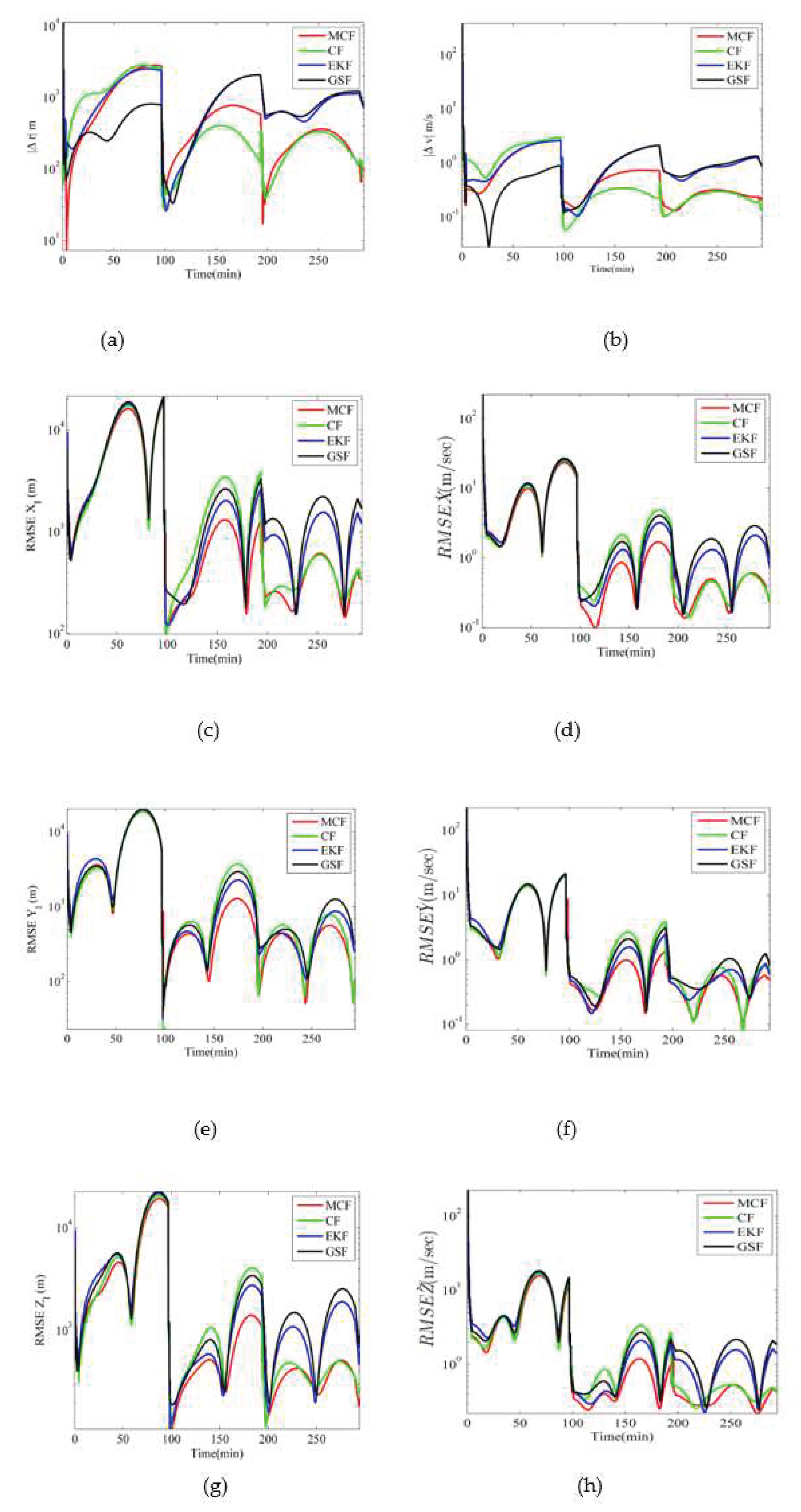
Now one extends the filtering performance for later orbital period i.e., once there are no observations available. Figure 2 depicts time history of IE and instantaneous RMSE (Equation (47)) over 3 orbital periods. The measurements (0.033 Hz) are only available for 4 min once the satellite is in viewing position from the radar site. These simulations are obtained from processing 50 Monte Carlo runs for each filter. The performance of CF and MCF are very close when compared for IE criteria, however, one may observe distinct improvement in RMSE results by MCF over other filtering methods.

5.3. MCF for Onboard Satellite Navigation Using GPS
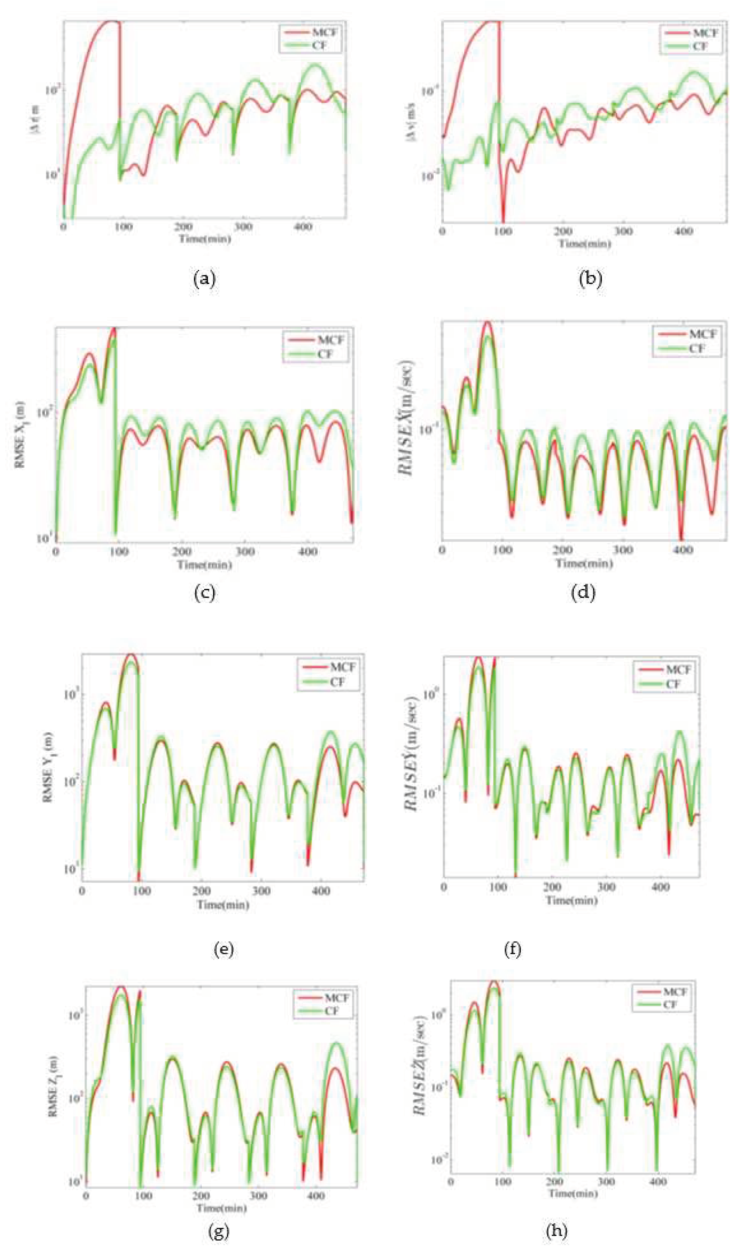
LEO small satellites are equipped with a GPS receiver such as SGR-05P of Surrey Satellite Technology (SSTL), whose position and velocity accuracy are 10 m and 0.15 m/s, respectively [48]. Due to limited power resource onboard small satellites, use of GPS for OD should be done carefully to conserve the power and enhance satellite’s mission lifetime. Now we compare MCF with CF for OD of an in-orbit satellite whose position and velocity are available after 95 min (~ 1 orbital period). The time history of IE and RMSE are shown in Figure 3.
Figure 3. Comparison of CF with MCF for position/velocity errors in ECI coordinates (shown in log scale) when measurement availability is once per orbital period (a to h).
Preprints 71134 g003
Figure 3 shows improvements achieved using MCF over CF. Convergence to lower errors is obtained by MCF in merely over 5 orbital periods. Therefore, by employing MCF one could increase mission lifetime of a satellite along with better OD. The error curves have also been produced by averaging using 50 Monte Carlo runs.

6. Conclusion

In this paper we have developed an improved nonlinear filter based on GCSM model approximation of Bayes’ aposteriori PDF for space object state estimation using radar measurements. Comparative analysis of our filter with other methods for tracking of space debris shows improvement/comparable performance under highly uncertain initial conditions and availability of sparse and no measurement data. MCF can also be used in other astrophysical computations such as motion and position of celestial bodies and satellites.

Funding

This research was funded by National University of Sciences and Technology, Pakistan.

Acknowledgments

I deeply acknowledge guidance and kindness of my PhD Supervisor P.L. Palmer (Late) who has left for hereafter on 24, November 2016.

Appendix A

A.1 Integral of product of two gaussian densities p g ( i ) and p g ( j ) :
e x p [ 1 / 2 2 π P ( i ) + P ( j ) × x μ i T P 1 i x μ i + x μ j T P 1 ( j ) x μ ( j ) ] d x
The bove integral can be re-expressed as [32]:
e x p [ K ( i ) ] 2 π d 2 P ( i ) + P ( j ) e x p 1 2 e ( i ) d ( i ) T Ω 1 e ( i ) d ( i ) d e ( i )
where,
K ( i ) = 1 2 z ( i ) T P 1 ( j ) Ω P 1 ( j ) P 1 ( j ) z ( i ) e ( i ) = x μ ( i ) z ( i ) = μ ( j ) μ ( i ) d ( i ) = Ω P 1 ( j ) z ( i ) Ω = P 1 ( i ) + P 1 ( j ) 1
A.2 Gaussian based expectation integrals can be expressed as [32]:
I 0 = e x p 1 2 x r b r T Ω r s 1 x s b s d x = 2 π d 2 Ω i j 1 / 2
I 1 = e x p 1 2 x r b r T Ω r s 1 x s b s x i b i d x = 0
I 2 = e x p 1 2 x r b r T Ω r s 1 x s b s x i b i x j b j d x = 2 π d 2 Ω i j 1 / 2 Ω i j
I 3 = e x p 1 2 x r b r T Ω r s 1 x s b s x i b i x j b j x k b k d x = 0
I 4 = e x p 1 2 x r b r T Ω r s 1 x s b s x i b i x j b j x k b k x l b l d x = 2 π d 2 Ω i j 1 / 2 Ω i j Ω k l + Ω i k Ω j l + Ω i l Ω j k
where, Ω i j 1 / 2 is determinant of Ω A.3 The components of matrix
M c (Equation (32)):
m c i j = 1 Δ t 2 e x p [ K ( j ) ] 2 π d 2 P ( i ) + P ( j ) + e x p [ K ( j ) ] P ( i ) + P ( j ) Ω i j 1 / 2 V ( j ) + e x p [ K ( i ) ] P ( i ) + P ( j ) Ω i j 1 / 2 V ( i )
where, the term for jth component are shown below:
K ( j ) = 1 2 z ( j ) T P 1 ( i ) Ω P 1 ( i ) P 1 ( i ) z ( j ) e j = x μ j z j = μ i μ j d j = Ω P 1 i z j Ω = P 1 i + P 1 j 1 V j = 1 2 P a b c 3 j η a j E b c j η a j = P a r 1 j d r j G a b j = Ω a e P e b 1 j Q a b j = P a e 1 j G e b j E b c ( j ) = Q a b ( j ) P a b 1 ( j ) + 1 3 η a ( j ) η b ( j )
For K ( i ) and V ( i ) replace “j” by “i” in Equation (56).
For i = j:
m c i i = 1 Δ t 2 1 2 π d 2 2 P ( i )
A.4 The components of matrix N c (Equation (32)) are expressed as:
n c i j = 1 Δ t p g c s ( i ) p g c s j T μ ( j ) μ ˙ ( j ) + T r p g c s j T P ( j ) P ˙ ( j ) + p g c s ( j ) P a b c ( 3 ) ( j ) P ˙ a b c ( 3 ) ( j ) 1 Δ t p g c s ( j ) + p g c s j T x f t , x + p g c s ( j ) T r f t , x x 1 2 T r Q 2 p g c s ( j ) x x T d x
We shall utilize tensor notations to solve the above integral analytically. Each of the above term inside the square bracket of integrand can be treated separately:
n c i j 1 = 1 Δ t + p g c s ( i ) p g c s j T μ j μ ˙ j d x
Substituting Equation (25) and taking expectation of the function inside bracket (Equation (59)) and making use of results given in Equation (48) to Equation (54) we obtain following:
n c i j 1 = 1 Δ t Ω i j 1 / 2 μ ˙ a ( j ) P ( i ) + P ( j ) { e x p [ K ( j ) ] η a ( j ) + P l m n 3 ( j ) 3 ! Q l m ( j ) Q n a ( j ) 3 + η l ( j ) η m ( j ) η n ( j ) η a ( j ) + Q l m ( j ) η n ( j ) η a ( j ) 3 + Q l a ( j ) η m ( j ) η n ( j ) 3 P m n 1 ( j ) Q l a ( j ) 3 P m n 1 ( j ) η l ( j ) η a ( j ) 3 P l a 1 ( j ) Q m n ( j ) 3 P l a 1 ( j ) η m ( j ) η n ( j ) 3 + P l a 1 ( j ) P m n 1 ( j ) [ 3 ] + e x p [ K ( i ) ] P l m n 3 ( i ) 3 ! Q l m ( i ) Q n a ( i j ) 3 + η l ( i ) η m ( i ) η n ( i ) ζ a ( j i ) + Q l m ( i ) η n ( i ) ζ a ( j i ) 3 + Q n a ( i j ) η l ( i ) η m ( i ) 3 P m n 1 ( i ) Q l a ( i j ) 3 P m n 1 ( i ) η l ( i ) ζ a ( j i ) 3 }
where, double superscript variables are:
Q n a ( i j ) P 1 i Ω P 1 j ζ a ( j i ) = P a u 1 ( j ) d u ( i ) z u ( i ) η a ( j i ) = P a u 1 ( j ) d u ( i )
Other variables used in above expression are like the Equation (55). Now we solve the second integrand of Equation (58) as:
n c i j 2 = 1 Δ t + p g c s ( i ) T r p g c s j T P ( j ) P ˙ ( j ) d x
By substituting Equation (26) in above equation the solution can be expressed as:
n c i j 2 = 1 Δ t Ω i j 1 / 2 P ˙ m l ( j ) P ( i ) + P ( j ) { e x p K ( j ) ( 1 2 Q l m ( j ) + η l ( j ) η m ( j ) P l m 1 ( j ) P a b c 3 ( j ) 3 ! [ 1 2 ( η l j Q m a j 3 P b c 1 j + η l j η m j η a j P b c 1 j + η l j Q m b j 3 P a c 1 j + η l j η m j η b j P a c 1 j + η l j Q m c j 3 P a b 1 j + η l j η m j η c j P a b 1 j + ( η a j Q b c j 3 ) P l m 1 ( j ) + η a ( j ) η b ( j ) η c ( j ) P l m 1 ( j ) ) 1 2 P l m 1 j ( P a b 1 j η c j 3 ) + η m j Q b c j 3 P a l 1 j + η m j η b j η c j P a l 1 j + η a j Q m c j 3 P b l 1 j + η a j η m j η c j P b l 1 j + η a j Q m b j 3 P c l 1 j + η a j η b j η m j P c l 1 j P a l 1 j P b c 1 j 3 η m j ( P b l 1 j P m c 1 j η a j 3 ) ] ) e x p K ( i ) P a b c 3 ( i ) 3 ! ( 1 2 ( η a i P b c 1 i [ 3 ] ) Q l m j + ( η a i P b c 1 i 3 ) ζ l j i ζ m j i + ( ( P a b 1 i Q m c i j 3 ) ζ l ( j i ) + P a b 1 i Q l c j i 3 ζ m j i + P l m 1 j ( η a i Q b c i 3 + η a i η b i η c i η a i P b c 1 i 3 ) ) }
where,
Q m c ( j i ) P 1 j Ω P 1 i
Now we solve the third integrand inside square bracket of Equation (58). The integrand can be written as:
n c i j 3 = 1 Δ t + p g c s ( i ) p g c s ( j ) P a b c ( 3 ) ( j ) P ˙ a b c ( 3 ) ( j ) d x
Substituting Equation (29) and using the results of Equation (48) to Equation (49), we perform expectations of above integral with respect p g c s ( i ) . The solution can be expressed as:
n c i j 3 = 1 Δ t Ω i j 1 / 2 e x p K ( j ) 3 ! P ( i ) + P ( j ) P ˙ a b c ( 3 ) ( j ) η a ( j ) E b c ( j ) [ 3 ]
See the Equation (55) for solution of fourth integrand of Equation (58) as these are identical:
n c i j 4 = 1 Δ t 2 + p g c s ( i ) p g c s ( j ) d x
Now we solve for 5th integrand of Equation (58):
n c i j 5 = 1 Δ t + p g c s ( i ) p g c s j T x f t , x d x
The solution of above integral can be simplified by expanding the nonlinear function up to second order in Taylor series and substituting Equation (27) in Equation (66). The solution can be written as:
n c i j 5 = 1 Δ t Ω i j 1 / 2 P ( i ) + P ( j ) [ e x p K ( j ) ( P a u 1 ( j ) d u j f a t , μ j + F a w j ( Ω u w + d u j d w j ) + A a w f j ( d u j Ω w f + d w j Ω u f + d f j Ω u w + d u j d w j d f j P l m n 3 ( j ) 3 ! ( f a t , μ j ( Q l m ( j ) Q n a ( j ) 3 + η l ( j ) η m ( j ) η n ( j ) η a ( j ) + Q l m ( j ) η n ( j ) η a ( j ) 3 + Q l a ( j ) η m ( j ) η n ( j ) 3 P m n 1 ( j ) Q l a ( j ) 3 P m n 1 ( j ) η l ( j ) η a ( j ) 3 P l a 1 ( j ) Q m n ( j ) + P l a 1 ( j ) η m ( j ) η n ( j ) 3 ) ( P l a 1 j η m j L n a j + η n j L m a j + ξ a j Q m n j + η m j η n j ξ a j ) 3 + f a t , μ j + F a w j d w j + A a w f j Ω w f + d w j d f j P l a 1 ( j ) P m n 1 ( j ) [ 3 ] ) ) ) + e x p K ( i ) P l m n 3 ( i ) 3 ! ( f a t , μ j ( P l m 1 ( i ) Q a n ( i j ) 3 + η l ( i ) ζ a ( j i ) P m n 1 ( i ) 3 ) + L a a ( j ) η l ( i ) P m n 1 ( i ) + Q a l ( j i ) P m n 1 ( i ) ξ a ( j i ) + ζ a ( j i ) L a l ( i j ) P m n 1 ( i ) + η l ( i ) P m n 1 ( i ) ξ a ( j i ) ζ a ( j i ) [ 3 ] ) ]
where, the new variables defined in above equation are:
F a w j = f a ( t , x ) x w x = μ ( j ) ,         A a w f j = 1 2 2 f a ( t , x ) x w x f x = μ ( j ) L ( j ) = P ( j ) Ω F T ( j ) , L ( i j ) = P ( i ) Ω F T ( j ) ξ a ( j ) = F a w j d w ( j ) ,         ξ a ( j i ) = F a w j d w ( i ) z w ( i )
Sixth integrand of Equation (58) is zero for OD problem considered in this paper:
n c i j 6 = 1 Δ t + p g c s ( i ) p g c s ( j ) T r f t , x x d x = 0
Seventh integrand of Equation (58) can be written as:
n c i j 7 = 1 2 Δ t + p g c s ( i ) 1 2 T r Q 2 p g c s ( j ) x x T d x
By substituting Equation (28) in Equation (69), the solution of this integral can be written as:
n c i j 7 = 1 2 Δ t Ω i j 1 / 2 Q m l P ( i ) + P ( j ) [ e x p K ( j ) ( Q l m ( j ) + η l ( j ) η m ( j ) P l m 1 ( j ) P a b c 3 ( j ) 3 ! ( ( η l ( j ) Q m a ( j ) 3 ) P b c 1 ( j ) + ( η l ( j ) Q m b ( j ) 3 ) P a c 1 ( j ) + ( η l ( j ) Q m c ( j ) 3 ) P a b 1 ( j ) + ( η a ( j ) Q b c ( j ) 3 ) P l m 1 ( j ) + η l ( j ) η m ( j ) ( η a ( j ) P b c 1 ( j ) 3 ) + η a ( j ) η b ( j ) η c ( j ) P l m 1 ( j ) P l m 1 ( j ) ( η a ( j ) P b c 1 ( j ) 3 ) P a l 1 ( j ) P b m 1 ( j ) η c ( j ) 6 ) ) e x p K ( i ) P a b c 3 ( i ) 3 ! ( ( η a i P b c 1 i [ 3 ] ) Q l m j + ( η a i P b c 1 i 3 ) ζ l j i ζ m j i + ( P a b 1 i Q m c i j 3 ) ζ l ( j i ) + P a b 1 i Q l c i j 3 ζ m j i + P l m 1 j ( η a i Q b c i 3 + η a i η b i η c i η a i P b c 1 i 3 ) ) ]
Now for i=j the component of matrix N c are expressed as:
n c i i = 1 Δ t p g c s ( i ) p g c s i T μ ( i ) μ ˙ ( i ) + T r p g c s i T P ( i ) P ˙ ( i ) + p g c s ( i ) P a b c ( 3 ) ( i ) P ˙ a b c ( 3 ) ( i ) 1 Δ t p g c s ( i ) + p g c s i T x f t , x + p g c s ( i ) T r f t , x x 1 2 T r Q 2 p g c s ( i ) x x T d x
We shall utilize tensor notations to solve the above integral analytically. Each of the above term inside the square bracket of integrand can be treated separately.
n c i i 1 = 1 Δ t + p g c s ( i ) p g c s i T μ i μ ˙ i d x
Substituting Equation (25) and taking expectations of the function inside square bracket (Equation (72)) and making use of results provided in Equation (48) to Equation (54), we obtain following:
n c i i 1 = 1 Δ t P ( i ) 1 / 2 μ ˙ a ( i ) 2 ( d / 2 ) 2 P ( i ) P l m n 3 ( i ) 3 ! 2 P l m ( i ) Q a n ( i ) 3 + P l a ( i ) Q m n ( i ) 3 P l a ( i ) P m n ( i ) 3
Now we solve the second integrand of Equation (71) as:
n c i i 2 = 1 Δ t + p g c s ( i ) T r p g c s i T P ( i ) P ˙ ( i ) d x
By substituting Equation (26) in above Equation (73) the solution can be expressed as:
n c i i 2 = 1 Δ t P ( i ) 1 / 2 P ˙ m l ( i ) 2 ( d / 2 ) 2 P ( i ) 1 2 Q l m ( i ) P l m 1 ( i )
Now we solve the third integrand inside square bracket of Equation (71). Substituting Equation (29) and using the results of Equation (48) and Equation (49), we perform expectation of the integral with respect to p g c s ( i ) . The solution can be expressed as:
n c i i 3 = 1 Δ t + p g c s ( i ) p g c s ( i ) P a b c ( 3 ) ( i ) P ˙ a b c ( 3 ) ( i ) d x = 0
The furth term inside the square bracket of Equation (71) can be expressed as:
n c i i 4 = 1 Δ t 2 + p g c s i p g c s i d x = 1 Δ t 2 P ( i ) 1 / 2 2 d 2 2 P ( i )
Now we solve for 5th integrand of Equation (71) as:
n c i i 5 = 1 Δ t + p g c s ( i ) p g c s i T x f t , x d x
The solution of the above integral can be simplified by expanding the nonlinear function up to second order in Taylor series and substituting Equation (27) in Equation (77). The solution can be written as:
n c i i 5 = 1 Δ t P ( i ) 1 / 2 2 d 2 2 P ( i ) P a u 1 ( i ) F a w i P u w 1 ( i ) + P l m n 3 ( i ) 3 ! f a t , μ i P l m ( i ) Q a n ( i ) 3 + P n a ( i ) Q l m ( i ) 3 f a t , μ i + A a w f i P w f 1 ( i ) P l a 1 ( i ) P m n 1 ( i ) [ 3 ]
Sixth integrand n c i i 6 = 0 , therefore, we solve for seventh integrand of Equation (71):
n c i i 7 = 1 Δ t + p g c s ( i ) 1 2 T r Q 2 p g c s ( i ) x x T d x
By substituting Equation (28) in Equation (79), the solution of the integral can be written as:
n c i i 7 = 1 2 Δ t P ( i ) 1 / 2 Q m l 2 d 2 2 P ( i ) Q l m ( i ) P l m 1 ( i )
Note: To find solutions of integrals in Appendix A, fourth and higher order moments and their multiplicative terms involving differentials are neglected.

References

  1. Montenbruck, O., Gill, E., “Satellite Orbits Models, Methods and Applications,” Published by Springer, 2005.
  2. Bar-Shalom,Y., Li,X,R., Kirubarajan,T., “Estimation with Application to Tracking and Navigation,” Wiley-Interscience Publication 2001.
  3. Kalman, R,E., “A New Approach to Linear Filtering and Prediction Problems,” Transaction of the AMSE Journal of Basic Engineering, 82 (D-Series): pages: 35-45 1960.
  4. Hicks, J.D., “Performance Comparison of an Extended Kalman Filter and an Iterated Extended Kalman Filter for Orbit Determination of Space Debris with Poor Apriori Information and Intermittent Observations” MS Thesis Auburn University, Dec 2012.
  5. Kerr, T.H., “Streamlining Measurement Iteration for EKF Target Tracking”, IEEE Transaction on Aerospace and Electronic Systems, Vol.27, No.2, Mar 1991.
  6. Coelho, M, d, F., et.al., “An Improved Extended Kalman Filter for Radar Tracking of Satellite Trajectories”, MDPI Designs, 2021,5,54. [CrossRef]
  7. Gordon, N., Salmond, D., Ewing, C., “Bayesian State Estimation for Tracking and Guidance using the Bootstrap Filter,” Journal of Guidance Control and Dynamics, Vol. 18, No. 6, pages. 1434-1443, Nov-Dec 1995.
  8. Lee, D.J., “Nonlinear Bayesian Filtering with Applications to Estimation and Navigation,” PhD Dissertation, Texas A&M University May 2005.
  9. Rawat. T.K., and Parthasarathy., “Satellite Tracking using a Second-Order Stochastic Nonlinear Filter”, HAIT Journal of Science and Engineering B, 2007 Holon Institute of Technology.
  10. Mehra, R,K., “A Comparison of Several Nonlinear Filters for Re-entry Vehicle Tracking”, IEEE Transaction on Automatic Control, AC-16, 4 Aug 1971, 307-319.
  11. DeMars, K.J., Bishop, R.H., Jah, M.K., “Antropy-Based Approach for Uncertainty Propagation of Nonlinear Dynamical System,” Journal of Guidance Control and Dynamics, Vol.36, No.4, Jul-Aug 2013.
  12. Alspach, D, L., Sorenson, H, W., “Nonlinear Bayesian Estimation using Gaussian Sum Approximation,” IEEE Transaction on Automatic Control, Vol. AC-17, No.4, Aug 1972.
  13. Anderson, B, D, O., Moore, J, B., “Optimal Filtering,” Prentice-Hall Information & System Science Series, 1979.
  14. Terejanu. G., Singla. P., et.al., “Uncertainty Propagation for Nonlinear Dynamic Systems Using Gaussian Mixture Model”, Journal of Guidance Control Dynamics, Vol.31, No.6, pages. 1622-1633, Nov-Dec 2008.
  15. Horwood, J.T., Poore, A.B., “Adaptive Gaussian Sum Filters for Space Surveillance,” IEEE Transactions on Automatic Control Vol.56, No.8, Aug 2011.
  16. Psiaki, M.L., “Gaussian Mixture Kalman Filter for Orbit Determination Using Angle-Only Data,” Journal of Guidance Control and Dynamics, Engineering Notes 2017.
  17. Terejanu, G., Singla, P., Singh, T., and Scott, P.D., “A Novel Gaussian Sum Filter Method for Accurate Solution to Nonlinear Filtering Problem”, IEEE 11th International Conference on Information Fusion, 2008.
  18. Merwe, R.V.D., “Sigma-Point Kalman Filters for Probabilistic Inference in Dynamic State-Space Models,” PhD Dissertation OGI School of Science & Engineering at Oregon Health & Science University, Apr 2004.
  19. Julier, S, J., and Uhlmann, J, K., “A New Extension for Kalman Filter to Nonlinear Systems,” In The Proceedings of AeroSense: The 11th International Symposium on Aerospace/Defense Sensing, Simulation and Controls, Orlando, FL, USA, 1997.
  20. Merwe, R.V.D., Wan, E.A., “Efficient Derivative-Free Kalman Filters for Online Learning”, European Symposium on Artificial Neural Networks, ISBN 2-930307-01-3, pp. 205-210, Burges (Belgium), Apr 2001.
  21. Zhou, W., Hou, J. “A New Adaptive Robust Unscented Kalman Filter for Improving the Accuracy of Target Tracking,” IEEE Access, date of publication 10 Jun 2019, D.O.I: 10.1109/Access.2019.2921794.
  22. Grewal. M.S., Weill. L.R., Andrews. A.P., “Global Positioning System Inertial Navigation and integration”, Wiley-Interscience Publication, 2007.
  23. Zhao, Y., “Cubature+Extended Hybrid Kalman Filtering Method and its Application in PPP/IMU Tightly-Coupled Navigation Systems,” IEEE Sensors Journals D.O.I: 10.1109/JSEN.2015.2469105, IEEE Sensors Journal, 2015.
  24. Pesonen.H., Piche.R., “Cubature-based Kalman Filters for Positioning,” 7th Workshop on Positioning, Navigation and Commuincation WPNC 2010.
  25. Doucet, A., Godsill, S., and Andrieu, C., “On Sequential Monte Carlo Sampling Methods for Bayesian Filtering,” Statistical Computing Vol. 10, No.3, pp. 197-208, 2000.
  26. Kotecha, J, H., Djuric, P, M., “Gaussian Particle Filtering,” IEEE Transactions on Signal Processing, Vol. 51, No. 10, pages. 2592-2601, Oct 2003.
  27. Kotecha, J, H., Djuric, P, M., “Gaussian Sum Particle Filtering for Dynamic State Space Models,” Proceedings of ICASSP-2001, Salt Lake City, Utah, May 2001.
  28. Wang, F., Zhang, J., Lin, B., and Li, X., “Two Stage Particle Filter for Nonlinear Bayesian Estimation” IEEE Access-Special Section on Multimedia Analysis for Internet of Things (IoT) D.O.I: 10.1109/ACCESS.2018.2808922, Date of Publication: Feb 23, 2018.
  29. http://mathworld.wolfram.com/HermitePolynomial.html [Viewed on: 24 Oct 2019].
  30. Charlier, C,V,L., “Uber Dir Darstelling Willkurlicher Funktionen,” Ark.Mat Astr.och Fys.2 No.20 1-35, 1906.
  31. McCullagh, P., “Tensor Methods in Statistics,” Publisher Chapman and Hall, 1987.
  32. Culver, C, O., “Optimal Estimation for Nonlinear Stochastic Systems,” PhD Dissertation Massachusetts Institute of Technology, Mar 13, 1969.
  33. Challa, S., Bar-Shalom, Y., Krishnamurthy, V., “Nonlinear Filtering using Gauss-Hermite Quadrature and Generalized Edgeworth Series”, Proceedings of the American Control Conference, Jun 1999.
  34. Challa, S., Bar-Shalom, Y., Krishnamurty, V., “Nonlinear Filtering via Generalized Edgeworth Series and Gauss-Hermite Quadrature,” IEEE Transaction on Signal Processing, Vol.48, No.6, Jun 2000.
  35. Gilani, S., “Nonlinear Bayesian Filtering Based on Mixture of Orthogonal Expansions,” PhD Dissertation Surrey Space Centre Mar 2012.
  36. Gilani, S., Palmer, P., “Nonlinear Bayesian Estimation Based on Mixture of Gram Charlier Series,” IEEE Aerospace Conference, Big Sky, Montana, USA, Mar 2012.
  37. Maybeck, P., “Stochastic Models, Estimation, and Control Vol. 1,” Academic Press London 1979.
  38. Risken, H., “The Fokker-Planck Equation Methods of Solutions and Applications,” Second Edition, Springer 1996.
  39. Daum, F., “Nonlinear Filters: Beyond the Kalman Filter,” IEEE Aerospace & Electronics Magazine Vol. 20, No. 8, Aug 2005.
  40. Muscolino, G., Ricciardi, G., Vasta, M., “Stationary and Non-Stationary Probability Density Function for Nonlinear Oscillators”, International Journal of Nonlinear Mechanics, Vol.32, No.6, pp 1051-1064, 1997.
  41. Van Hulle, M, M., “Edgeworth-Expanded Gaussian Mixture Density Modeling,” Journal of Neural Computation, Vol. 17, No. 8, Pages. 1706-1714, Aug 2005.
  42. http://www.mathworks.co.uk/ [Viewed on 27 Oct 2019].
  43. Dempster. A.P., Liard. N.M., and Rubin. D.B., “Maximum Likelihood for Incomplete Data via EM Algorithm,” Journal of Royal Statistical Society B, 39, 1-38.
  44. Redner. R.A., and Walker. H.F., “Mixture Densities, Maximum Likelihood and the EM algorithm”, SIAM Rev., 26, 195-239.
  45. https://github.com/SaeedKeshavarzi/ReBEL (Acccessed on 27 Apr 2019).
  46. Mehrholz, D., Leushacke, L., “Detecting, Tracking and Imaging Space Debris” European Space Agency Bulliten 109, Feb 2002.
  47. Vallado, D, A., “Fundamentals of Astrodynamics and Applications (Second Edition),” The Space Technology Library, Published by Microcosm Press and Kluwer Academic Publisher 2004.
  48. Ebinuma, T., Unwin, E., Underwood, M and Imre., C, “A miniaturized GPS receiver for space application”, IFAC Automatic control in Aerospace, 2004.
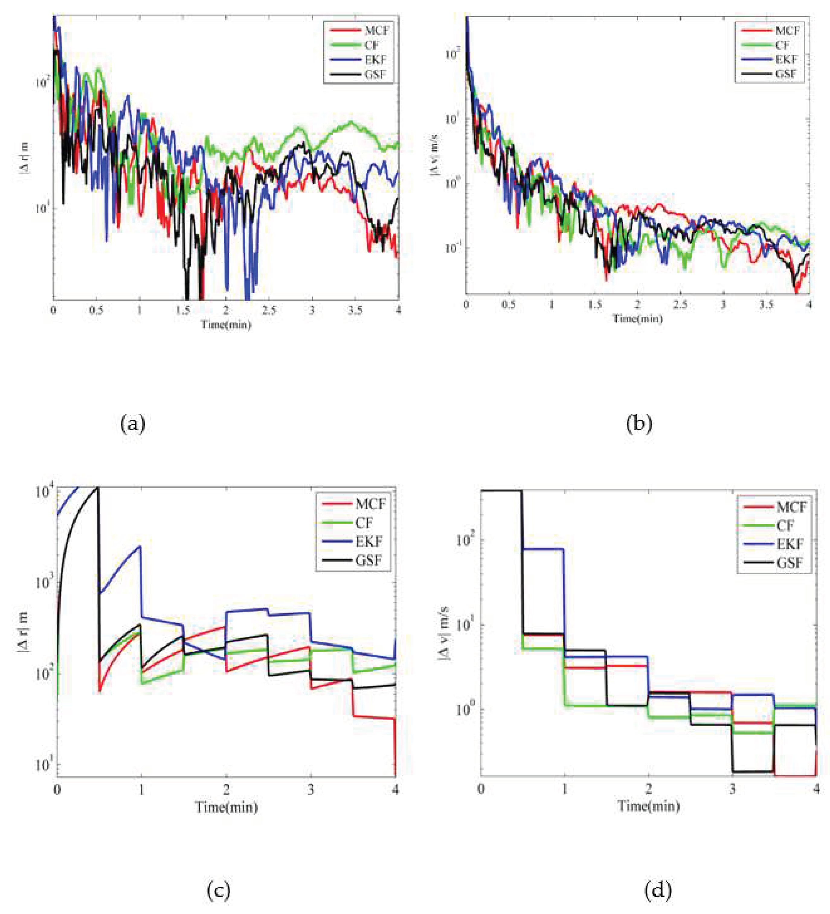
Figure 1. Comparison of filters with MCF for absolute position/velocity errors in ECI coordinates (shown in log scale) when measurement availability is 1 Hz (a & b) and 0.033 Hz (c & d).
Preprints 71134 g001
Figure 2. Comparison of filters with MCF for absolute position/velocity errors in ECI coordinates (shown in log scale) when measurement availability is 0.03 Hz during which the space debris appears on the sky for 4 min only (a to h).
Preprints 71134 g002
Table 1. MCF Algorithm.
Steps
1. Initial estimates/ higher order and noise statistics:
x ^ 0 + , P 0 + , P 0 + ( 3 ) , p W = N 0 , G Q G T
2. Perform Expectation Maximization (EM) to obtain GCSM from step.1.
3. Compute time update for states for g = 1 G
  • x ^ i ( k ) ( g ) = t k 1 t k d x ^ i g ( t ) d t = f i ( g ) x ^ , t + A i e f ( g ) x ^ , t P e f ( g ) d t
  • P i j ( k ) ( g ) = t k 1 t k d P i j ( g ) t d t = 2 F i e ( g ) x ^ , t P j e ( g ) + A i e f ( g ) x ^ , t P j e f 3 ( g ) s + V i j d t
  • P i j l ( k ) 3 ( g ) = t k 1 t k d P i j l 3 ( g ) t d t = 3 F i e ( g ) x ^ , t P j l e 3 ( g ) + A i e f g x ^ , t ( P j e g P l f g + P j f g P l e g ) s d t
where, V i j = individual components of diffusion matrix of SDE ( G Q G T )
4. Compute time update of GCSM weights, α k | k 1
5. Compute measurement update for g = 1 G
v k g = y k h x ^ k g , Λ k g = H k T g R 1 H k g , Ω k g = P k 1 g + Λ k g 1
d k g = Ω k g H k T g R 1 v k g , η k g = P k 1 g d k g , G k g = Ω k g P k 1 g , Q k g = P k 1 g G k g , E k g = Q k g P k 1 g + 1 3 η k g η k T g ,  
O k ( g ) = Q k ( g ) P k 1 ( g ) + η k ( g ) η k T ( g )
6. Compute tensors (time subscript “k” is removed from notations for clarity)
V ( g ) = 1 2 P a b c 3 ( g ) η a ( g ) E b c ( g ) , K ( g ) = 1 ( 1 + V ( g ) ) , ϕ i ( g ) = 1 2 K ( g ) P a b c 3 ( g ) G i a ( g ) O b c ( g )
φ i j g = K g P a b c g 3 η a g G i b g G j c g , N i j l g = K g P a b c 3 g G i a g G j b g G l c g
x ^ i + ( g ) = x ^ i ( g ) + d i ( g ) + ϕ i ( g ) , P i j + ( g ) = Ω i j g + φ i j ( g ) ϕ i ( g ) ϕ j ( g )
P i j l + 3 ( g ) = N i j l ( g ) ϕ i ( g ) φ j l ( g ) ϕ j ( g ) φ i l ( g ) ϕ l ( g ) φ i j ( g ) + 2 ϕ i ( g ) ϕ j ( g ) ϕ l ( g )
7. Compute weight updates:
α k ( g ) = α k 1 ( g ) D k 1 ( g ) g = 1 G α k 1 ( g ) D k 1 ( g )
8. Residual Resampling (optional step):
G E = 1 g = 1 G α k ( g ) 2
where, G E < G T is prescribed threshold criteria.
9. Compute inference: Conditional mean state estimates x ^ k + estimates and Covariance P k + :
x ^ k + = g = 1 G α k ( g ) x ^ k + ( g ) , P k + = g = 1 G α k ( g ) P k + ( g ) + x ^ k + ( g ) x ^ k + x ^ k + ( g ) x ^ k + T
Table 2. RMSE in ECI Coordinates for Filters with Measurement Availability of 0.033 Hz.
Filter Position RMSE (m) Velocity RMSE (m/s)
X Y Z X ˙ Y ˙ Z ˙
Extended Kalman Filter 2319 2392 2335 80 81 80
Culver Filter 1340 1328 1402 79 79 78
Mixture Culver Filter 1268 1423 1307 79 79 79
Gaussian Sum Filter 1298 1390 1316 79 79 79
Disclaimer/Publisher’s Note: The statements, opinions and data contained in all publications are solely those of the individual author(s) and contributor(s) and not of MDPI and/or the editor(s). MDPI and/or the editor(s) disclaim responsibility for any injury to people or property resulting from any ideas, methods, instructions or products referred to in the content.
Copyright: This open access article is published under a Creative Commons CC BY 4.0 license, which permit the free download, distribution, and reuse, provided that the author and preprint are cited in any reuse.
Prerpints.org logo

Preprints.org is a free preprint server supported by MDPI in Basel, Switzerland.

Subscribe

© 2024 MDPI (Basel, Switzerland) unless otherwise stated