Thermomechanical Peridynamic Modeling for Ductile Fracture

In this paper, we propose a modeling method based on peridynamics for ductile fracture at high temperatures. A thermoelastic coupling model combining peridynamics and classical continuum mechanics is used to limit the peridynamics calculations to the failure region of a given structure, thereby reducing computational costs. Then, a plastic constitutive model of peridynamic bonds is developed to capture the ductile-fracture process of the structure. Furthermore, an iterative algorithm for ductile-fracture calculation is presented. Finally, several numerical examples are shown. Particularly, the fracture processes of a superalloy structure under 800℃ and 900℃ environments are simulated and compared with experimental results. Our comparisons show that the crack modes captured by the proposed model are similar to experimental observations, which verifies the validity of the proposed model.

Keywords:

Subject: Engineering - Mechanical Engineering

1. Introduction

Many ductile materials, such as superalloys, are subjected to high temperatures for long periods, resulting in irreversible plastic deformation and even ductile fracture. Although researchers have conducted a number of numerical studies on the failure of ductile materials [1,2,3], the methods proposed are not suitable for predicting the process of crack initiation and propagation. A reason for this is that the constitutive models used and the corresponding numerical simulations were based on classical continuum mechanics (CCM). When CCM is used for fracture simulations, one inevitably encounters the singularity problem posed by discontinuities. To avoid the difficulties repeatedly encountered by CCM, a nonlocal solid mechanics theory called peridynamics (PD) was proposed by Silling in 2000 [4]. In recent years, the advantages of metal fracture modeling and numerical simulation based on PD are gradually becoming apparent [5,6].

PD assumes that there still are interactions between non-contact material points separated by a finite distance, and describes the mechanical behaviors of materials by solving integral equations of nonlocal effects in space, avoiding the singularity that occurs when CCM faces the fracture problem [7,8]. Therefore, PD models are suitable for simulating the fracture process and do not require complex crack propagation criteria [9].

However, nonlocal integration greatly increases calculation costs, and traditional traction boundary conditions cannot be applied directly in PD models. An effective way to solve this problem is to couple PD with CCM [10,11,12,13,14]. Lubineau et al. proposed a Morphing method to couple PD with CCM based on the principle of energy density balance [15], Azdoud et al. used this method to study quasi-static fracture problems [16]. Han et al. further developed a new model of coupling damage mechanics with PD through the Morphing method and used it to simulate the entire failure process of structures from elastic deformation and damage to complete fracture [17].

PD can be used to simulate not only the behavior of linear elastic materials but also the plastic deformation of materials. Macek and Silling proposed a perfectly elastoplastic bond constitutive model by permitting permanent deformation of individual bonds [18]. Zhan et al. proposed a rate-dependent plastic PD model to simulate the dynamic response of particle-reinforced metal matrix composites [19]. Madenci and Oterkus proposed an ordinary state-based PD model for plastic deformation based on von Mises yield criteria [20]. Liu et al. proposed an ordinary state-based PD model for nonlinear hardening plastic materials [21]. Although great progress has been made in the PD modeling of plastic materials, the above models did not take temperature into account. Both thermal and plastic deformation should be considered in the simulation of the plastic fracture of certain materials, such as superalloys.

In this paper, a plastic bond constitutive model is developed based on a thermoelastic bond-based PD model to describe the deformation and fracture of superalloys at high temperatures. The Morphing method is used to establish a thermoelastic model coupling PD with CCM to limit the plastic PD model to the fracture region, thereby reducing the computational cost.

The remainder of this paper is organized as follows: Section 2 proposes a new bond-based PD constitutive model by considering plasticity and thermal expansion in bond deformation. Section 3 derives a thermoelastic coupling model between PD and CCM through the Morphing method. Then, in Section 4, we describe an iterative algorithm of plastic-fracture calculations. We present numerical results for the fracture process in a superalloy structure and compare them with experimental observations in Section 5. Finally, Section 6 concludes the paper.

2. Thermal Elastoplastic Bond-based Peridynamic Model

PD theory assumes that there is an interaction between non-contact material points separated by a finite distance. Therefore, in the reference configuration

Ω

of the object, the interaction between any point

x

and a point

x^{'}

in its neighborhood is described by the pairwise force function

f

, and the balance equation at point

x

can be written as

\int_{H_{δ} (x)} f (x^{'}, x) d V_{x^{'}} + b (x) = 0

(1)

where

b

is a prescribed body force density and

H_{δ} (x) \subset Ω

is a circular region with

x

as its center and

δ

as its radius (see Figure 1). Thus,

δ

is referred to as the horizon [4].

The pairwise force function

f

is defined as

f (x^{'}, x) = \hat{f} (x^{'}, x) - \hat{f} (x, x^{'})

(2)

where

\hat{f} (x^{'}, x)

is the partial interaction due to the action of point

x^{'}

over point

x

and, correspondingly,

\hat{f} (x, x^{'})

is the partial interaction due to the action of point

x

over point

x^{'}

. By introducing plastic deformation and thermal expansion into the bond deformation calculation, the partial interaction can be written as

\hat{f} (x^{'}, x) = \frac{1}{2} c (x, ξ) (η_{ξ} (x^{'}, x) - {\bar{η}}_{ξ} - a (x, ξ) \hat{T} (x, ξ)) e_{ξ}

(3)

where

ξ = x^{'} - x

is the relative position vector herein referred to as “bond",

η_{ξ} (x^{'}, x) = η (x^{'}, x) \cdot e_{ξ}

denotes the projection of the bond deformation at point

x

over the bond,

η (x^{'}, x) = u (x^{'}) - u (x)

, and

e_{ξ} = \frac{ξ}{|ξ|}

. In addition,

u

is the displacement and

e_{ξ}

is the unit direction vector of the bond. In Eq.(3),

a (x, ξ) \hat{T} (x, ξ)

represents the deformation of the bond due to thermal expansion [22], where

a (x, ξ)

is the coefficient of thermal expansion of the bond in the PD model. We define

\hat{T} (x, ξ)

as the effective temperature of the bond. In other words,

\hat{T}

is determined by

T (x)

and

T (x^{'})

, which are the temperature variations between the current temperatures and the reference temperatures of points

x

and

x^{'}

, respectively. Thus, we have

\hat{T} (x, ξ) = \hat{T} (x^{'}, - ξ)

(4)

Moreover,

{\bar{η}}_{ξ} = \bar{η} \cdot e_{ξ}

, where

\bar{η}

is the historical plastic elongation of the bond defined by:

\bar{η} (0) = 0, \dot{\bar{η}} = \{\begin{matrix} \dot{η} & if \frac{|ξ + η - \bar{η}| - | ξ |}{| ξ |} \geq s_{Y} \\ 0 & otherwise \end{matrix}

(5)

where

s_{Y}

is the yield stretch. It can be seen that, at the bond level, this material is elastic-perfectly plastic. However, for the entire structure, the material model has a strain hardening effect because not all bonds will yield at a certain moment or under deformation. It is worth noting that

s_{Y}

is an intrinsic parameter of the material, and its value is related to its engineering ultimate strength [18]. Moreover, the fracture behavior of materials can be described via bond failure [23]. It is assumed that the bond will break irreversibly if its stretch s exceeds the critical value

s_{C}

(generally,

s_{C} > s_{Y}

), where

s = \frac{|ξ + η| - | ξ |}{| ξ |}

After introducing a plastic elongation at the bond level, we then give an average measure of non-local plastic deformation at a point, which can be expressed as:

ϕ_{p} (x) = \frac{\int_{H_{δ} (x)} \bar{s} d V_{ξ}}{\int_{H_{δ} (x)} d V_{ξ}}

(6)

where

\bar{s} = \frac{| ξ + \bar{η} | - | ξ |}{| ξ |}

is the plastic stretch of a bond.

3. Thermoelastic Hybrid Peridynamics and Classical Continuum Mechanics (PD-CCM) Model

Hybrid PD-CCM models retain the advantages of PD in discontinuities and improve calculation efficiency [10,11,12,13,14]. In this section, we adopt the Morphing method [15] to establish a thermoelastic hybrid PD-CCM model.

3.1. Governing Equations

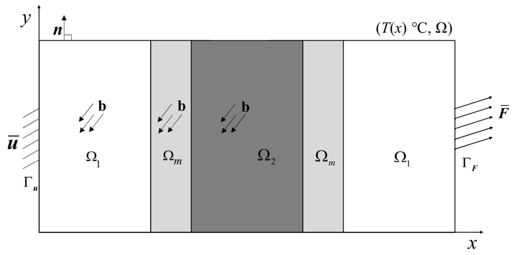
We divide the whole solution region into three non-overlapping subregions, i.e.,

Ω = Ω_{1} \cup Ω_{2} \cup Ω_{m}

, and

Ω_{1} \cap Ω_{2} = \emptyset

Ω_{1} \cap Ω_{m} = \emptyset

Ω_{2} \cap Ω_{m} = \emptyset

. The PD model is confined to subregion

Ω_{2}

, where plastic deformation and fracture may occur, and the CCM model is employed in subregions

Ω_{1}

to reduce computational costs. The two models transition through subregion

Ω_{m}

. As shown in Figure 2, the displacement boundary condition

\bar{u}

is applied to part

Γ_{u}

\partial Ω

, and the traction load

\bar{F}

is applied to part

Γ_{F}

\partial Ω

n

is a unit vector representing the outer normal, and the entire solution region

Ω

is affected by the body force

b

and the steady-state temperature field

T (x)

The Morphing method is based on a set of governing equations that are valid for any point in

Ω

, and it defines the material properties of the two models as functions that change with position [24]. The governing equations are as follows:

Kinematic admissibility and compatibility

$\begin{matrix} ε (x) & = \frac{1}{2} (\nabla u (x) + {(\nabla u)}^{T} (x)) & \forall x \in Ω ∖ Ω_{2} \end{matrix}$

(7)

$\begin{matrix} η_{ξ} (x^{'}, x) & = u_{ξ} (x^{'}) - u_{ξ} (x) & \forall x, x^{'} \in Ω ∖ Ω_{1} \end{matrix}$

(8)

$\begin{matrix} u (x) & = \bar{u} (x) & \forall x \in Γ_{u} \end{matrix}$

(9)
Static admissibility

$\begin{matrix} div σ (x) + \int_{H_{δ} (x)} f (x^{'}, x) d V_{x^{'}} & = - b (x) & \forall x \in Ω \end{matrix}$

(10)

$\begin{matrix} σ (x) \cdot n (x) & = \bar{F} & \forall x \in Γ_{F} \end{matrix}$

(11)
Constitutive equations

$\begin{matrix} σ (x) & = E (x) : ε (x) - β (x) T (x) & \forall x \in Ω ∖ Ω_{2} \\ f (x^{'}, x) & = \frac{1}{2} (c (x, ξ) + c (x^{'}, ξ)) (η_{ξ} (x^{'}, x) - {\bar{η}}_{ξ}) e_{ξ} \end{matrix}$

(12)

$\begin{matrix} - \frac{1}{2} (b (x, ξ) \hat{T} (x, ξ) + b (x^{'}, ξ) \hat{T} (x^{'}, - ξ)) e_{ξ} & \forall x \in Ω ∖ Ω_{1} \end{matrix}$

(13)

Here,

σ

and

ε

are the stress and strain tensors, respectively. In Eq.(12),

E (x)

is the stiffness tensor, and

β (x) = E (x) : α (x)

is the thermal modulus, where

α (x)

is the thermal expansion coefficient tensor.

For homogeneous materials, the PD micromodulus function

c (x, ξ)

and the thermal expansion coefficient function

a (x, ξ)

can be redefined as:

c (x, ξ) = w (x) c^{0} (| ξ |)

(14)

a (x, ξ) = v (x) a^{0} (| ξ |)

(15)

where

w (x)

and

v (x)

are the Morphing functions,

0 \leq w (x), v (x) \leq 1, \forall x \in Ω

c^{0} (| ξ |)

and

a^{0} (| ξ |)

are the PD micromodulus and thermal expansion coefficient, respectively. We define the PD thermal modulus as

b^{0} (| ξ |) = c^{0} (| ξ |) a^{0} (| ξ |)

. Then, the pairwise force function

f

can be rewritten as in Eq.(13), where

b (x, ξ) = w (x) v (x) b^{0} (| ξ |)

(16)

3.2. Stiffness/Thermal Modulus Constraint Equations

The overall governing equations of the hybrid model were given in Section 3.1. It can be seen that the functions

w (x)

v (x)

and

E (x)

β (x)

jointly guide the transition between the CCM and PD model.

w (x)

and

v (x)

are the functions that determine the division of the hybrid model, so how we define

E (x)

and

β (x)

is key to successfully couple both models together. In this subsection, we derive the constraint functions of

E (x)

and

β (x)

based on the point-by-point equivalency of energy density.

The plastic deformation is confined to the pure peridynamic region, that is,

{\bar{η}}_{ξ} \equiv 0

outside this region. Thus, the constitutive equation in Equation (13) can be simplified to an elastic version. Let us consider a subregion

Ω_{0} = {x \in Ω : H_{δ} (x) \subset Ω}

, such that we still have a complete integral region when the PD model is used near the boundary. We can derive the following equations according to previous work [24]. The following assertions hold true for any point

x \in Ω_{0}

If and only if $E (x) = E^{0}$ , $β (x) = β^{0}$ and $w (x^{'}), v (x^{'}) = 0$ , $\forall x^{'} \in H_{δ} (x)$ , the model is restricted to the pure CCM model at point $x$ . Then the elastic energy density at point $x$ can be written as

$W (x) = \frac{1}{2} ε (x) : E^{0} : ε (x) - ε (x) : β^{0} T (x) + W^{0} (T)$

(17)
If and only if $E (x) = 0$ , $β (x) = 0$ and $w (x^{'}), v (x^{'}) = 1$ , $\forall x^{'} \in H_{δ} (x)$ , the model is restricted to the pure PD model at point $x$ . Considering Equation (4), the elastic energy density at point $x$ can be written as

$W (x) = \frac{1}{4} \int_{H_{δ} (x)} c^{0} (| ξ |) η_{ξ}^{2} (x^{'}, x) d V_{x^{'}} - \frac{1}{2} \int_{H_{δ} (x)} b^{0} (| ξ |) \hat{T} (x, ξ) η_{ξ} (x^{'}, x) d V_{x^{'}} + W^{0} (T)$

(18)
If and only if $E (x) \neq 0$ , $β (x) \neq 0$ and $\exists x^{'} \in H_{δ} (x)$ such that $0 < w (x) < 1, 0 < v (x) \leq 1$ , the hybrid model must be used at point $x$ . Considering Equation (4), the elastic energy density at point $x$ can be written as

$\begin{matrix} W (x) = \frac{1}{2} ε (x) : E (x) : ε (x) + \frac{1}{4} \int_{H_{δ} (x)} c^{0} (| ξ |) \frac{w (x^{'}) + w (x)}{2} η_{ξ}^{2} (x^{'}, x) d V_{x^{'}} + W^{0} (T) \\ - ε (x) : β (x) T (x) - \frac{1}{2} \int_{H_{δ} (x)} b^{0} (| ξ |) \frac{w (x^{'}) v (x^{'}) + w (x) v (x)}{2} \hat{T} (x, ξ) η_{ξ} (x^{'}, x) d V_{x^{'}} \end{matrix}$

(19)

Remark:

W^{0} (T)

corresponds to the

T^{2}

term in the elastic energy density equations.

For homogeneous materials, the elastic energy density at any point should be independent of the definition of the Morphing functions

w (x)

and

v (x)

and only depend on the displacement and temperature field. This means that the elastic energy densities calculated at the same point with different expressions are equivalent to each other, and thus the corresponding terms of force and temperature must be equal. Therefore, the terms of Equation (17) are equal to the corresponding ones in Equation (18) respectively, i.e.,

\begin{matrix} \frac{1}{2} ε (x) : E^{0} : ε (x) & = \frac{1}{4} \int_{H_{δ} (x)} c^{0} (| ξ |) η_{ξ}^{2} (x^{'}, x) d V_{x^{'}} \end{matrix}

(20)

\begin{matrix} ε (x) : β^{0} T (x) & = \frac{1}{2} \int_{H_{δ} (x)} b^{0} (| ξ |) \hat{T} (x, ξ) η_{ξ} (x^{'}, x) d V_{x^{'}} \end{matrix}

(21)

Furthermore, we assumed that both temperature and elastic deformation in the small neighborhood of point

x

are uniform such that

ε (x^{'}) ≃ ε (x) = \bar{ε} and η_{ξ} (x^{'}, x) = \frac{ξ \cdot \bar{ε} \cdot ξ}{| ξ |}, \forall x^{'} \in H_{δ} (x)

(22)

\hat{T} (x, ξ) ≃ T (x) = \bar{T}, \forall x^{'} \in H_{δ} (x)

(23)

Thus, Equations (20) and (21) leads to:

\begin{matrix} E^{0} & = \frac{1}{2} \int_{H_{δ} (x)} c^{0} (| ξ |) \frac{ξ \otimes ξ \otimes ξ \otimes ξ}{{| ξ |}^{2}} d V x^{'} \end{matrix}

(24)

\begin{matrix} β^{0} & = \frac{1}{2} \int_{H_{δ} (x)} b^{0} (| ξ |) \frac{ξ \otimes ξ}{| ξ |} d V x^{'} \end{matrix}

(25)

Similarly, the terms of Equation (17) are equal to the corresponding ones in Equation (19), and by considering Equations (22)–(25) we get

\begin{matrix} E (x) & = E^{0} - \frac{1}{2} \int_{H_{δ} (x)} c^{0} (| ξ |) \frac{w (x^{'}) + w (x)}{2} \frac{ξ \otimes ξ \otimes ξ \otimes ξ}{{| ξ |}^{2}} d V x^{'} \end{matrix}

(26)

\begin{matrix} β (x) & = β^{0} - \frac{1}{2} \int_{H_{δ} (x)} b^{0} (| ξ |) \frac{w (x^{'}) v (x^{'}) + w (x) v (x)}{2} \frac{ξ \otimes ξ}{| ξ |} d V x^{'} \end{matrix}

(27)

In summary, the thermoelastic hybrid PD-CCM model is established by Equations (7)–(16), (26) and (27). The partitioning of the hybrid model is determined by the Morphing functions

w (x)

and

v (x)

, and the definitions of

w (x)

and

v (x)

are independent of each other.

4. Plastic-Fracture Calculations

In this paper, the constraint equations of the hybrid model are used to ensure that PD applies only in the critical region where plastic deformation and cracks may occur. The plastic bond constitutive equation defined in Equation (3) is used to perform iterative calculations.

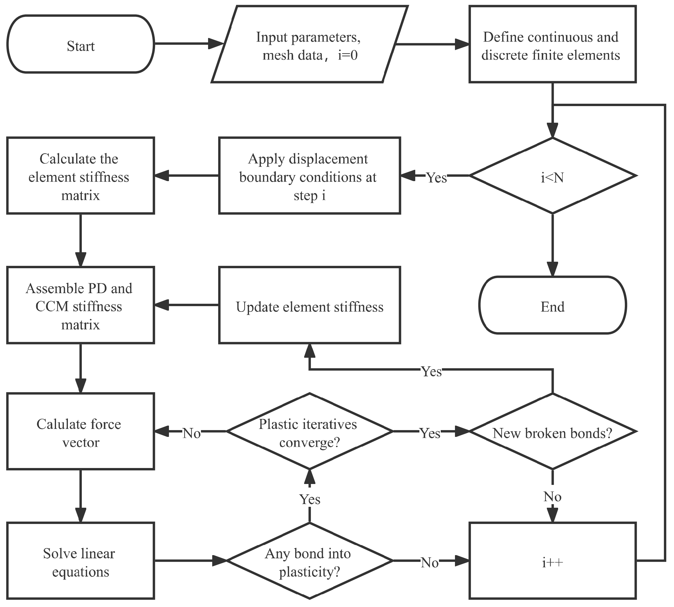
Figure 3 shows the flowchart of the implicit iterative algorithm used for plastic-fracture simulation. In this algorithm, the coupling zone and the CCM zone are discretized by continuous finite elements, whereas the pure PD zone is discretized by discrete finite elements [25]. Discrete elements allow cracks to grow freely along their boundaries. The boundary conditions are imposed gradually in N increments. In each incremental step, the elongation of each bond is calculated according to the displacement field obtained by solving the corresponding linear equations. If any bond yields, the residual plastic force needs to be calculated to update the force vector at the right side of the equations. This step is repeated until the iterative solution of the system of linear equations converges.

After the plastic iterative calculation converges, if any bonds break at the current step, it is necessary to update the stiffness matrix by removing the contribution of these bonds. Change in the stiffness matrix will inevitably alter the calculated displacement field, so it is necessary to recalculate the residual plastic force and solve the equations until the plastic iteration converges and no bonds break anymore at the current step. Afterwards, the step is incremented and calculations are repeated until the last load step is completed.

5. Numerical Examples

This section presents two numerical examples to validate the proposed model. The first is a two-dimensional simplified model of an actual experiment involving a GH4099 superalloy structure under high-temperature environments. We compare the simulated fracture modes and force-displacement curves with the experimental results to assess the ability of the proposed model for simulating the failure of ductile materials. The second numerical example involves a four-point bending beam under uniform and non-uniform temperature fields to investigate the effects of temperature field and plastic deformation on crack propagation.

5.1. Example 1: GH4099 Superalloy Structure

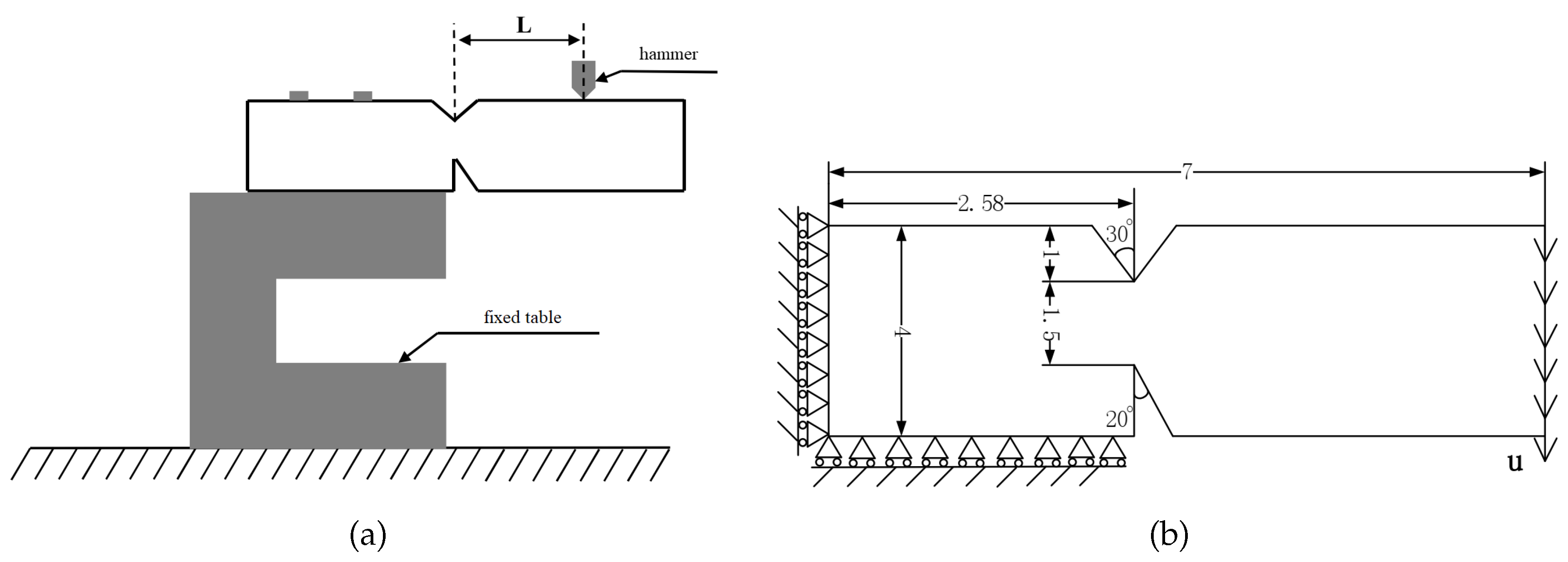
The geometry of the experimental GH4099 superalloy specimen is shown in Figure 4. As shown in Figure 4b, the top of the specimen is preset with a

60^{0}

angle V-shaped groove with a depth of 1mm, whereas the bottom is preset with a

20^{0}

angle weakening groove with a depth of 1.5mm. The experimental setup is shown in Figure 5a. The distance between the loading hammer and the weakening groove is

L = 24.5

mm, and the hammer loads slowly and vertically downwards, which can be considered as quasi-static loading. The focus of this simulation is on the crack mode. The cracking position of the structure is far away from the load application region, and its deformation is only related to the resultant force and moment of the load. According to the Saint--Venant principle, the specific distribution of the load only affects the stress distribution around the load application region. The error caused by this approximation is confined near the loading boundary. Therefore, considering the requirements of computational efficiency, we scaled the length dimension according to the equivalent of the resultant moment at the groove position. On the other hand, because the ratio of the width to the thickness of the experimental specimen is 10:1, we adopted the plane strain assumption to simplify the three-dimensional structure to a two-dimensional numerical specimen. The dimensions of the numerical specimen and the boundary conditions are shown in Figure 5b.

A grid of the geometric model is shown in Figure 6a. The model was discretized using four-node quadrilateral elements with a total of 2093 nodes and 2009 elements. The grid size was 0.1mm in the region delimited by

y \in [0, 4], x \in [1.2, 4]

and uniformly transitioned outside of this region from 0.1mm along the x direction to 0.4mm at the two boundaries. Figure 6b shows the value distribution of the Morphing function

w (x)

. From Equations (26) and (27), it can be seen that the model partitions are determined by the values of

w (x)

and

w (x) v (x)

. We preset

v (x) = 1

for the whole body

Ω

, that is, the model partition was only affected by the value distribution of

w (x)

. Thus, in Figure 6b, the red region corresponds to the pure PD model (

w (x) = 1

), the blue region corresponds to the pure CCM model (

w (x) = 0

), and the transition region is the coupled model (

0 < w (x) < 1

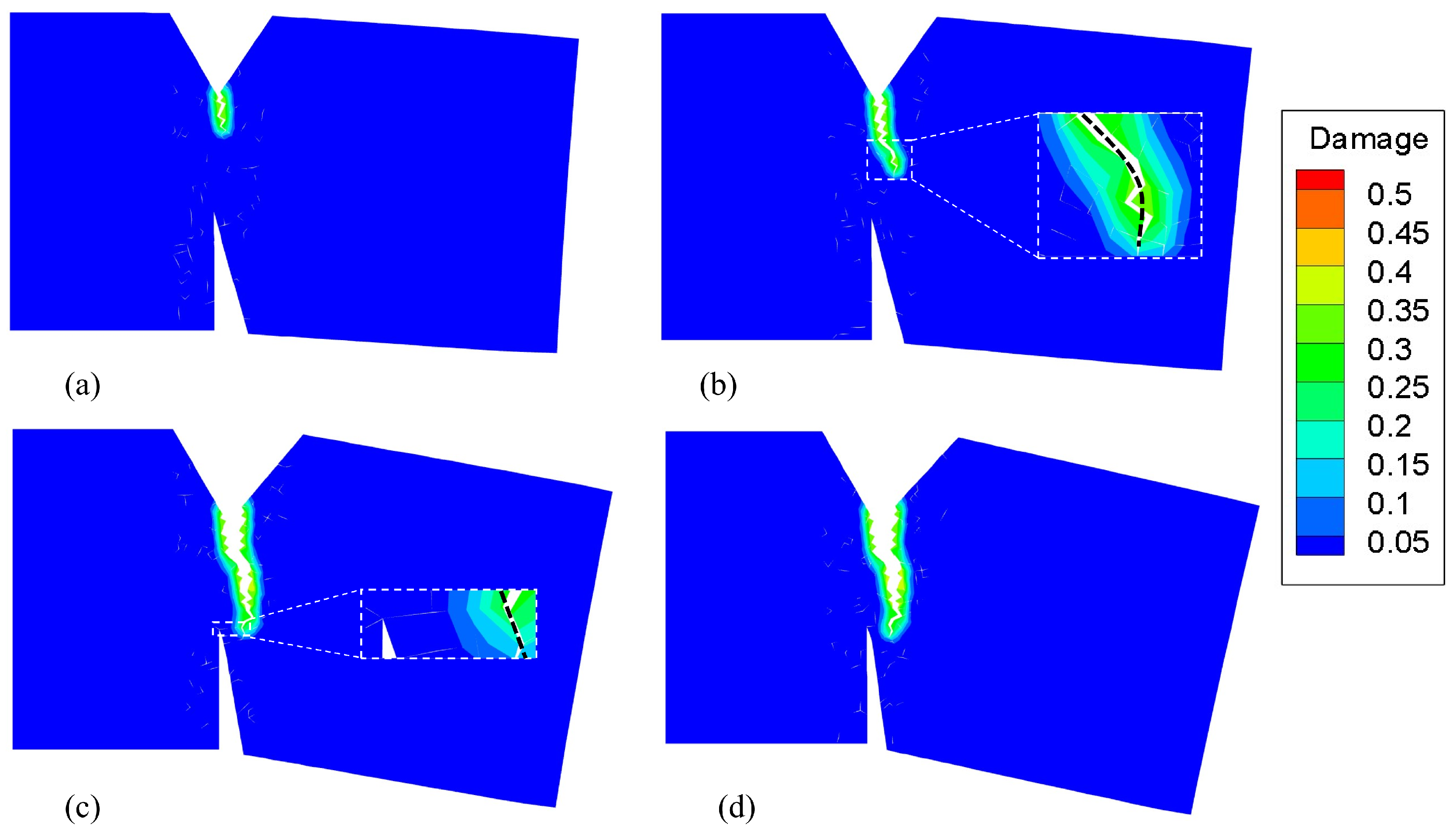
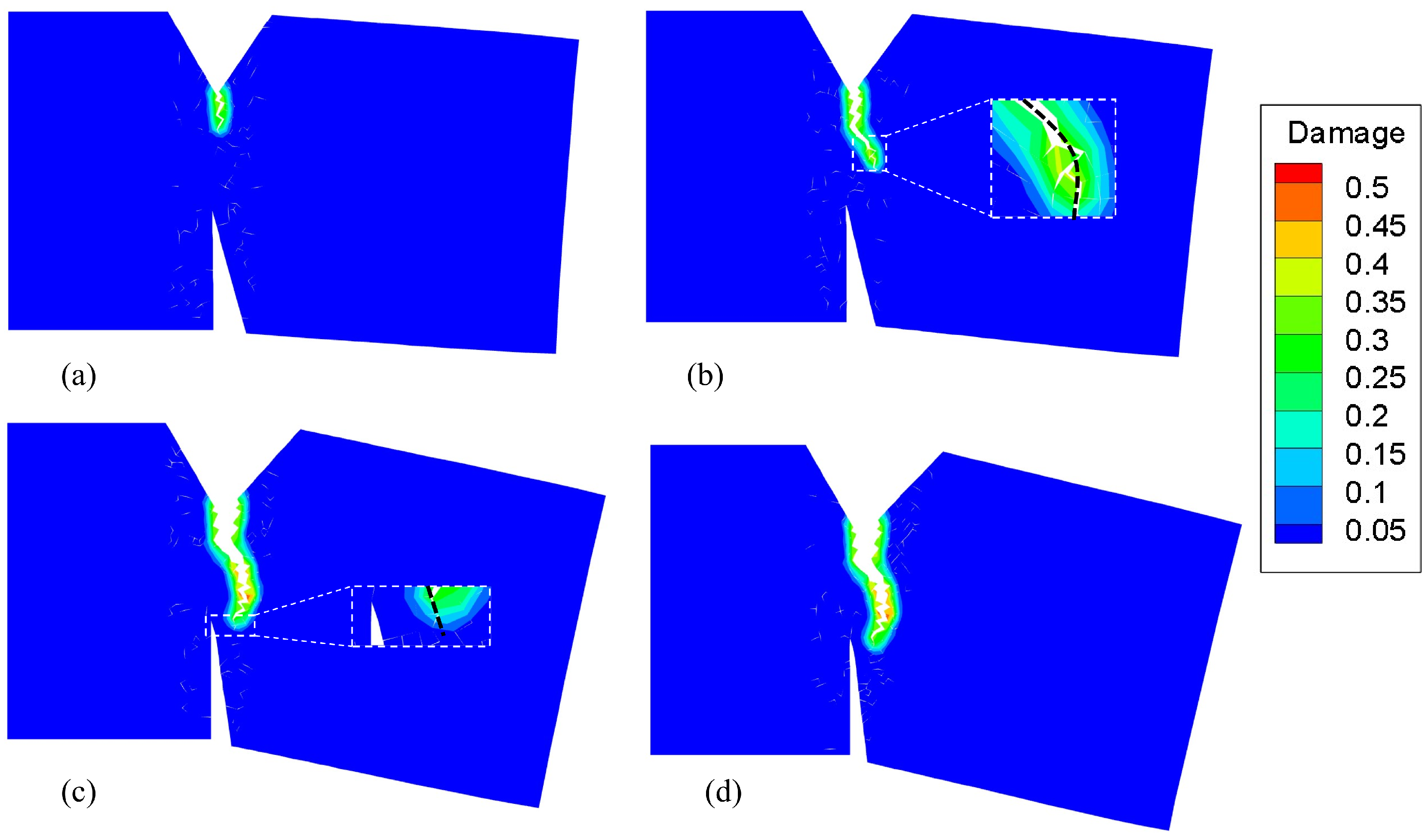
Because the bond-based PD model was used, Poisson’s ratio for plane strain problems was fixed at 1/4 [4,26]. The horizon

δ

of the PD model was set to 0.3mm and the displacement increment was

Δ \bar{u} = 0.018 mm

. At 800°C, the Young’s modulus of the GH4099 superalloy is 147GPa, and its thermal expansion coefficient is

15.1 \times 10^{- 6} / ° C

. The yield (

s_{Y}

) and critical (

s_{C}

) stretch were set to 0.04 and 0.1 respectively. Figure 7a shows the damage contour at the 15th loading step. Owing to the ductility of the superalloy material at 800°C, the initial crack propagation direction is affected by the V-groove at the top of the structure and has a certain angle with the vertical direction, which is different from that of a brittle fracture. As the loading progresses, the crack continues to propagate along the initial direction. By the 20th loading step (see Figure 7b), the crack starts to deflect toward the bottom weakening groove. By the 40th loading step (see Figure 7c), the crack has propagated to the vicinity of the tip of the weakening groove, then the crack propagation direction becomes parallel to the hypotenuse of the weakening groove. In this state, the structure is difficult to completely fracture. Thus, after the 50th loading step (see Figure 7d), the crack does not continue to grow as loading increases.

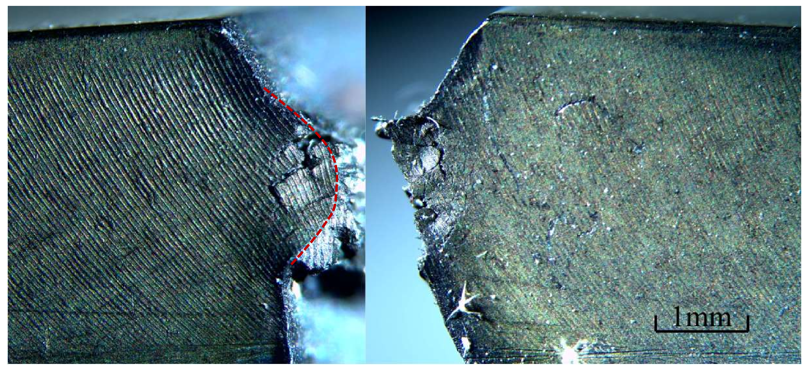
At 900°C, the Young’s modulus of the GH4099 superalloy is 121GPa and its thermal expansion coefficient is

15.3 \times 10^{- 6} / ° C

. The yield (

s_{Y}

) and critical (

s_{C}

) stretch were set to 0.04 and 0.12, respectively. The simulation results obtained under a 900°C environment are shown in Figure 8. The whole fracture process is similar to that at 800°C. The direction of crack propagation changes from the 16th step to the 24th step, as shown in Figure 8a,b. Afterwards, the crack propagates to the vicinity of the tip of the weakening groove and the path becomes parallel to the hypotenuse of the weakening groove by the 48th step. After the 54th loading step, the crack stops growing. However, the crack propagation direction deflects in a more pronounced way compared with the results obtained at 800°C. Figure 9 shows a photomicrograph of the GH4099 superalloy structure at 900°C. An arc-shaped crack path can be seen in the figure, which is consistent with the simulated crack path.

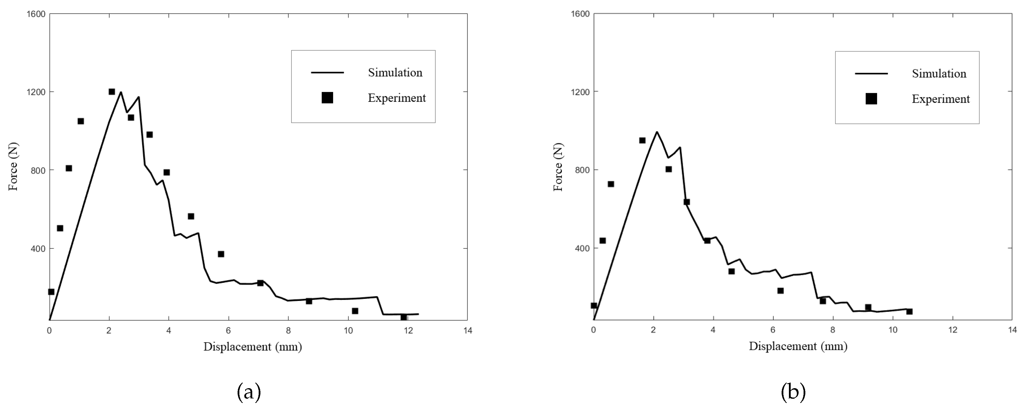
To further verify the effectiveness of the proposed model for simulating ductile fracture at high temperatures, the force-displacement curves obtained from the simulations and experiments at 800°C and 900°C were compared, and the results are shown in Figure 10. Unlike in brittle fractures, the force does not quickly decrease to zero after reaching the peak value. The simulation results were in good agreement with the experimental results. In both the simulations and experiments, it can be seen that, at the end of the curve, the force does not decrease with an increase of displacement but remains constant. This indicates that in the final stage of the failure process of superalloy structures, the structure does not further fracture as the loading progresses. This coincides with the simulated final crack mode. By comparing the force-displacement curves of 800°C and 900°C, we can see that the peak force at 900°C is significantly lower than that at 800°Cowing to the softening effect of the high-temperature environment on the alloy. Additionally, the displacements of both crack initiation and final break decrease, which shows that superalloy structures become more prone to failure as temperature rises.

5.2. Example 2: Four-point bending beam

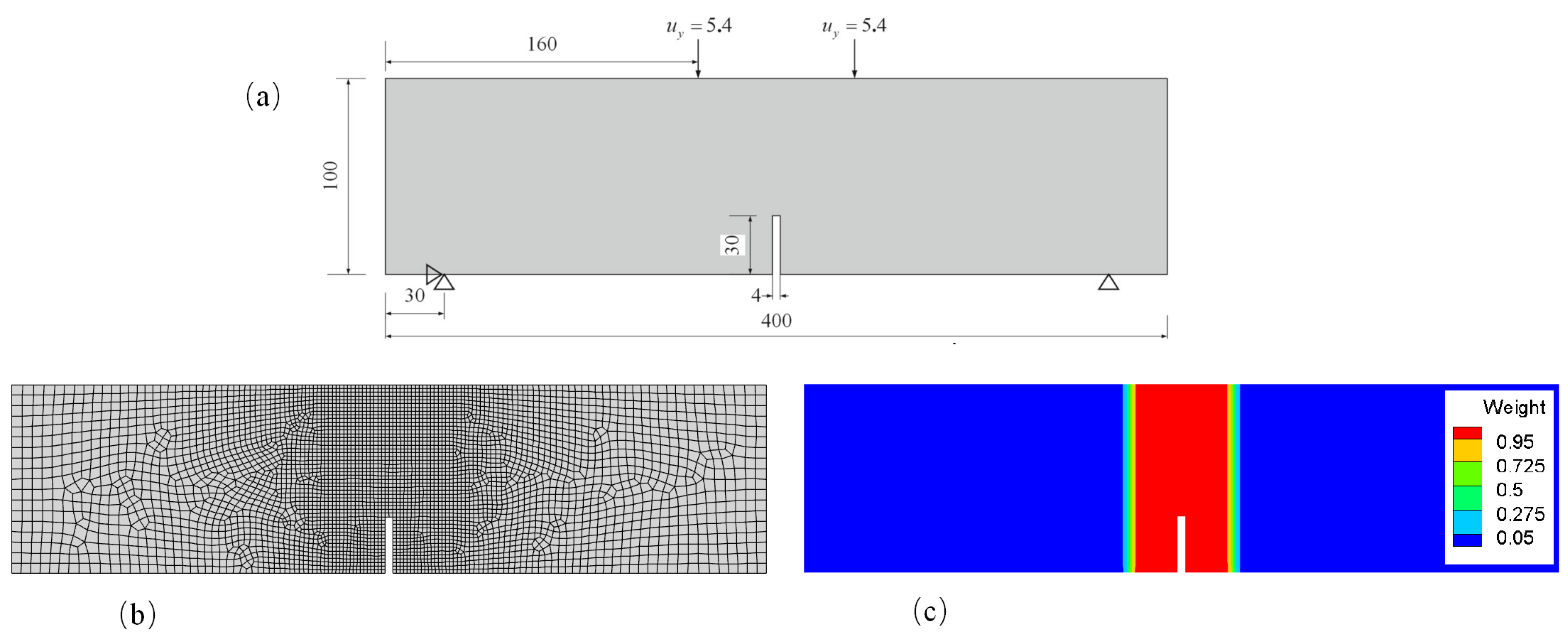
This example aims to illustrate the effect of the temperature field and plastic deformation on crack propagation paths. The geometry and boundary conditions for this numerical example are shown in Figure 11a. The grid of this example is shown in Figure 11b, and the grid size in the PD region was set to 2mm. Figure 11c shows the value of the morphing function

w (x)

, which indicates the scope of the different models. The fracture process of the four-point bending beam was simulated under two different temperature conditions, namely a uniform temperature field of 500°C (Figure 12a) and a non-uniform temperature field transitioning from 0°C to 1000°C (Figure 12b). This setting ensures that the specimen is always at 500°C in the vertical direction of the notch of the beam.

To consider the influence of plastic deformation and temperature on the crack path of the four-point bending beam, four numerical tests with the same Young’s modulus and thermal expansion coefficient were conducted. The parameter settings for the four numerical tests are listed in Table 1. For all numerical tests, the horizon

δ

was set to three times the grid size of the PD region. The example assumes a plane-stress condition, so Poisson’s ratio is fixed at 1/3.

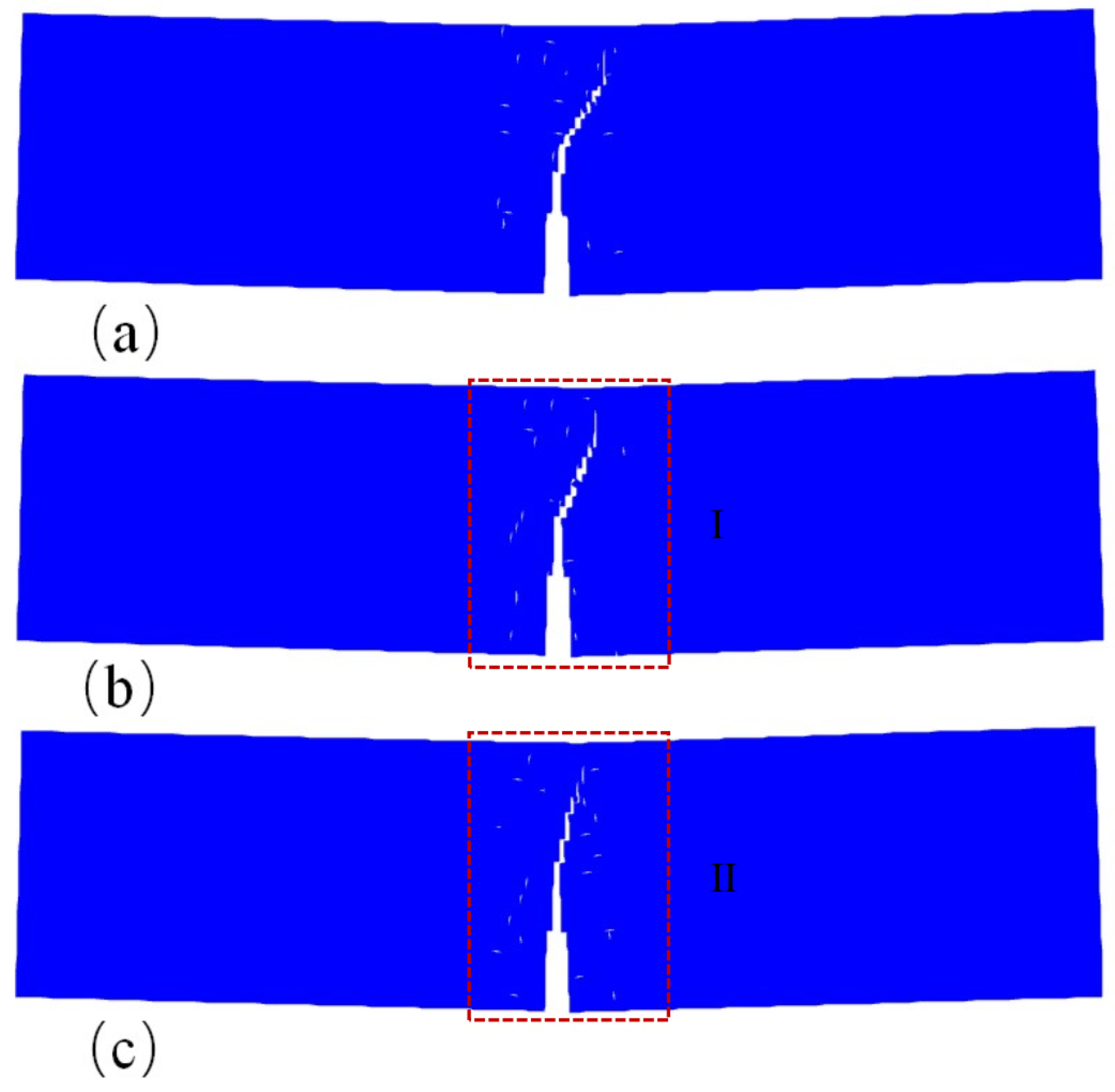
First, we compared the crack paths of the four-point bending beam under different temperature conditions. Figure 13 shows the final crack paths of cases 1 and 3. These two cases had the same parameter settings except for temperature, but nonetheless exhibited different crack modes. It can be seen that under the uniform temperature field (see Figure 13a), the crack propagates along the vertical direction of the notch of the beam, whereas it propagates along a different path under the non-uniform temperature field (see Figure 13b). This is because there is a transverse temperature gradient in the non-uniform temperature field, which leads to non-uniform thermal expansion at the left and right ends of the beam, resulting in the deflection of the crack.

In cases 2, 3, and 4, the numerical simulations are performed under the non-uniform temperature field, but plastic deformation was only allowed in cases 3 and 4. Thus, in case 2, a bond breaks immediately after its deformation reaches the elastic limit (which is considered a brittle fracture). In cases 3 and 4, an admissible plastic elongation of

\bar{s} = 0.005

and

\bar{s} = 0.01

is introduced after the deformation of a single bond reaches the elastic limit, respectively. The elastic limit of the bond was the same for these three cases. Figure 14 shows the final crack paths of the four-point bending beam for cases 2, 3 and 4. By comparing the crack paths of these three cases, it can be seen that the angle of the crack path in case 2 deviates the most from the vertical direction under the non-uniform temperature field(see Figure 14a). In addition, the deflection angle of the crack path decreases with the increase of the admissible plastic deformation of the bond.

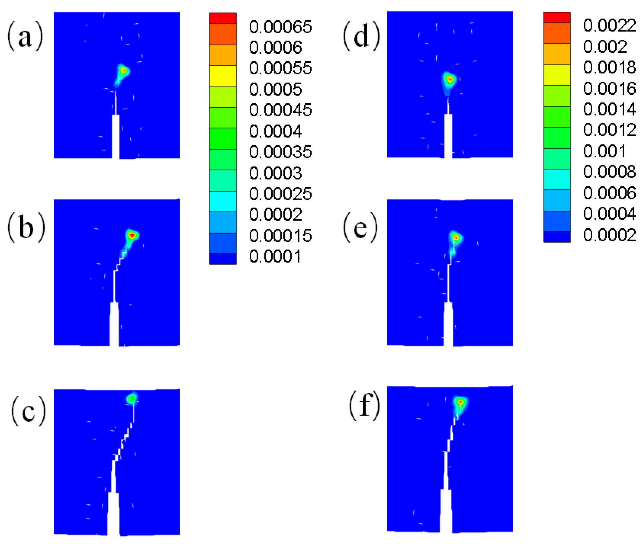
We also analyzed the plastic deformation zone of the crack tip during crack propagation in cases 3 and 4. In Figure 15, subfigures (a), (b) and (c) show the plastic deformation zones around the crack tip at the 10th, 15th and 25th loading steps, respectively, corresponding to region I in Figure 14. On the other hand, subfigures (d), (e), and (f) show the plastic deformation zones around the crack tip at the 10th, 15th and 25th loading steps, corresponding to region II in Figure 14. The color indicates the value of the non-local plastic deformation calculated by Equation (6). It can be seen that, compared with case 3, the crack tip in case 4 is accompanied by a greater nonlocal plastic deformation during the crack propagation. This greater nonlocal plastic deformation around the crack tip weakens the influence of the temperature gradient on the crack path. Therefore, in case 4, the angle at which the crack path deviates from the vertical direction is smaller than that in case 3.

6. Conclusion

We proposed a plastic-fracture PD model for fracture simulation in ductile materials that can accurately simulate plastic deformation and the fracture process under different temperature conditions. We simulated the plastic-fracture process of a GH4099 superalloy structure at 800°C and 900°C. The simulation results show that the proposed model predicts an arc-shaped crack path, which was observed in experiments. The simulated fracture modes and force–displacement curves were in good agreement with our experimental results, demonstrating the effectiveness of the proposed model for simulating ductile fracture at high temperatures. We also carried out numerical tests of a four-point bending beam under uniform and non-uniform temperature fields. The effects of temperature and plastic deformation on the crack path are discussed. The results show that the plastic deformation zone around the crack tip weakens the impact of temperature on the crack deflection.

Funding

This research was funded by the National Natural Science Foundation of China (12272082) and the National Key Laboratory of Shock Wave and Detonation Physics (JCKYS2021212003).

Institutional Review Board Statement

Not applicable.

Informed Consent Statement

Not applicable.

Data Availability Statement

Data sharing is not applicable to this article.

Conflicts of Interest

The authors declare no conflict of interest.

References

Li, Y.F.; Zeng, X.G.; Chen, H.Y. A Three-dimensional dynamic constitutive model and its finite element implementation for NiTi alloy based on irreversible thermodynamics. Acta Mechanica Solida Sinica 2019, 32, 356–366. [Google Scholar] [CrossRef]
Liang, W.; Hu, X.; Zheng, Y.; Deng, D. Determining inherent deformations of HSLA steel T-joint under structural constraint by means of thermal elastic plastic FEM. Thin-Walled Structures 2020, 147, 106568. [Google Scholar] [CrossRef]
Fan, Z.X.; Kruch, S. A comparison of different crystal plasticity finite-element models on the simulation of nickel alloys. Materials at High Temperatures 2020, 37, 328–339. [Google Scholar] [CrossRef]
Silling, S.A. Reformulation of elasticity theory for discontinuities and long-range forces. Journal of the Mechanics and Physics of Solids 2000, 48, 175–209. [Google Scholar] [CrossRef]
Wu, C.T.; Ren, B. A stabilized non-ordinary state-based peridynamics for the nonlocal ductile material failure analysis in metal machining process. Computer Methods in Applied Mechanics and Engineering 2015, 291, 197–215. [Google Scholar] [CrossRef]
Zhan, J.; Yao, X.; Han, F.; Zhang, X. A rate-dependent peridynamic model for predicting the dynamic response of particle reinforced metal matrix composites. Composite Structures 2021, 263, 113673. [Google Scholar] [CrossRef]
Askari, A.; Azdoud, Y.; Han, F.; Lubineau, G.; Silling, S. 12 - Peridynamics for analysis of failure in advanced composite materials. In Numerical Modelling of Failure in Advanced Composite Materials; Hallett, S.R., Camanho, P.P., Eds.; Woodhead Publishing, 2015; pp. 331–350. [Google Scholar]
Bobaru, F.; Foster, J.T.; Geubelle, P.H.; Silling, S.A. (Eds.) Handbook of Peridynamic Modeling; Advances in Applied Mathematics, Chapman and Hall/CRC, 2016. [Google Scholar]
Ha, Y.D.; Bobaru, F. Characteristics of dynamic brittle fracture captured with peridynamics. Engineering Fracture Mechanics 2011, 78, 1156–1168. [Google Scholar] [CrossRef]
Han, F.; Lubineau, G. Coupling of nonlocal and local continuum models by the Arlequin approach. International Journal for Numerical Methods in Engineering 2012, 89, 671–685. [Google Scholar] [CrossRef]
Agwai, A.; Guven, I.; Madenci, E. Damage prediction for electronic package drop test using finite element method and peridynamic theory. Electronic Components & Technology Conference, 2009.
Kilic, B.; Madenci, E. Coupling of peridynamic theory and the finite element method. Journal of mechanics of materials and structures 2010, 5, 707–733. [Google Scholar] [CrossRef]
Oterkus, E.; Madenci, E.; Weckner, O.; Silling, S.A.; Bogert, P.; Tessler, A. Combined finite element and peridynamic analyses for predicting failure in a stiffened composite curved panel with a central slot. Composite Structures 2012, 94, 839–850. [Google Scholar] [CrossRef]
Liu, W.Y.; Hong, J.W. A coupling approach of discretized peridynamics with finite element method. Computer Methods in Applied Mechanics and Engineering 2012, 245-246, 163–75. [Google Scholar] [CrossRef]
Lubineau, G.; Azdoud, Y.; Han, F.; Rey, C.; Askari, A. A morphing strategy to couple non-local to local continuum mechanics. Journal of the Mechanics and Physics of Solids 2012, 60, 1088–1102. [Google Scholar] [CrossRef]
Azdoud, Y.; Han, F.; Lubineau, G. The morphing method as a flexible tool for adaptive local/non-local simulation of static fracture. Computational Mechanics 2014, 54, 711–722. [Google Scholar] [CrossRef]
Han, F.; Lubineau, G.; Azdoud, Y. Adaptive coupling between damage mechanics and peridynamics: A route for objective simulation of material degradation up to complete failure. Journal of the Mechanics and Physics of Solids 2016, 94, 453–472. [Google Scholar] [CrossRef]
Macek, R.W.; Silling, S.A. Peridynamics via finite element analysis. Finite elements in analysis and design 2007, 43, 1169–1178. [Google Scholar] [CrossRef]
Zhan, J.M.; Yao, X.H.; Han, F.; Zhang, X.Q. A rate-dependent peridynamic model for predicting the dynamic response of particle reinforced metal matrix composites. Composite Structures 2021, 263, 113673. [Google Scholar] [CrossRef]
Madenci, E.; Oterkus, S. Ordinary state-based peridynamics for plastic deformation according to von Mises yield criteria with isotropic hardening. Journal of the Mechanics and Physics of Solids 2016, 86, 192–219. [Google Scholar] [CrossRef]
Liu, Z.M.; Bie, Y.H.; Cui, Z.Q.; Cui, X.Y. Ordinary state-based peridynamics for nonlinear hardening plastic materials’ deformation and its fracture process. Engineering Fracture Mechanics 2020, 223, 106782. [Google Scholar] [CrossRef]
Kilic, B.; Madenci, E. Peridynamic Theory for Thermomechanical Analysis. IEEE Transactions on Advanced Packaging 2010, 33, 97–105. [Google Scholar] [CrossRef]
Silling, S.A.; Askari, E. A meshfree method based on the peridynamic model of solid mechanics. Computers & Structures 2005, 83, 1526–1535. [Google Scholar]
Liu, Z.Y.; Liu, S.K.; Han, F.; Chu, L.S. The Morphing method to couple local and non-local thermomechanics. Computational Mechanics 2022, 1–18. [Google Scholar] [CrossRef]
Li, Z.B.; Han, F. The peridynamics-based finite element method (PeriFEM) with adaptive continuous/discrete element implementation for fracture simulation. Engineering Analysis with Boundary Elements 2023, 146, 56–65. [Google Scholar] [CrossRef]
Silling, S.A.; Lehoucq, R.B. Peridynamic Theory of Solid Mechanics. Advances in Applied Mechanics 2010, 44, 73–168. [Google Scholar]

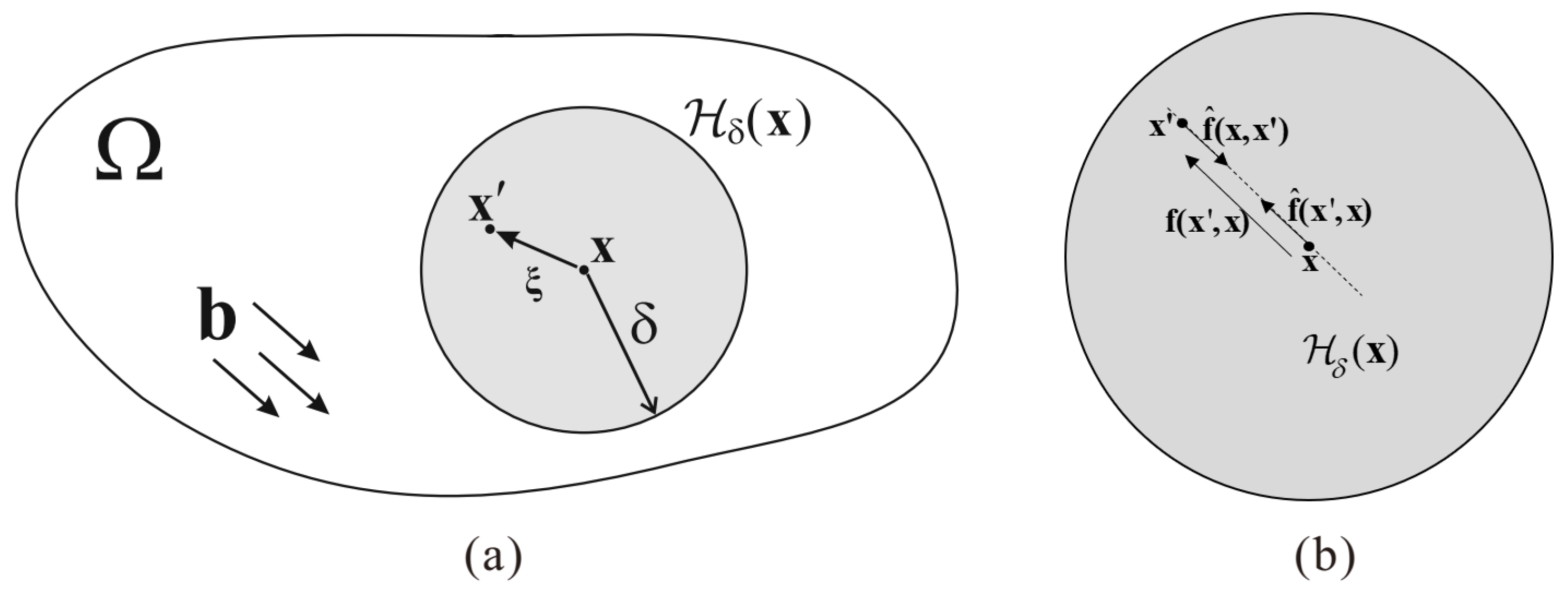
Figure 1. (a) Nonlocal continuum

Ω

and (b) partition of the interaction

f (x^{'}, x)

into partial interactions.

Figure 1. (a) Nonlocal continuum

Ω

and (b) partition of the interaction

f (x^{'}, x)

into partial interactions.

Figure 2. Region

Ω

consists of

Ω_{1}

Ω_{2}

and

Ω_{m}

Figure 2. Region

Ω

consists of

Ω_{1}

Ω_{2}

and

Ω_{m}

Figure 3. Flowchart of the iterative algorithm of the peridynamic plastic-fracture model.

Figure 4. (a) Schematic diagram of the experimental specimen geometry (unit: mm) and (b) groove details.

Figure 5. (a) Experimental setup and (b) simplified numerical model. (unit: mm)

Figure 6. (a) Grid and (b) value distribution of the Morphing function. (for interpretation of the references to color in this figure, the reader is referred to the web version of this paper).

Figure 7. Damage contour and crack propagation path of a superalloy structure at 800°Cat the (a) 15th step, (b) 20th step, (c) 40th step, and (d) 50th step. (for interpretation of the references to color in this figure, the reader is referred to the web version of this paper).

Figure 8. Damage contour and crack propagation path of a superalloy structure at 900°C at the (a) 16th step, (b) 24th step, (c) 48th step, and (d) 54th step. (for interpretation of the references to color in this figure caption, the reader is referred to the web version of this paper).

Figure 9. Experimental observations of the final fracture pattern at 900°C.

Figure 10. Simulated and experimental force-displacement curves at (a) 800°C and (b) 900°C.

Figure 11. Schematic diagram of the four-point bending beam: (a) geometry and boundary conditions, (b) grid and (c) value distribution of the Morphing function. (for interpretation of the references to color in this figure, the reader is referred to the web version of this paper).

Figure 12. Two different temperature conditions used for the numerical simulations of the four-point bending beam: (a) uniform temperature field, (b) non-uniform temperature field. (for interpretation of the references to color in this figure, the reader is referred to the web version of this paper).

Figure 13. Final crack paths of (a) case 1 and (b) case 3.

Figure 14. Crack paths for the three cases under a non-uniform temperature field: (a) case 2, (b) case 3, and (c) case 4.

Figure 15. Nonlocal plastic deformation contours. (a), (b), and (c) correspond to the 10th, 15th, and 25th loading steps for region I in Figure 14, respectively. (d), (e), and (f) correspond to the 10th, 15th, and 25th loading steps for region II in Figure 14, respectively. (For interpretation of the references to color in this figure caption, the reader is referred to the web version of this paper.)

Table 1. Material and numerical parameters.

Cases	Young’s modulus(GPa)	Coefficient of thermal expansion( $10^{- 6} / ° C$ )	$s_{Y}$	$s_{C}$	Temperature conditions	Increments
case 1	200	15.6	0.02	0.025	Figure 12a	30
case 2	200	15.6	∖	0.02	Figure 12b	30
case 3	200	15.6	0.02	0.025	Figure 12b	30
case 4	200	15.6	0.02	0.03	Figure 12b	30

Disclaimer/Publisher’s Note: The statements, opinions and data contained in all publications are solely those of the individual author(s) and contributor(s) and not of MDPI and/or the editor(s). MDPI and/or the editor(s) disclaim responsibility for any injury to people or property resulting from any ideas, methods, instructions or products referred to in the content.

© 2023 by the authors. Licensee MDPI, Basel, Switzerland. This article is an open access article distributed under the terms and conditions of the Creative Commons Attribution (CC BY) license (http://creativecommons.org/licenses/by/4.0/).

Copyright: This open access article is published under a Creative Commons CC BY 4.0 license, which permit the free download, distribution, and reuse, provided that the author and preprint are cited in any reuse.

MDPI Initiatives

Important Links

Choose an area of interest and we will send you notifications of new preprints at your preferred frequency.

Disclaimer

Thermomechanical Peridynamic Modeling for Ductile Fracture

Abstract

1. Introduction

2. Thermal Elastoplastic Bond-based Peridynamic Model

3. Thermoelastic Hybrid Peridynamics and Classical Continuum Mechanics (PD-CCM) Model

3.1. Governing Equations

3.2. Stiffness/Thermal Modulus Constraint Equations

4. Plastic-Fracture Calculations

5. Numerical Examples

5.1. Example 1: GH4099 Superalloy Structure

5.2. Example 2: Four-point bending beam

6. Conclusion

Funding

Institutional Review Board Statement

Informed Consent Statement

Data Availability Statement

Conflicts of Interest

References

MDPI Initiatives

Important Links

Subscribe