Submitted:
28 April 2023
Posted:
28 April 2023
You are already at the latest version
Abstract
Keywords:
1. INTRODUCTION
2. MATERIAL AND METHODS
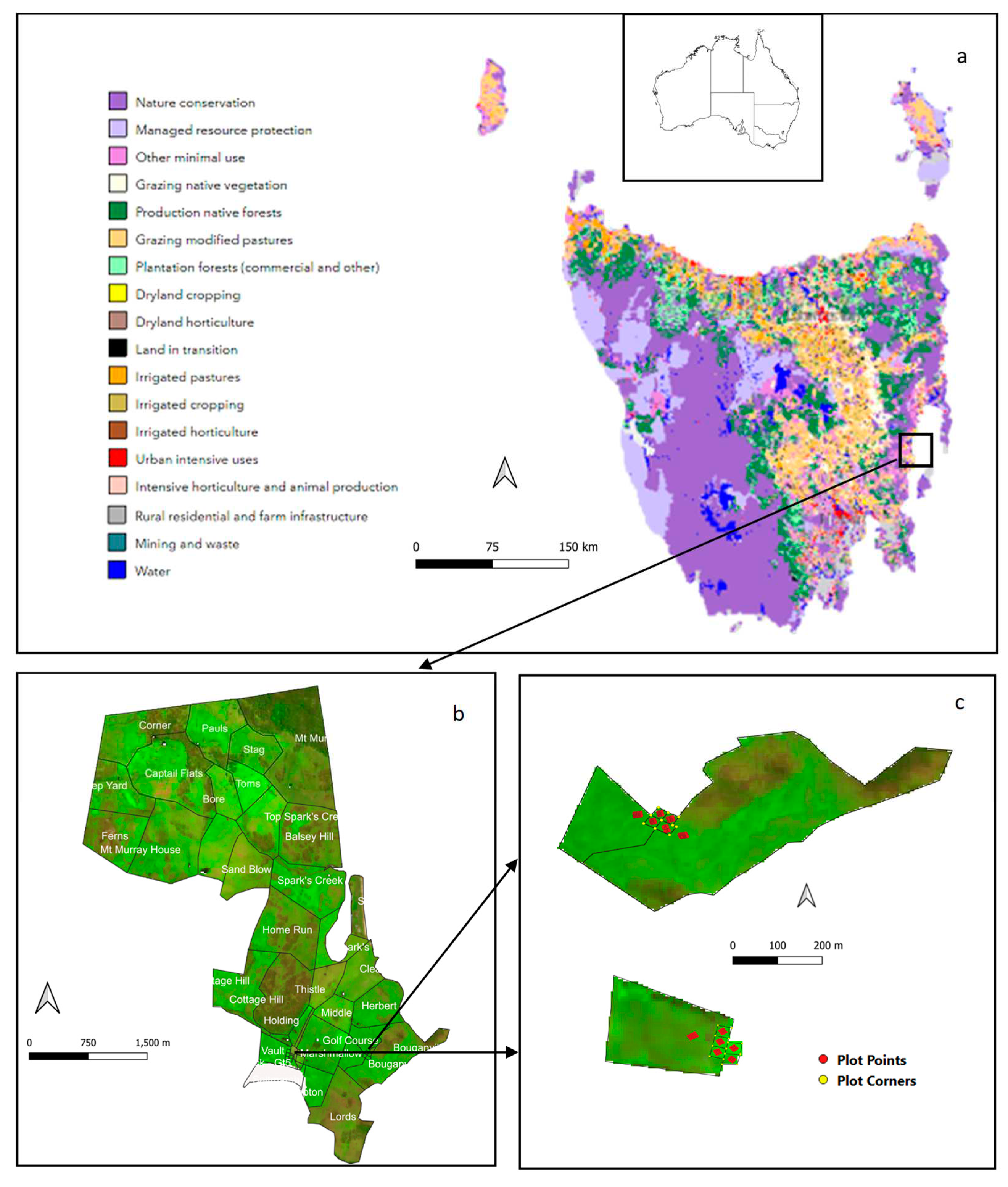
2.1. Study site
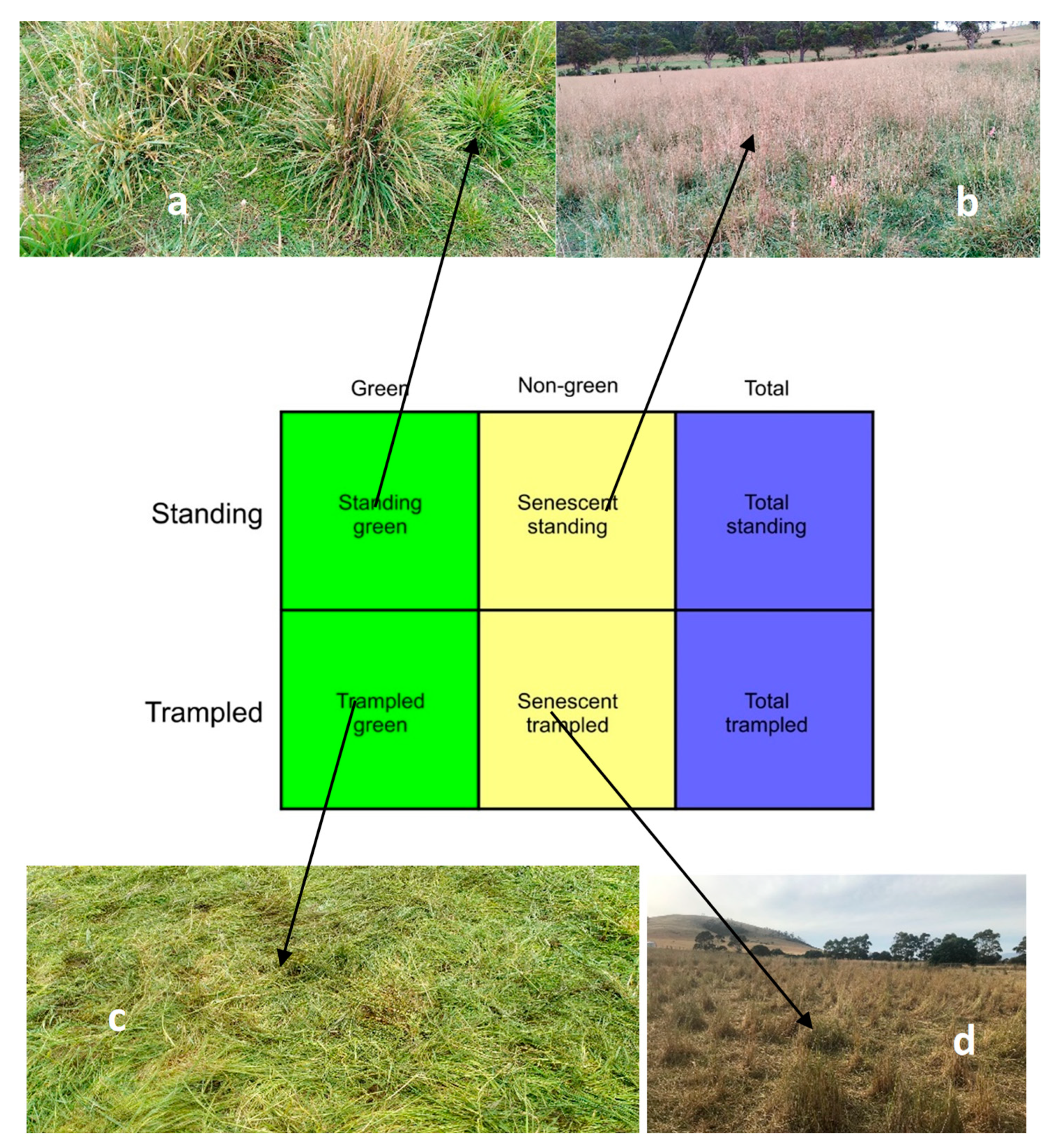
2.2. Regenerative grazing data collection
2.3. Remote sensing
2.4. Comparing measured pasture biomass with satellite estimates
3. RESULTS
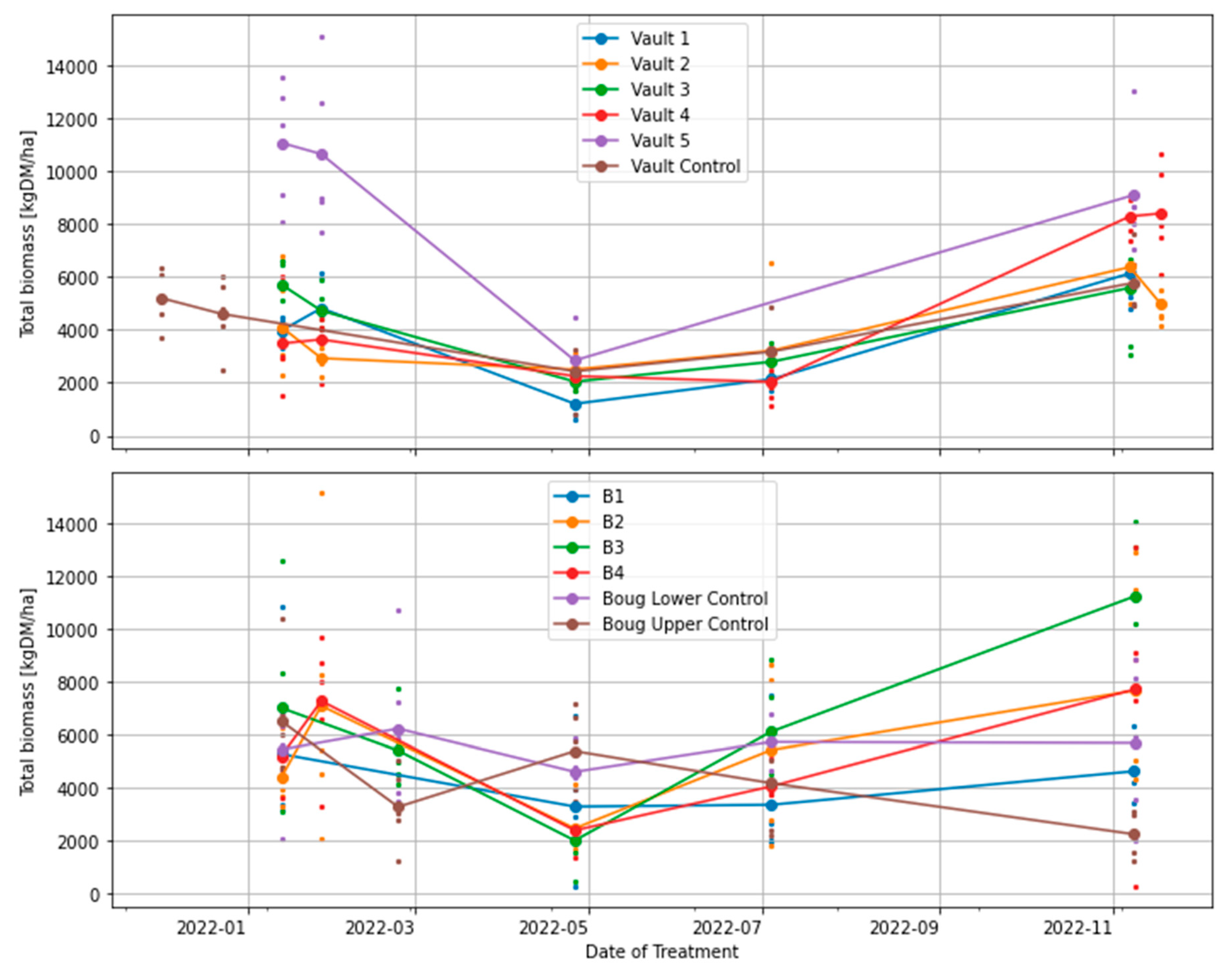
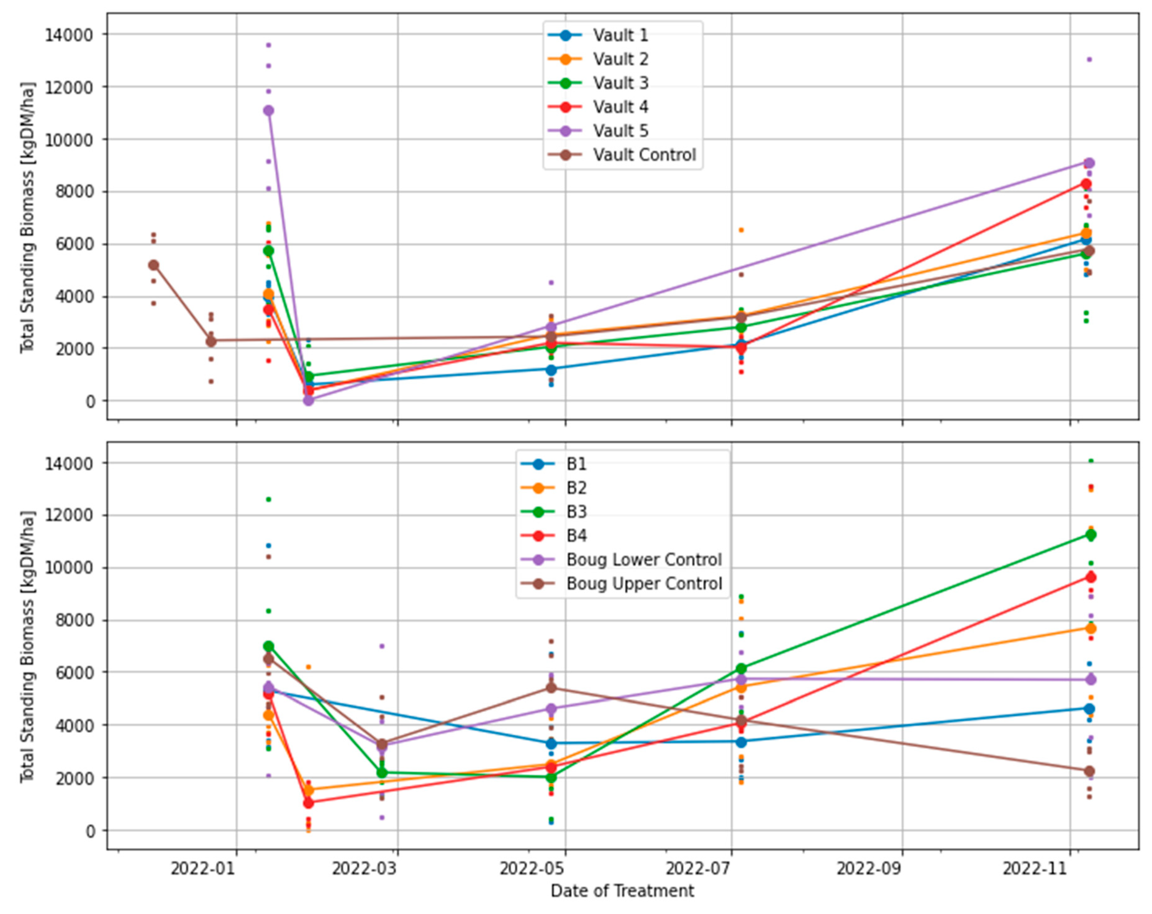
3.1. The effects of regenerative grazing on pasture productivity, consumption and trampling
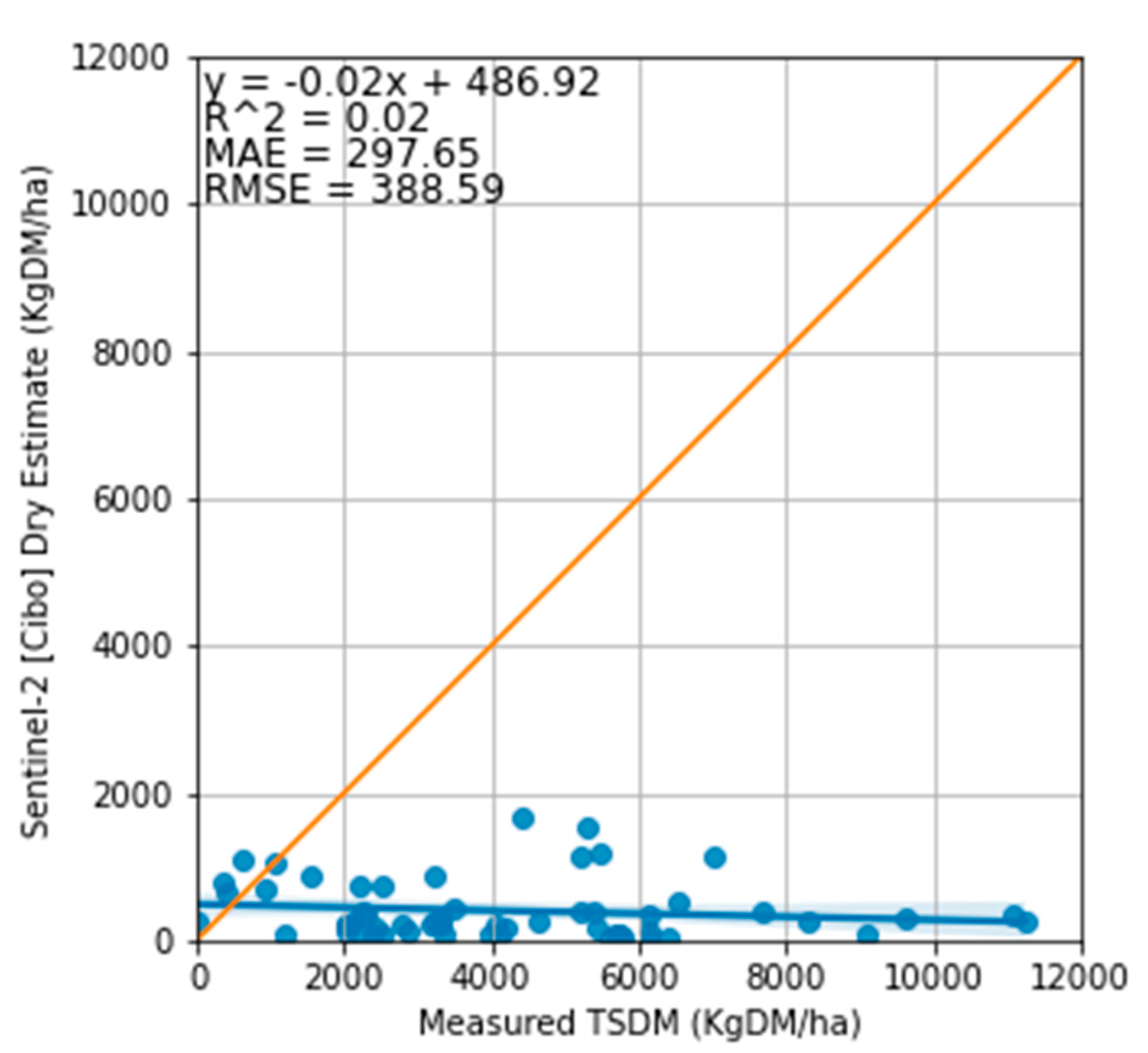
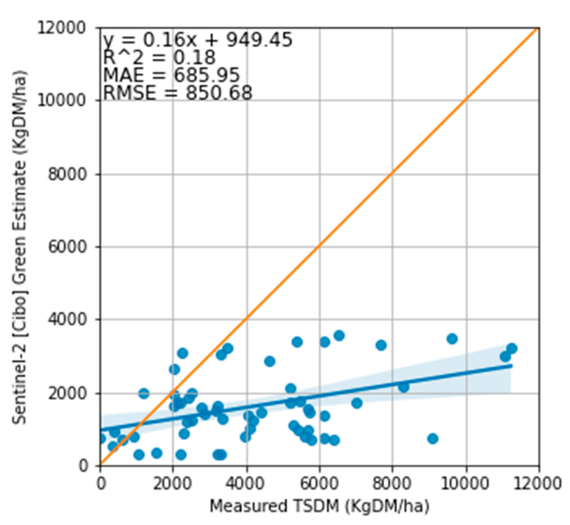
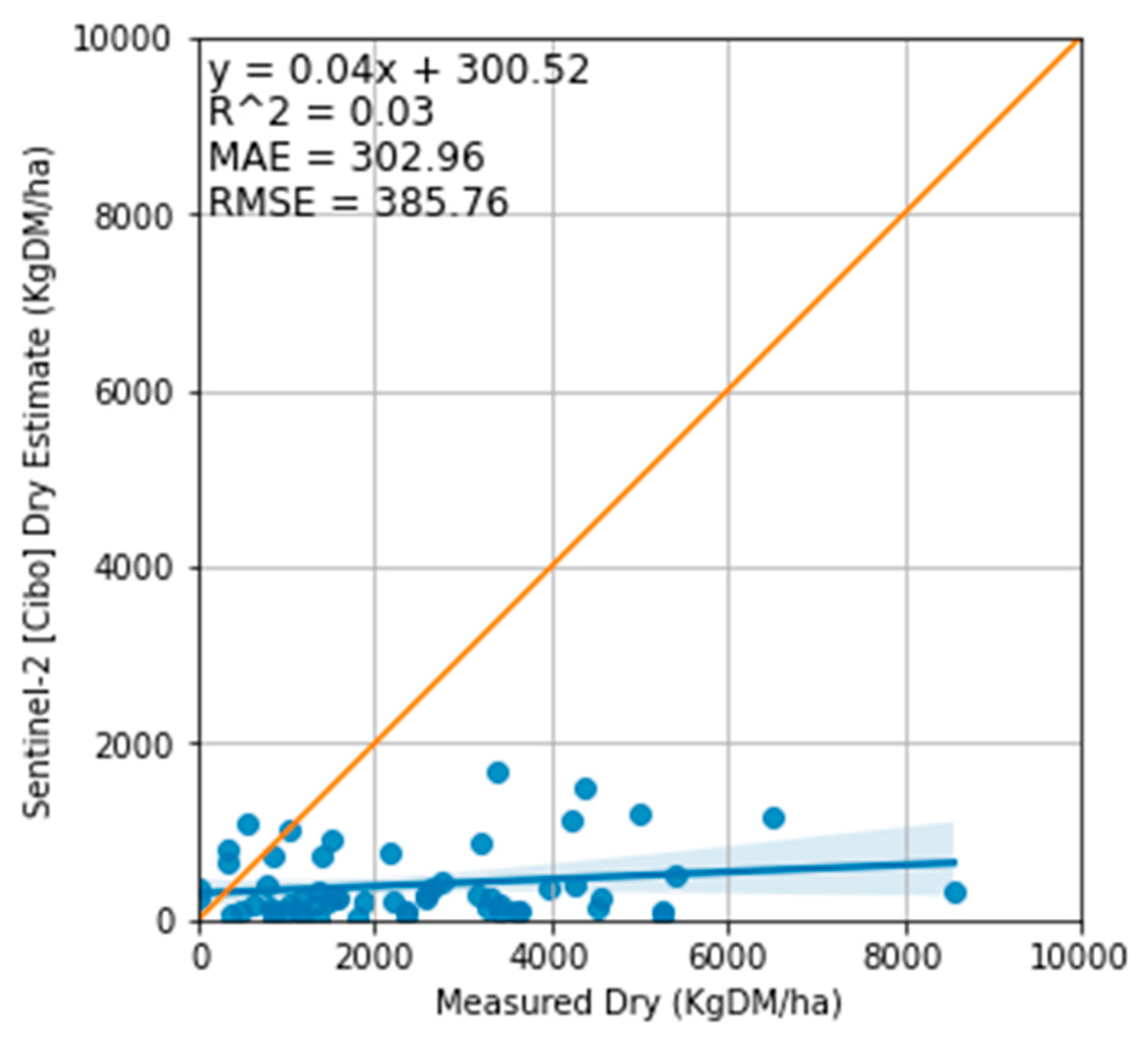
3.2. Satellite estimate of pasture biomass
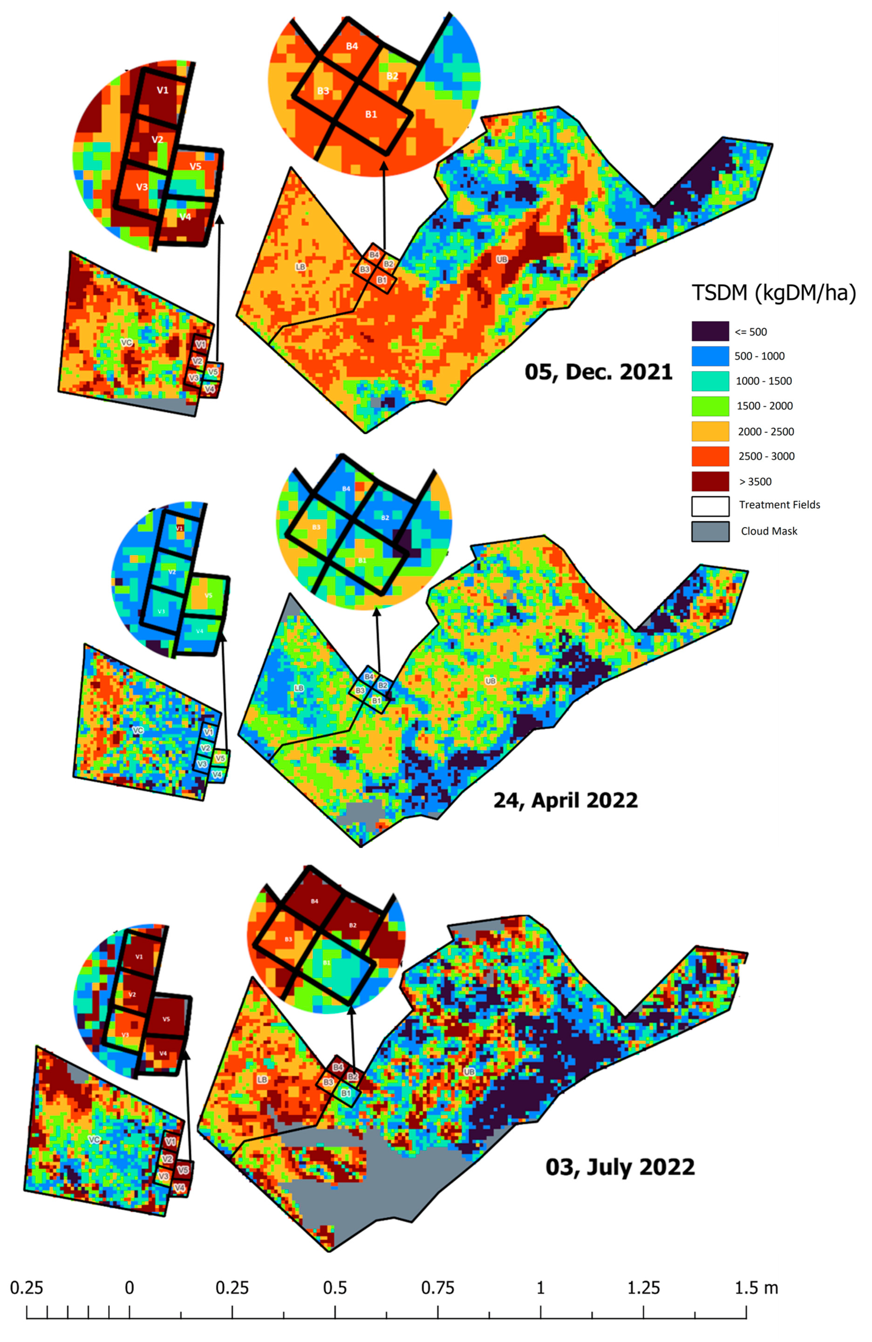
3.3. Spatial maps derived from Sentinel—2 imagery and Cibo Labs model
4. DISCUSSION
4.1. The effects of regenerative grazing on pasture biomass productivity, consumption and trampling
4.2. Satellite estimates of pasture biomass
4.3. The feasibility of using Sentinel-2 imagery to estimate total standing dry matter
5. CONCLUSION
Supplementary Materials
Author Contributions
Funding
Acknowledgments
Conflicts of Interest
References
- Harrison, M.T.; Cullen, B.R.; Mayberry, D.E.; Cowie, A.L.; Bilotto, F.; Badgery, W.B.; Liu, K.; Davison, T.; Christie, K.M.; Muleke, A.; et al. Carbon myopia: The urgent need for integrated social, economic and environmental action in the livestock sector. Glob. Chang. Biol. 2021, 27, 5726–5761. [Google Scholar] [CrossRef]
- Christie, K.M.; Smith, A.P.; Rawnsley, R.P.; Harrison, M.T.; Eckard, R.J. Simulated seasonal responses of grazed dairy pastures to nitrogen fertilizer in SE Australia: N loss and recovery. Agric. Syst. 2020, 182, 102847. [Google Scholar] [CrossRef]
- Thornton, P.K. Livestock production: recent trends, future prospects. Philos. Trans. R. Soc. London. Ser. B, Biol. Sci. 2010, 365, 2853–2867. [Google Scholar] [CrossRef]
- Farina, R.; Sándor, R.; Abdalla, M.; Álvaro-Fuentes, J.; Bechini, L.; Bolinder, M.A.; Brilli, L.; Chenu, C.; Clivot, H.; De Antoni Migliorati, M.; et al. Ensemble modelling, uncertainty and robust predictions of organic carbon in long-term bare-fallow soils. Glob. Chang. Biol. 2021, 27, 904–928. [Google Scholar] [CrossRef]
- Abberton, M. Grassland carbon sequestration : management , Proceedings of the Workshop sequestration in the mitigation of climate change. In Food and Agriculture Organisation; 2010; Vol. Vol. 11.
- Franzluebbers, A.J. Soil organic carbon in managed pastures of the southeastern United States of America. Grassl. carbon sequestration Manag. policy Econ. Proc. Work. role Grassl. carbon sequestration Mitig. Clim. Chang. 2010, 2007, 163–175. [Google Scholar]
- Henry, B.; Dalal, R.; Harrison, M.T.; Keating, B. Creating frameworks to foster soil carbon sequestration. 2022.
- Teague, R.; Kreuter, U. Managing Grazing to Restore Soil Health, Ecosystem Function, and Ecosystem Services. Front. Sustain. Food Syst. 2020, 4. [Google Scholar] [CrossRef]
- Díaz de Otálora, X.; Epelde, L.; Arranz, J.; Garbisu, C.; Ruiz, R.; Mandaluniz, N. Regenerative rotational grazing management of dairy sheep increases springtime grass production and topsoil carbon storage. Ecol. Indic. 2021, 125, 107484. [Google Scholar] [CrossRef]
- Teague, R.; Barnes, M. Grazing management that regenerates ecosystem function and grazingland livelihoods. African J. Range \& Forage Sci. 2017, 34, 77–86. [Google Scholar] [CrossRef]
- Spratt, E.; Jordan, J.; Winsten, J.; Huff, P.; van Schaik, C.; Jewett, J.G.; Filbert, M.; Luhman, J.; Meier, E.; Paine, L. Accelerating regenerative grazing to tackle farm, environmental, and societal challenges in the upper Midwest. J. Soil Water Conserv. 2021, 76, 15A–23A. [Google Scholar] [CrossRef]
- Öllerer, K.; Varga, A.; Kirby, K.; Demeter, L.; Biró, M.; Bölöni, J.; Molnár, Z. Beyond the obvious impact of domestic livestock grazing on temperate forest vegetation – A global review. Biol. Conserv. 2019, 237, 209–219. [Google Scholar] [CrossRef]
- Harrison, M.; Evans, J.; Moore, A.D. Using a mathematical framework to examine physiological changes in winter wheat after livestock grazing 2. Model validation and effects of grazing management. F. Crop. Res. 2012, 136, 127–137. [Google Scholar] [CrossRef]
- Harrison, M.T.; Evans, J.R.; Moore, A.D. Using a mathematical framework to examine physiological changes in winter wheat after livestock grazing: 1. Model derivation and coefficient calibration. F. Crop. Res. 2012, 136, 116–126. [Google Scholar] [CrossRef]
- Ara, I.; Harrison, M.T.; Whitehead, J.; Waldner, F.; Bridle, K.; Gilfedder, L.; Marques Da Silva, J.; Marques, F.; Rawnsley, R. Modelling seasonal pasture growth and botanical composition at the paddock scale with satellite imagery. In Silico Plants 2021, 3, 1–15. [Google Scholar] [CrossRef]
- Chen, Y.; Guerschman, J.; Shendryk, Y.; Henry, D.; Harrison, M.T. Estimating pasture biomass using sentinel-2 imagery and machine learning. Remote Sens. 2021, 13, 1–20. [Google Scholar] [CrossRef]
- Snow, V.; Rodriguez, D.; Dynes, R.; Kaye-Blake, W.; Mallawaarachchi, T.; Zydenbos, S.; Cong, L.; Obadovic, I.; Agnew, R.; Amery, N.; et al. Resilience achieved via multiple compensating subsystems: The immediate impacts of COVID-19 control measures on the agri-food systems of Australia and New Zealand. Agric. Syst. 2021, 187, 103025. [Google Scholar] [CrossRef]
- Phelan, D.C.; Harrison, M.T.; McLean, G.; Cox, H.; Pembleton, K.G.; Dean, G.J.; Parsons, D.; do Amaral Richter, M.E.; Pengilley, G.; Hinton, S.J.; et al. Advancing a farmer decision support tool for agronomic decisions on rainfed and irrigated wheat cropping in Tasmania. Agric. Syst. 2018, 167, 113–124. [Google Scholar] [CrossRef]
- Ibrahim, A.; Harrison, M.; Meinke, H.; Fan, Y.; Johnson, P.; Zhou, M. A regulator of early flowering in barley (Hordeum vulgare L.). PLoS One 2018, 13, e0200722. [Google Scholar] [CrossRef]
- Ara, I.; Harrison, M.T.; Whitehead, J.; Waldner, F.; Bridle, K.; Gilfedder, L.; da Silva, J.; Marques, F.; Rawnsley, R. Modelling seasonal pasture growth and botanical composition at the paddock scale with satellite imagery. in silico Plants 2020, 3. [Google Scholar] [CrossRef]
- Liu, K.; Harrison, M.T.; Shabala, S.; Meinke, H.; Ahmed, I.; Zhang, Y.; Tian, X.; Zhou, M. The State of the Art in Modeling Waterlogging Impacts on Plants: What Do We Know and What Do We Need to Know. Earth’s Futur. 2020, 8, e2020EF001801. [Google Scholar] [CrossRef]
- Ho, C.K.M.; Jackson, T.; Harrison, M.T.; Eckard, R.J. Increasing ewe genetic fecundity improves whole-farm production and reduces greenhouse gas emissions intensities: 2. Economic performance. Anim. Prod. Sci. 2014, 54, 1248–1253. [Google Scholar] [CrossRef]
- Shahpari, S.; Allison, J.; Harrison, M.T.; Stanley, R. An Integrated Economic, Environmental and Social Approach to Agricultural Land-Use Planning. Land 2021, 10. [Google Scholar] [CrossRef]
- Fayemi, P.O.; Fayemi, O.E.; Joel, L.O.; Ogungbuyi, M.G. COVID-19 Syndrome: Nexus with Herbivory and Exposure Dynamics for Monitoring Livestock Welfare and Agro-Environment. Sustainability 2021, 13. [Google Scholar] [CrossRef]
- Langworthy, A.D.; Rawnsley, R.P.; Freeman, M.J.; Pembleton, K.G.; Corkrey, R.; Harrison, M.T.; Lane, P.A.; Henry, D.A. Potential of summer-active temperate (C3) perennial forages to mitigate the detrimental effects of supraoptimal temperatures on summer home-grown feed production in south-eastern Australian dairying regions. Crop Pasture Sci. 2018, 69, 808–820. [Google Scholar] [CrossRef]
- Harrison, M.T. Climate change benefits negated by extreme heat. Nat. Food 2021, 2, 855–856. [Google Scholar] [CrossRef] [PubMed]
- Liu, K.; Harrison, M.T.; Archontoulis, S. V; Huth, N.; Yang, R.; Liu, D.L.; Yan, H.; Meinke, H.; Huber, I.; Feng, P. Climate change shifts forward flowering and reduces crop waterlogging stress. Environ. Res. Lett. 2021, 16, 94017. [Google Scholar] [CrossRef]
- Hudson, T.D.; Reeves, M.C.; Hall, S.A.; Yorgey, G.G.; Neibergs, J.S. Big landscapes meet big data: Informing grazing management in a variable and changing world. Rangelands 2021, 43, 17–28. [Google Scholar] [CrossRef]
- Trotter, M.G.; Lamb, D.W.; Donald, G.E.; Schneider, D.A. Evaluating an active optical sensor for quantifying and mapping green herbage mass and growth in a perennial grass pasture. Crop Pasture Sci. 2010, 61, 389–398. [Google Scholar] [CrossRef]
- Punalekar, S.M.; Verhoef, A.; Quaife, T.L.; Humphries, D.; Bermingham, L.; Reynolds, C.K. Application of Sentinel-2A data for pasture biomass monitoring using a physically based radiative transfer model. Remote Sens. Environ. 2018, 218, 207–220. [Google Scholar] [CrossRef]
- Edirisinghe, A.; Clark, D.; Waugh, D. Spatio-temporal modelling of biomass of intensively grazed perennial dairy pastures using multispectral remote sensing. Int. J. Appl. Earth Obs. Geoinf. 2012, 16, 5–16. [Google Scholar] [CrossRef]
- Wang, J.; Xiao, X.; Bajgain, R.; Starks, P.; Steiner, J.; Doughty, R.B.; Chang, Q. Estimating leaf area index and aboveground biomass of grazing pastures using Sentinel-1, Sentinel-2 and Landsat images. ISPRS J. Photogramm. Remote Sens. 2019, 154, 189–201. [Google Scholar] [CrossRef]
- Morais, T.G.; Teixeira, R.F.M.; Figueiredo, M.; Domingos, T. The use of machine learning methods to estimate aboveground biomass of grasslands: A review. Ecol. Indic. 2021, 130, 108081. [Google Scholar] [CrossRef]
- Harrison, M.T.; Roggero, P.P.; Zavattaro, L. Simple, efficient and robust techniques for automatic multi-objective function parameterisation: Case studies of local and global optimisation using APSIM. Environ. Model. Softw. 2019, 117, 109–133. [Google Scholar] [CrossRef]
- Ali, I.; Greifeneder, F.; Stamenkovic, J.; Neumann, M.; Notarnicola, C. Review of Machine Learning Approaches for Biomass and Soil Moisture Retrievals from Remote Sensing Data. Remote Sens. 2015, 7, 16398–16421. [Google Scholar] [CrossRef]
- Gitelson, A.A.; Gamon, J.A. The need for a common basis for defining light-use efficiency: Implications for productivity estimation. Remote Sens. Environ. 2015, 156, 196–201. [Google Scholar] [CrossRef]
- Delegido, J.; Verrelst, J.; Rivera, J.P.; Ruiz-Verdú, A.; Moreno, J. Brown and green LAI mapping through spectral indices. Int. J. Appl. Earth Obs. Geoinf. 2015, 35, 350–358. [Google Scholar] [CrossRef]
- Bsaibes, A.; Courault, D.; Baret, F.; Weiss, M.; Olioso, A.; Jacob, F.; Hagolle, O.; Marloie, O.; Bertrand, N.; Desfond, V.; et al. Albedo and LAI estimates from FORMOSAT-2 data for crop monitoring. Remote Sens. Environ. 2009, 113, 716–729. [Google Scholar] [CrossRef]
- De Rosa, D.; Basso, B.; Fasiolo, M.; Friedl, J.; Fulkerson, B.; Grace, P.R.; Rowlings, D.W. Predicting pasture biomass using a statistical model and machine learning algorithm implemented with remotely sensed imagery. Comput. Electron. Agric. 2021, 180. [Google Scholar] [CrossRef]
- Ibrahim, A.; Harrison, M.T.; Meinke, H.; Zhou, M. Examining the yield potential of barley near-isogenic lines using a genotype by environment by management analysis. Eur. J. Agron. 2019, 105, 41–51. [Google Scholar] [CrossRef]
- Zhai, Z.; Martínez, J.F.; Beltran, V.; Martínez, N.L. Decision support systems for agriculture 4.0: Survey and challenges. Comput. Electron. Agric. 2020, 170, 105256. [Google Scholar] [CrossRef]
- Ge, Y.; Thomasson, J.A.; Sui, R. Remote sensing of soil properties in precision agriculture: A review. Front. Earth Sci. 2011, 5, 229–238. [Google Scholar] [CrossRef]
- Bilotto, F.; Harrison, M.T.; Migliorati, M.D.A.; Christie, K.M.; Rowlings, D.W.; Grace, P.R.; Smith, A.P.; Rawnsley, R.P.; Thorburn, P.J.; Eckard, R.J. Can seasonal soil N mineralisation trends be leveraged to enhance pasture growth? Sci. Total Environ. 2021, 772, 145031. [Google Scholar] [CrossRef] [PubMed]
- Ali, I.; Cawkwell, F.; Dwyer, E.; Barrett, B.; Green, S. Satellite remote sensing of grasslands: From observation to management. J. Plant Ecol. 2016, 9, 649–671. [Google Scholar] [CrossRef]
- Smith, R.C.G.; Adams, M.; Gittins, S.; Gherardi, S.; Wood, D.; Maier, S.; Stovold, R.; Donald, G.; Khohkar, S.; Allen, A. Near real-time Feed On Offer (FOO) from MODIS for early season grazing management of Mediterranean annual pastures. Int. J. Remote Sens. 2011, 32, 4445–4460. [Google Scholar] [CrossRef]
- Dingaan, M.N. V; Tsubo, M. Improved assessment of pasture availability in semi-arid grassland of South Africa. Environ. Monit. Assess. 2019, 191. [Google Scholar] [CrossRef] [PubMed]
- Guerschman, J.P.; Hill, M.J.; Renzullo, L.J.; Barrett, D.J.; Marks, A.S.; Botha, E.J. Estimating fractional cover of photosynthetic vegetation, non-photosynthetic vegetation and bare soil in the Australian tropical savanna region upscaling the EO-1 Hyperion and MODIS sensors. Remote Sens. Environ. 2009, 113, 928–945. [Google Scholar] [CrossRef]
- Zhang, B.; Carter, J. FORAGE – An online system for generating and delivering property-scale decision support information for grazing land and environmental management. Comput. Electron. Agric. 2018, 150, 302–311. [Google Scholar] [CrossRef]
- Dong, S.; Shang, Z.; Gao, J.; Boone, R.B. Enhancing sustainability of grassland ecosystems through ecological restoration and grazing management in an era of climate change on Qinghai-Tibetan Plateau. Agric. Ecosyst. Environ. 2020, 287. [Google Scholar] [CrossRef]
- Donnelly, J.R.; Moore, A.D.; Freer, M. GRAZPLAN: Decision support systems for Australian grazing enterprises—I. Overview of the GRAZPLAN project, and a description of the MetAccess and LambAlive DSS. Agric. Syst. 1997, 54, 57–76. [Google Scholar] [CrossRef]
- Srivastava, N.; Hinton, G.; Krizhevsky, A.; Sutskever, I.; Salakhutdinov, R. Dropout: A simple way to prevent neural networks from overfitting. J. Mach. Learn. Res. 2014, 15, 1929–1958. [Google Scholar]
- Verrelst, J.; Malenovský, Z.; Van der Tol, C.; Camps-Valls, G.; Gastellu-Etchegorry, J.-P.; Lewis, P.; North, P.; Moreno, J. Quantifying Vegetation Biophysical Variables from Imaging Spectroscopy Data: A Review on Retrieval Methods. Surv. Geophys. 2019, 40, 589–629. [Google Scholar] [CrossRef]
- CRCSI Earth Observation: Data, Processing and Applications. Volume 1A: Data—Basics and Acquisition; Melbourne, Australia, 2018.
- Scarth, P.; Armston, J.; Flood, N.; Denham, R.; Collett, L.; Watson, F.; Trevithick, B.; Muir, J.; Goodwin, N.; Tindalla, D.; et al. OPERATIONAL APPLICATION OF THE LANDSAT TIMESERIES TO ADDRESS LARGE AREA LANDCOVER UNDERSTANDING. Int. Arch. Photogramm. Remote Sens. Spat. Inf. Sci. 2015, XL-3-W3, 571–575. [CrossRef]
- Roberts, D.; Mueller, N.; Mcintyre, A. High-Dimensional Pixel Composites From Earth Observation Time Series. IEEE Trans. Geosci. Remote Sens. 2017, 55, 6254–6264. [Google Scholar] [CrossRef]
- BoM Australia Government. Bureau of meteorology. Available online: http://www.bom.gov.au/climate/averages/tables/cw_092027.shtml (accessed on Oct 25, 2022).
- Macquarie Franklin Okehampton-optimising management of production and biodiversity assets, Devonport TAS; 2019.
- Zhu, Z.; Wang, S.; Woodcock, C.E. Improvement and expansion of the Fmask algorithm: cloud, cloud shadow, and snow detection for Landsats 4–7, 8, and Sentinel 2 images. Remote Sens. Environ. 2015, 159, 269–277. [Google Scholar] [CrossRef]
- Piñeiro, G.; Perelman, S.; Guerschman, J.P.; Paruelo, J.M. How to evaluate models: Observed vs. predicted or predicted vs. observed? Ecol. Modell. 2008, 216, 316–322. [Google Scholar] [CrossRef]
- Zhu, Q.; Lin, H. Influences of soil, terrain, and crop growth on soil moisture variation from transect to farm scales. Geoderma 2011, 163, 45–54. [Google Scholar] [CrossRef]
- Warren, S.D.; Thurow, T.L.; Blackburn, W.H.; Garza, N.E. The influence of livestock trampling under intensive rotation grazing on soil hydrologic characteristics. Rangel. Ecol. Manag. Range Manag. Arch. 1986, 39, 491–495. [Google Scholar] [CrossRef]
- Khatri-Chhetri, U.; Thompson, K.A.; Quideau, S.A.; Boyce, M.S.; Chang, S.X.; Kaliaskar, D.; Bork, E.W.; Carlyle, C.N. Adaptive multi-paddock grazing increases soil nutrient availability and bacteria to fungi ratio in grassland soils. Appl. Soil Ecol. 2022, 179, 104590. [Google Scholar] [CrossRef]
- van Eekeren, N.; Jongejans, E.; van Agtmaal, M.; Guo, Y.; van der Velden, M.; Versteeg, C.; Siepel, H. Microarthropod communities and their ecosystem services restore when permanent grassland with mowing or low-intensity grazing is installed. Agric. Ecosyst. Environ. 2022, 323, 107682. [Google Scholar] [CrossRef]
- Zwerts, J.A.; Prins, H.H.T.; Bomhoff, D.; Verhagen, I.; Swart, J.M.; de Boer, W.F. Competition between a Lawn-Forming Cynodon dactylon and a Tufted Grass Species Hyparrhenia hirta on a South-African Dystrophic Savanna. PLoS One 2015, 10, e0140789. [Google Scholar] [CrossRef]
- Ivanov, V.Y.; Bras, R.L.; Vivoni, E.R. file:///C:/Users/mgo/Downloads/sustainability-v13-i22_20230426.bib. Water Resour. Res. 2008, 44. [Google Scholar] [CrossRef]
- Barrachina, M.; Cristóbal, J.; Tulla, A.F. Estimating above-ground biomass on mountain meadows and pastures through remote sensing. Int. J. Appl. Earth Obs. Geoinf. 2015, 38, 184–192. [Google Scholar] [CrossRef]
- Andresen, J.A.; Alagarswamy, G.; Rotz, C.A.; Ritchie, J.T.; LeBaron, A.W. Weather Impacts on Maize, Soybean, and Alfalfa Production in the Great Lakes Region, 1895–1996. Agron. J. 2001, 93, 1059–1070. [Google Scholar] [CrossRef]
- Edirisinghe, A.; Hill, M.J.; Donald, G.E.; Hyder, M. Quantitative mapping of pasture biomass using satellite imagery. Int. J. Remote Sens. 2011, 32, 2699–2724. [Google Scholar] [CrossRef]
- Myrgiotis, V.; Harris, P.; Revill, A.; Sint, H.; Williams, M. Inferring management and predicting sub-field scale C dynamics in UK grasslands using biogeochemical modelling and satellite-derived leaf area data. Agric. For. Meteorol. 2021, 307, 108466. [Google Scholar] [CrossRef]
- Moore, C.E.; Beringer, J.; Donohue, R.J.; Evans, B.; Exbrayat, J.-F.; Hutley, L.B.; Tapper, N.J. Seasonal, interannual and decadal drivers of tree and grass productivity in an Australian tropical savanna. Glob. Chang. Biol. 2018, 24, 2530–2544. [Google Scholar] [CrossRef]
- Segarra, J.; Buchaillot, M.L.; Araus, J.L.; Kefauver, S.C. Remote Sensing for Precision Agriculture: Sentinel-2 Improved Features and Applications. Agronomy 2020, 10. [Google Scholar] [CrossRef]
- Crabbe, R.A.; Lamb, D.W.; Edwards, C.; Andersson, K.; Schneider, D. A Preliminary Investigation of the Potential of Sentinel-1 Radar to Estimate Pasture Biomass in a Grazed Pasture Landscape. Remote Sens. 2019, 11. [Google Scholar] [CrossRef]
- Sadeh, Y.; Zhu, X.; Dunkerley, D.; Walker, J.P.; Zhang, Y.; Rozenstein, O.; Manivasagam, V.S.; Chenu, K. Fusion of Sentinel-2 and PlanetScope time-series data into daily 3 m surface reflectance and wheat LAI monitoring. Int. J. Appl. Earth Obs. Geoinf. 2021, 96, 102260. [Google Scholar] [CrossRef]
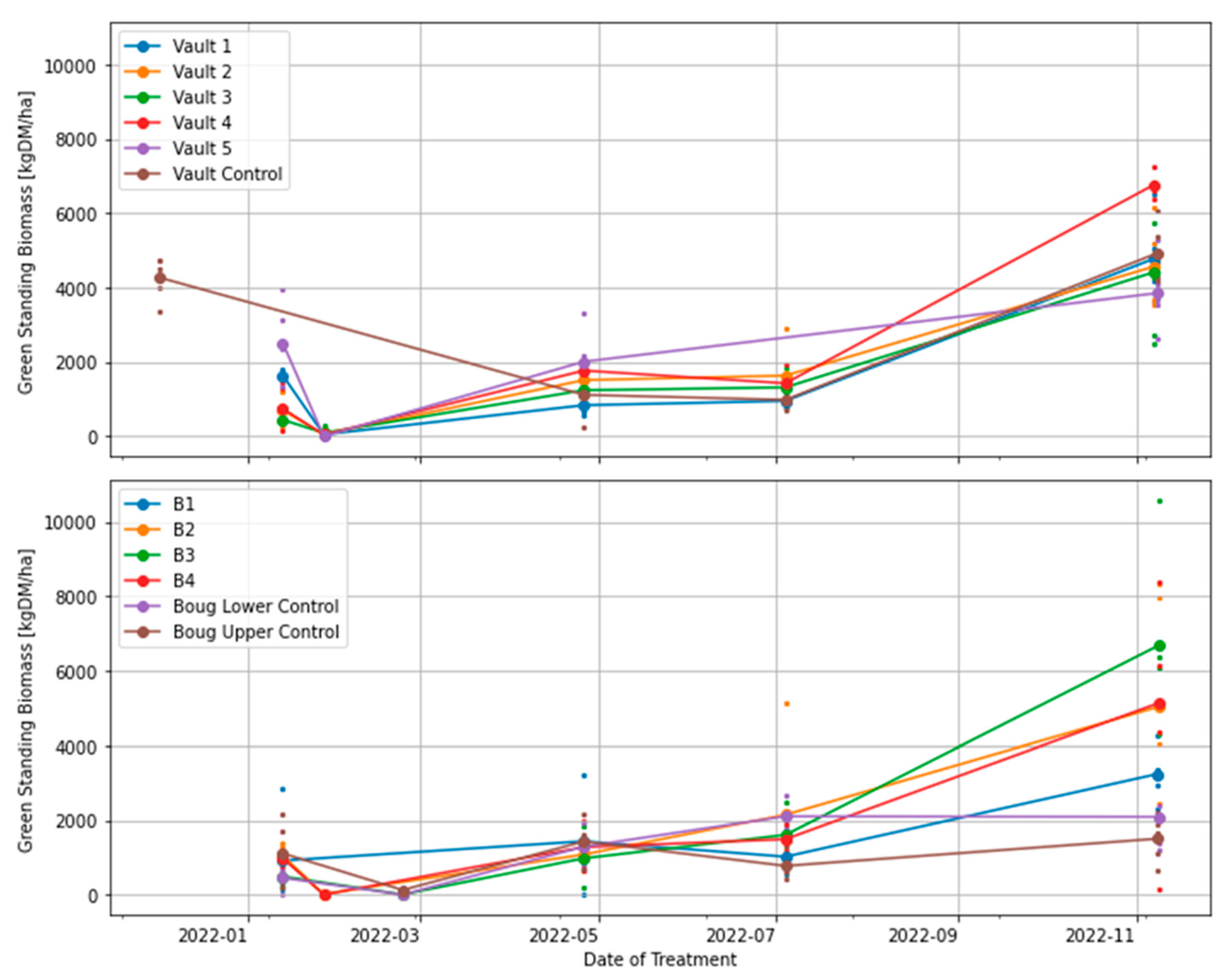
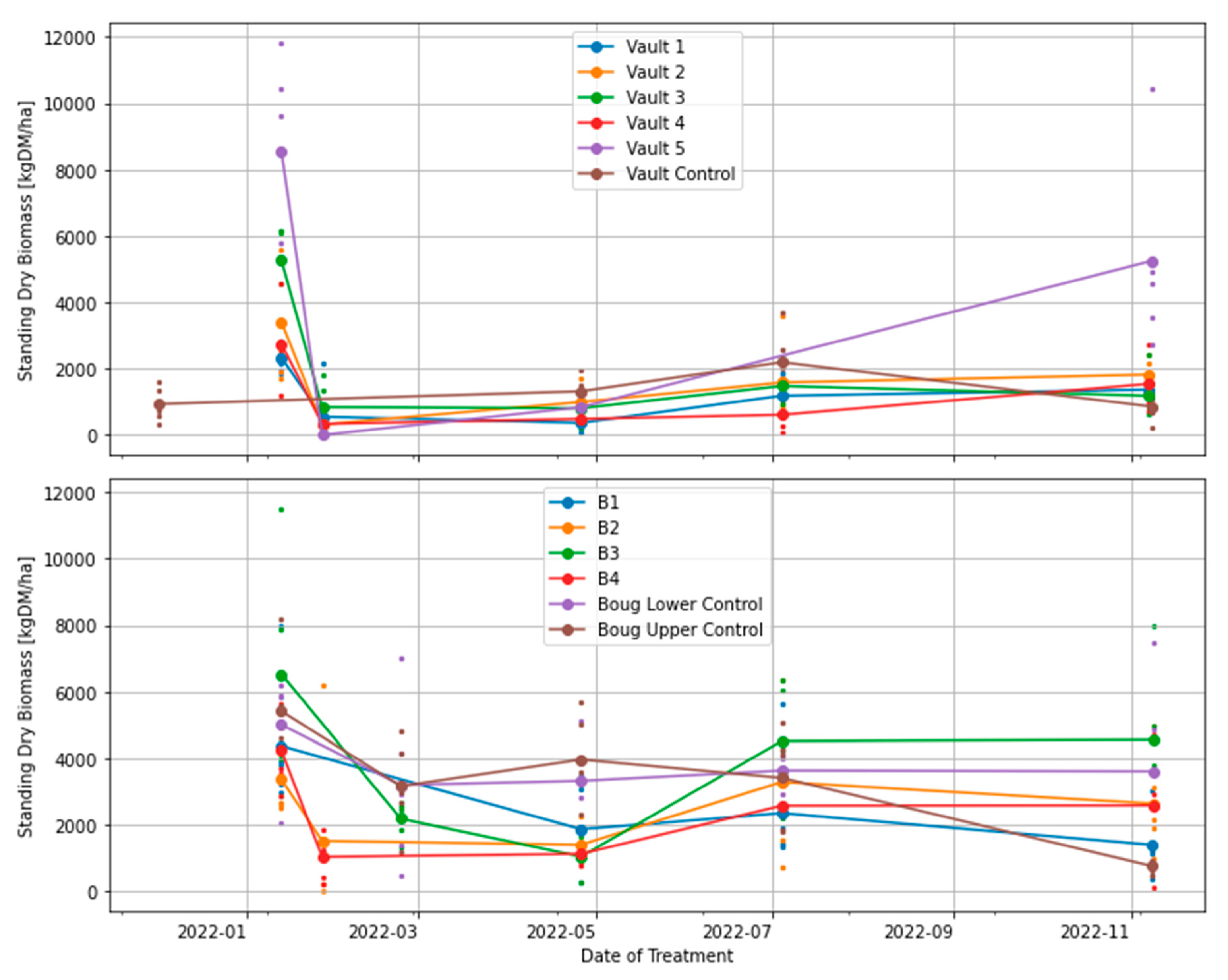
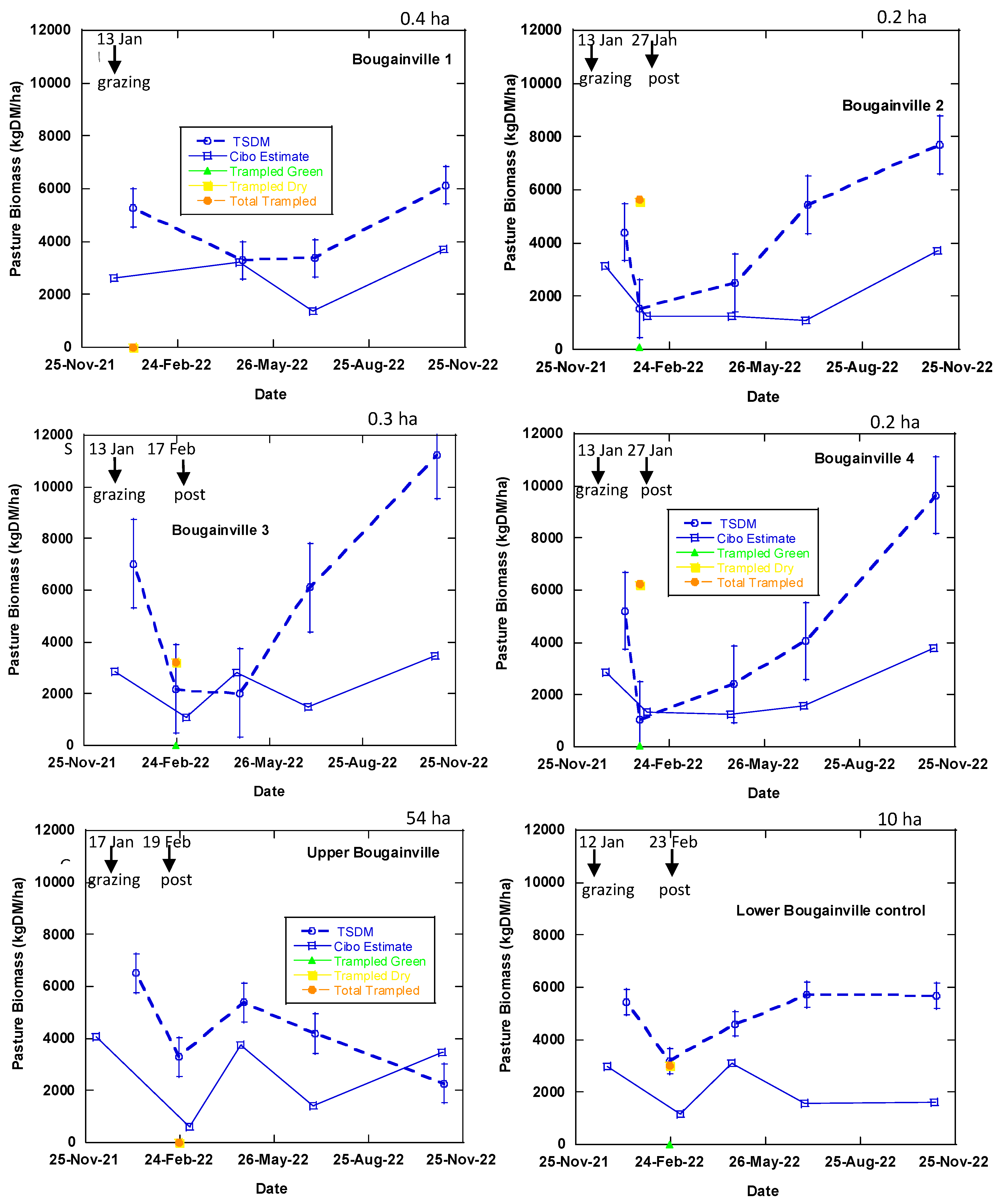
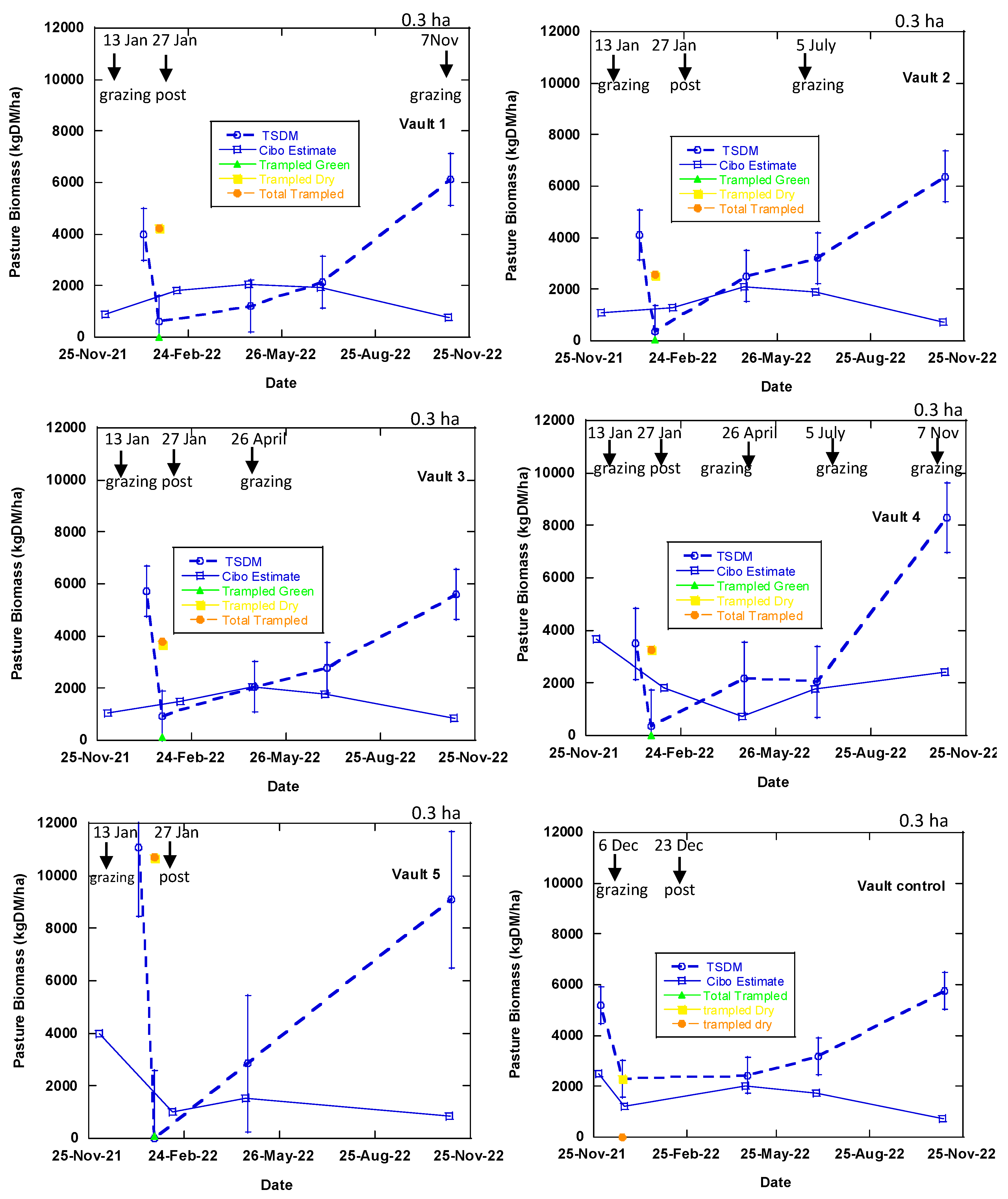
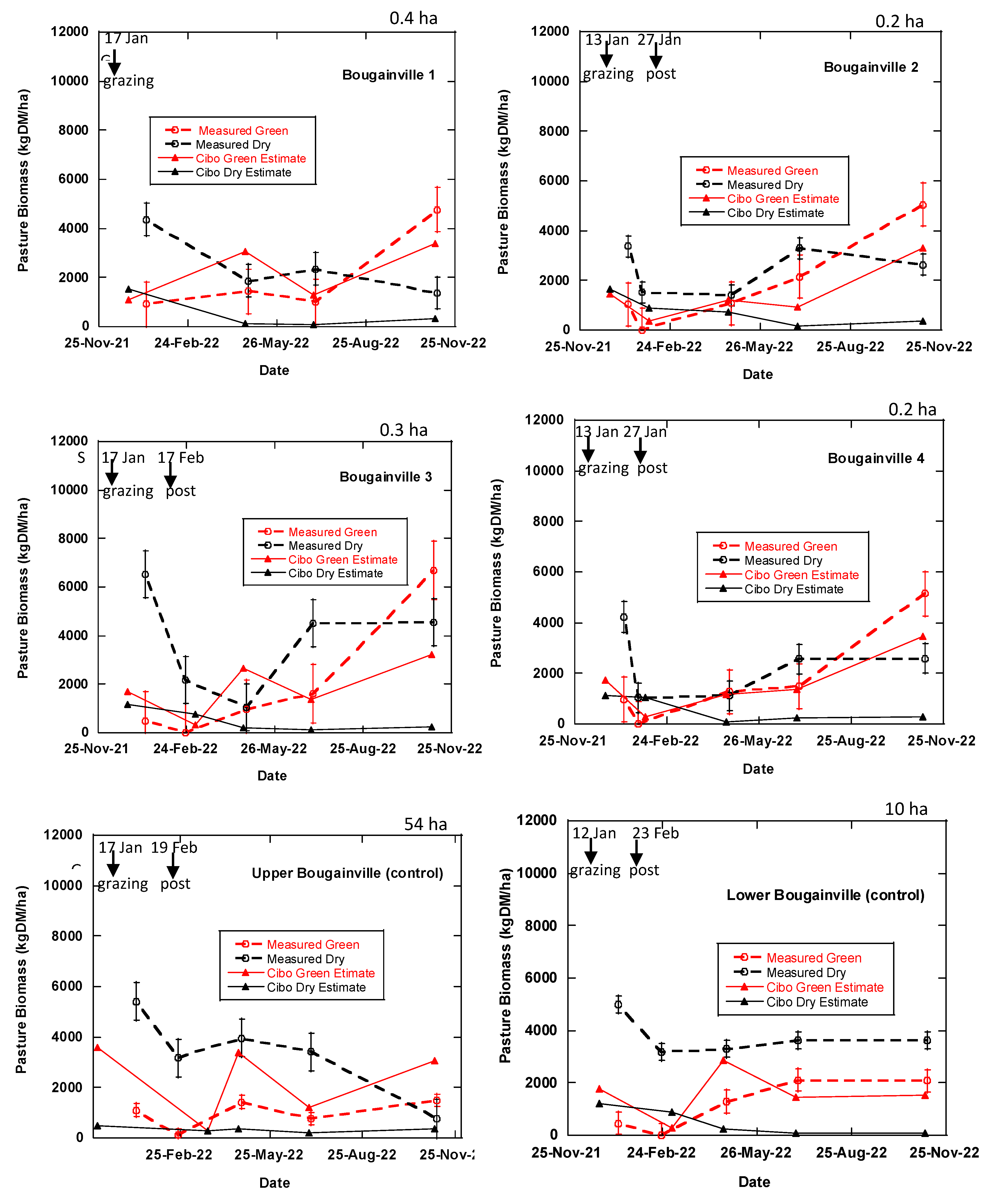
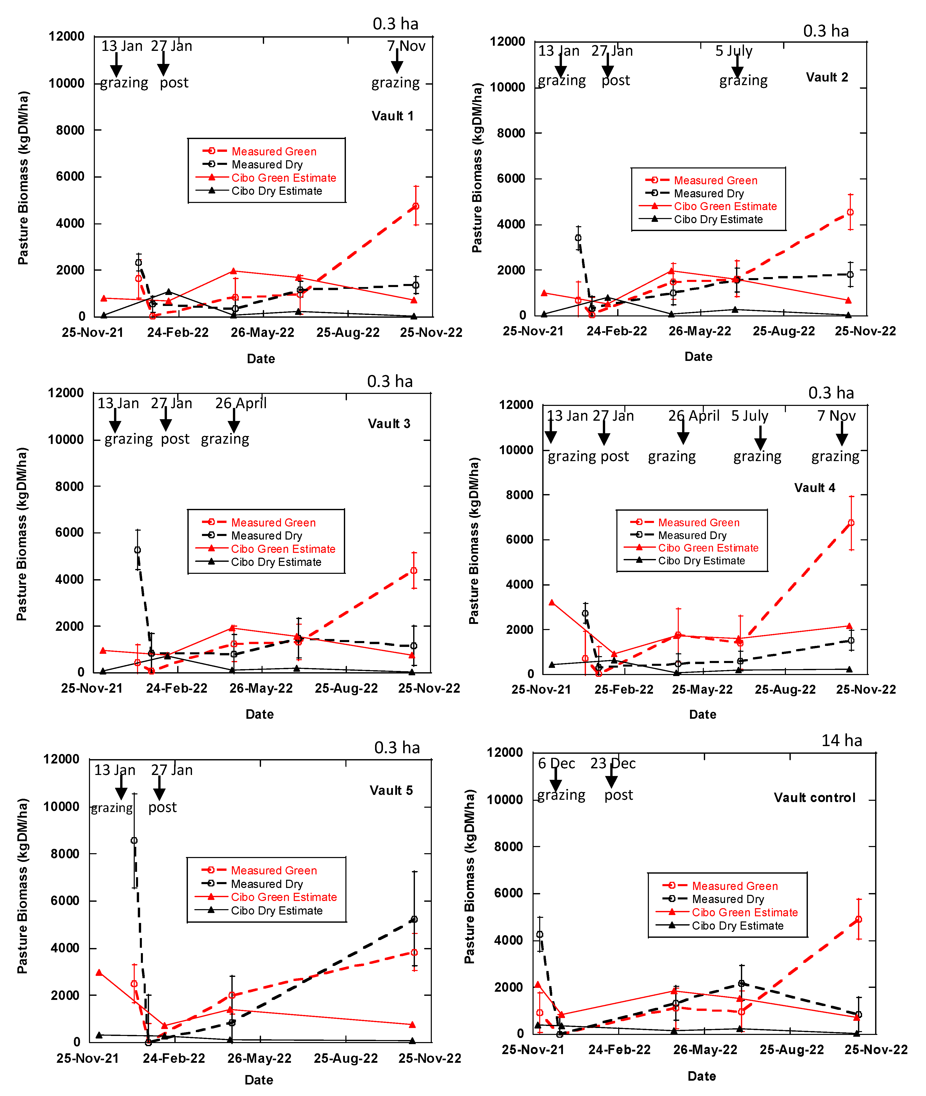
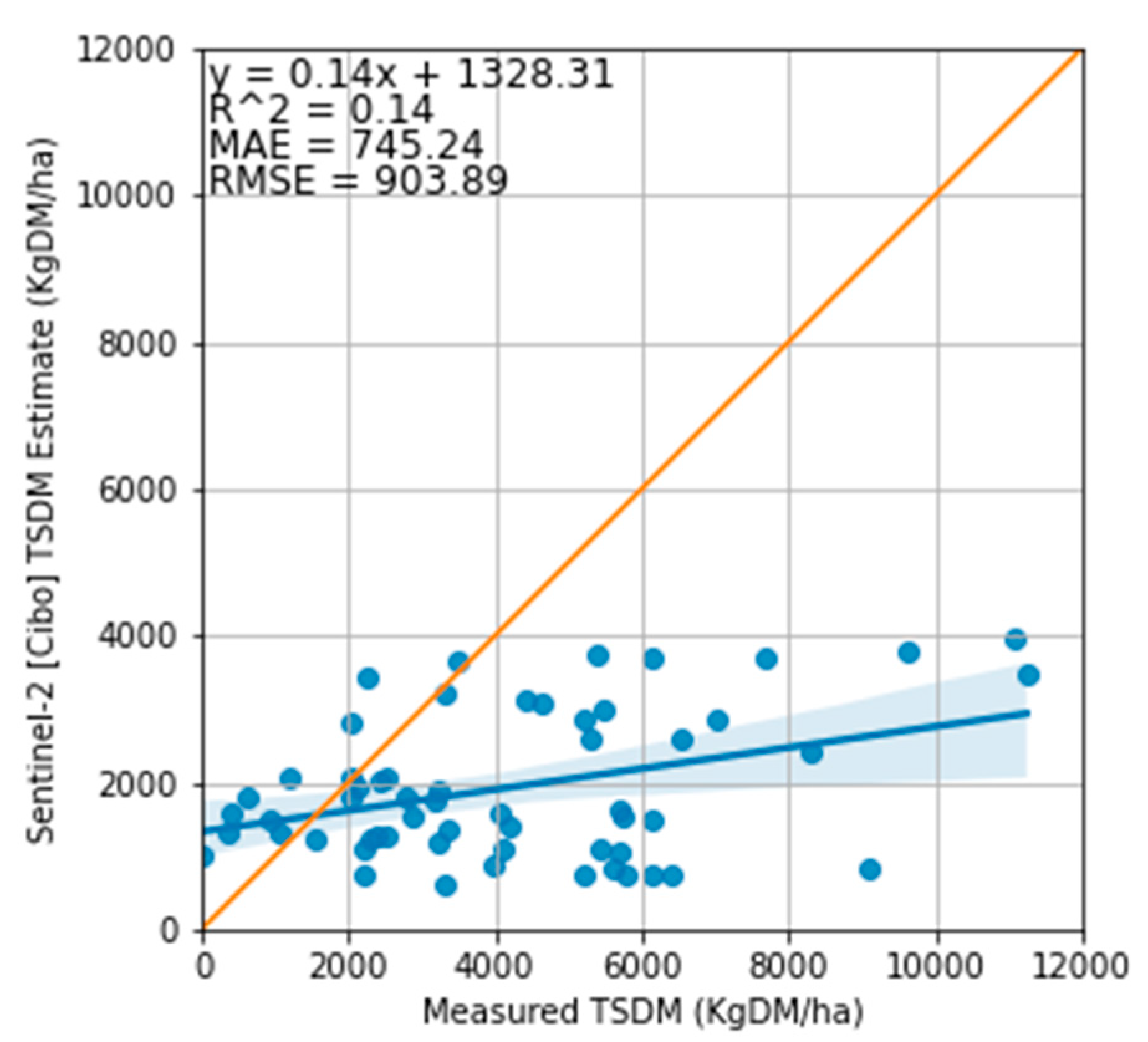
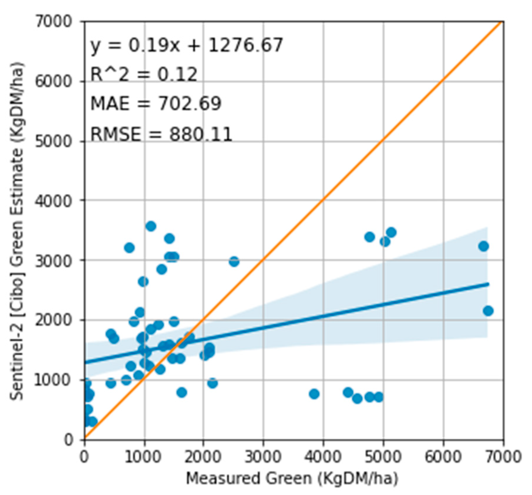
| Treatments | Plot | Phase 1 | Phase 2 | Phase 3 | Phase 4 | ||
| Size (ha) | Dec 2021 & Jan 2022 | Apr-22 | Jul-22 | Nov-22 | |||
| Grazing | Pre | Post | pre | pre | pre | ||
| Trampled after post-grazing | ✓ | V4 | |||||
| Stocking rate (DSE/ha) | 8000 | 6000 | 8800 | 8800 | |||
| BUA & Regenerative | Bougainville 1 (B1) | 0.4 | ✓ | ✓ | |||
| Regenerative | Bougainville (B2) | 0.2 | ✓ | ✓ | |||
| BUA & Regenerative | Bougainville (B3) | 0.3 | ✓ | ✓ | |||
| Regenerative | Bougainville (B4) | 0.2 | ✓ | ✓ | |||
| Control | Upper Bougainville (UB) | 54 | Business as usual | ||||
| Control | Lower Bougainville (LB) | 10 | Business as usual | ||||
| Regenerative | Vault 1 [12 months] | 0.3 | ✓ | ✓ | ✓ | ||
| Vault 2 [9 months] | 0.3 | ✓ | ✓ | ✓ | |||
| Vault 3 [6 months] | 0.3 | ✓ | ✓ | ✓ | |||
| Vault 4 [3 months] | 0.3 | ✓ | ✓ | ✓ | ✓ | ✓ | |
| Vault 5 [15 months] | 0.3 | ✓ | ✓ | ||||
| Control | Vault Control | 14 | Business as usual | ||||
Disclaimer/Publisher’s Note: The statements, opinions and data contained in all publications are solely those of the individual author(s) and contributor(s) and not of MDPI and/or the editor(s). MDPI and/or the editor(s) disclaim responsibility for any injury to people or property resulting from any ideas, methods, instructions or products referred to in the content. |
© 2023 by the authors. Licensee MDPI, Basel, Switzerland. This article is an open access article distributed under the terms and conditions of the Creative Commons Attribution (CC BY) license (http://creativecommons.org/licenses/by/4.0/).


