1. Introduction
The generation of photovoltaic energy has been one of the most developed renewable energy solutions in the world and in Chile during the last decades. It seeks to increase its presence in electrical distribution systems for industrial and residential consumption, thus satisfying the demand, and contributing to reducing the amount of CO
2 emissions into the atmosphere [
1].
The growth in the use of photovoltaic energy has encouraged the development of short-term predictive techniques to monitor the EAE produced in solar plants. However, the main difficulty in the production of photovoltaic energy is the intermittent volatility of the energy generation of the photovoltaic system, which is mainly due to the weather conditions that occur in the place where the solar plants are located. This power imbalance in the photovoltaic system can cause significant economic losses in large solar plants.
Solar plants generate daily records of the EAE produced by the photovoltaic panels. Generally, these plants have meteorological stations that generate records of the weather variables they capture. With all this data, solar plants can monitor their production and explore the incidence or correlation of the EAE produced concerning the weather conditions in the area where they operate. However, many of these solar plants do not have systems that use this data to generate models that allow them to forecast their EAE production.
The weather has a great influence on the behavior and operation of sectors such as energy, specifically in the area of photovoltaic energy. That's why the use of weather data has become an important complement to the analysis of EAE generation. Photovoltaic generators have a strong relationship with solar radiation and outdoor temperature in this energy generation process.
Meteorological variables are volatile and uncertain by nature, so unexpected changes in these parameters produce variations in the output power of photovoltaic generators. Although many researchers have focused in recent years on the development of innovative models to predict weather variables involved in the generation of photovoltaic energy, they do not commonly consider an important step such as the exploratory analysis of the data before being used [
2,
3].
There are several works aimed at predicting the generation of photovoltaic energy. However, each has particularities that vary between input variables, models to be used, data set, among others. The trend in the use of techniques from the area of machine learning in this type of forecast tasks corresponds to ANNs, particularly RNNs. This is due to the fact that the RNNs process data in time series efficiently and in which weather data can be integrated [
3].
Comparative studies of RNNs with different structural configurations, input hyperparameters and prediction horizon have been observed in the literature. However, predicting the production of photovoltaic energy with a high degree of precision is not an easy task, it requires an appropriate incorporation of weather variables and in some cases, other factors that may directly affect such as; the state of the photovoltaic panels, their calibration level, as well as components that indirectly affect such as the sensors of the weather stations, location of these stations, among other factors [
2].
Extreme weather conditions can cause intermittent and random volatility in photovoltaic systems, making photovoltaic energy forecasts difficult. An RNN is considered a powerful tool for forecasting time series data. However, when the weather strongly changes the long-term multivariate sequence, it can cause the gradient to disappear during training of an RNN, which can lead to local optimum forecast results.
The short-term memory network (LSTM) is one of the commonly used deep learning units of an RNN. Due to its particular hidden layer unit structure, it can retain the trend information contained in the long-term sequence, which allows solving RNN problems and improving its performance. An improvement to this type of LSTM unit is the gated recurrent unit (GRU) structure [
7].
Forecast of photovoltaic energy generation is important for reliable and efficient operation. Improving the accuracy of its short-term forecasts can effectively support the quality of the operational schedule of solar plants, provide a reference for photovoltaic maintenance and effective response to emergency situations. Common data sources for these types of forecasts are; recent weather records, numerical weather predictions and historical records of the EAE produced in the solar plant [
2,
3,
5,
6].
A forecast system can support the electrical operators of solar plants to balance the generation and demand of photovoltaic energy, optimize their production process, and anticipate meteorological phenomena that directly affect photovoltaic energy generation, such as sudden changes in solar radiation levels. This can help ensure that sufficient power capacity is available to cover electrical consumption requirements.
In this line of argument, in this article models are presented that forecast the weekly photovoltaic energy production of a solar plant, with multiple input variables and different hyperparameter configurations. The input variables correspond to historical records of photovoltaic energy produced in a year by the solar plant, together with records of weather variables measured in the same period, such as solar radiation, temperature, and wind speed. The hyperparameters are related to the internal components of the model, such as activation function and loss function, among others. These models are generated using a base architecture designed and described in [
7], which consists of a hybrid RNN-ANN architecture with two hidden layers. The first layer contains neurons with LSTM or GRU recurrent units, and the second layer contains shallow neurons with multi-layer perceptron (MLP) structure.
Two types of models are generated, firstly 6 models that receive the EAE records with weather variables as input. Secondly, 8 models that only receive the weather variables as input. Subsequently, these models are subjected to assessment applying different metrics and adjustments, through the development of controlled experiments under different configurations of hyperparameters. Finally, a comparison is made between the two models with the best performance of each type, achieving remarkable results. However, the models that use the EAE records as input, in addition to weather variables, stand out in their performance since in most of the metrics they obtain better results.
The article is structured as follows: the section related works describe a literature review of the last 5 years that have a direct approach to this work. The latter allows us to corroborate the innovation of the work carried out, the use of appropriate techniques and metrics. Then, the materials and method section describe the origin of the data, the methodology used, the preliminary analysis of the data, as well as its preparation and transformation. Additionally, the tool built and used to automate the entire process of design and generation of predictive models is explained. The proposed section of RNN-ANN models presents the model design, hyperparameter configuration, and metrics used for their assessment. Subsequently, the section analysis of experimental results provides a discussion of the results obtained through the selected models and performs a comparative analysis. Finally, the article ends by stating the respective conclusions obtained from the work carried out, as well as the projection of future work.
2. Related Works
The worldwide growth in the use of photovoltaic energy has spurred the development of various research initiatives aimed at obtaining high-precision to forecast models of photovoltaic energy generation. Due to the above, this research work begins with a literature review of related works in this field over the last few years to confirm the trends in the use of methodologies, technologies, and techniques.
Yesilbudak et al. [
3] describe a bibliographic review on a methodology of the data mining process for the forecast of electricity generation in solar plants. They present, in a general way, the process of extracting knowledge from the information in a database. As a result, they present a table with different investigations that are referenced and indicate the input data they use, as well as the model used in the prediction. Many of the works analyzed use ANN techniques.
The work “Analysis of Artificial Neural Networks for Forecasting Photovoltaic Energy Generation with Solar Irradiance” [
8], evaluates the forecast accuracy of the global horizontal irradiance (GHI), which is often used for short-term forecasts of solar radiation. The study uses ANN models with different construction structures and input weather variables to forecast photovoltaic energy production across three short-term forecast horizons, based on a single database. The analyses are conducted in a controlled experimental environment. The results indicate that ANNs using the GHI input variable provide higher accuracy (approximately 10%), while its absence increases error variability. No significant differences
were identified in the forecast error models trained with different input data sets. Furthermore, forecast errors were similar for the same ANN model across different forecast horizons. The 30 and 60 neuron models with one hidden layer demonstrated similar or higher accuracy compared to those with two hidden layers.
In [
9], a study is described that utilizes a time-frequency analysis based on short waveforms of data, combined with RNN, to predict solar irradiation in the next 10 minutes and calculate the generation of photovoltaic energy. The validation results of this study indicate that the proposed predictor model has a deviation of less than 4% in 90.60% of sample days analyzed. The MSE of the final model improves accuracy by 37.52% compared to the persistence reference model.
In the research conducted by Carrera et al. in [
10], it is stated that the most common data sources for forecasting of generation photovoltaic energy, are recent weather records and numerical weather forecasts. This work proposes suitable RNNs that can use each data source or both. Focusing on a 24-hour-ahead forecast problem, the authors first design two RNNs for the forecast: one for deep-forward that uses weather forecast data and a second that uses recent weather observations. Finally, a hybrid network, called PVHybNet, combines both networks to improve forecast performance. The final model predicts photovoltaic energy generation from the Yeongam Solar Plant in South Korea with an
value of 92.7%. The results support the effectiveness of the combined network using recent weather observations and weather forecasts. The authors also demonstrate that the hybrid model outperforms various machine learning models.
In the article entitled “Predictive Analysis of Photovoltaic Power Generation Using Deep Learning” by [
11], a new deep learning approach is proposed for the predictive analysis of energy-related time series trends, particularly those relevant to photovoltaic systems. The objective is to capture the trend of the time series, that is, if the series goes up, down or remains stable, instead of predicting the future numerical value. The modeling system is based on RNN of LSTM structure, which are capable of extracting information in samples located very far from the current one. This new approach has been tested in a real-world case study showing good robustness and accuracy.
The work described in [
12], applies an LSTM-based approach for short-term forecasts about a time scale spanning the GHI one hour and one day in advance. Inaccurate forecasts usually occur on cloudy days, ANN and SVR (support vector regression) results in the literature demonstrate this. To improve the prediction accuracy on cloudy days, they use the k-means clustering technique during data processing, where cloudy days are classified into cloudy and mixed (partly cloudy). The RNN models are established to compare the accuracy of different approaches and the inter-regional study is to test whether the method can be generalized. From hourly forecast results, LSTM's
coefficient on cloudy days and mixed days is above 0.9, while RNN's
is only 0.70 and 0.79 in Atlanta and Hawaii. From the results of the daily forecast, all
on cloudy days are approximately 0.85. However, the LSTM is still very effective in improving the RNN and is more accurate than other models.
The article by Hui et al. [
13] proposes a hybrid learning method for weekly photovoltaic energy forecasting, utilizing weather forecast records and historical production data. The proposed algorithm combines bi-cubic interpolation and bi-directional LSTM (Bi-LSTM) to increase the temporal resolution of weather forecast data from three hours to one hour and improve forecast accuracy. Furthermore, a weekly photovoltaic energy classification strategy based on meteorological processes is established to capture the coupling relationships between weather elements, continuous climate changes, and weekly photovoltaic energy. The authors develop a scenario forecast method based on a closed recurrent unit GRU and a convolutional neural network (CNN) to generate weekly photovoltaic energy scenarios. Evaluation indices are presented to comprehensively assess the quality of the generated scenarios. Finally, the proposed method is validated using photovoltaic energy power records, observations, and meteorological forecasts collected from five solar plants in Northeast Asia to demonstrate its effectiveness and correctness.
In the study conducted by Xu et al. [
14], the current state of research on renewable energy generation and predictive technology for wind and photovoltaic energy is described. The authors propose a short-term forecast model for multivariable wind energy using the LSTM sequential structure with optimized hidden layer topology. They evaluate physical models, statistical learning methods, and machine learning approaches based on historical data for wind and photovoltaic energy production forecasting. They examine the impact of cloud map identification on photovoltaic generation and focuses on the impact of renewable energy generation systems on electrical grid operation and its causes. The article provides a summary of the classification of wind and photovoltaic power generation systems, as well as the advantages and disadvantages of photovoltaic systems and wind power forecasting methods based on various typologies and analysis methods.
In the article “Comprehensive Evaluation of Machine Learning MPPT Algorithms for a PV System Under Different Weather Conditions” by Nkambule et al. [
15], the authors introduce nine maximum power point tracking (MPPT) techniques for photovoltaic systems. These techniques are used to maintain the photovoltaic element array at its maximum power point and extract the maximum power available from the arrays. The authors evaluate and test these techniques under different climatic conditions using simulation software MATLAB SIMULINK. The tested machine learning algorithms include decision tree, multivariate linear regression, Gaussian process regression, K-weighted nearest neighbors, linear discriminant analysis, packed tree, Naive Bayes classifier, support vector machine (SVM), and RNN. The experimental results showed that the K-weighted nearest neighbors technique performs significantly better compared to the other machine learning algorithms in terms of complexity, cost, speed of convergence, sensors required, hardware implementation, and effectiveness.
One interesting study related to the analyzed topic is presented in [
16], which proposes an improved deep learning model based on the decomposition of small wavelet data for the prediction of solar irradiance the next day. The model uses CNN and LSTM and is established separately for four general types of climates (sunny, cloudy, rainy, and heavy rainy) due to the high dependence of solar radiation on weather conditions. For certain weather types, the raw solar irradiance sequence is decomposed into sub-sequences using discrete wavelet transformation. Each sub-sequence is then fed of a local CNN-based feature extractor to learn its abstract representation automatically. As the extracted features are also time-series data, they are individually input into LSTM to build the sub-sequence forecasting model. The final results of solar irradiance forecast for each weather type are obtained through the reconstruction of the small wavelet data of these forecast sub-sequences. The proposed method is compared with traditional deep learning models and demonstrated to improve predictive accuracy.
The article “Solar power generation forecasting using an ensemble approach based on deep learning and statistical methods” [
17] describes the task of forecasting photovoltaic energy generation from weather variables such as solar radiation, temperature, precipitation, wind speed, and direction. The authors analyze different techniques to determine the most suitable for photovoltaic energy forecasting. They propose an approach that combines different techniques based on RNN models and statistical models, based on the results obtained from their experiments.
In [
18], a data analysis process is developed to evaluate the performance of a predictive model generated using a database containing information on historical data of energy produced. They highlight the need for correct data pre-processing with different tasks in the first stage of their process. They deliver long, medium, and short-term prediction, through different types of ANN implementation as previous solutions to similar problems. First, they evaluate the interaction between anomaly detection techniques and predictive model accuracy. Second, after applying three performance metrics, they determine which one is the best for this particular application.
The research by Harrou et al. entitled “Forecasting of Photovoltaic Solar Power Production Using LSTM Approach” [
19] presents a model to predict short-term photovoltaic energy production based on RNN with LSTM structure. To achieve this, they use previous records of photovoltaic energy production arranged in 24-hour segments. The model performance is evaluated using data from a solar plant. The authors present the configuration of the model used, as well as the performance during training, where they obtain good results. In future work, they aim to incorporate climatic variables to the model to improve the results.
The work of De et al. [
20] presents a set of models based on RNN with LSTM structure to forecast the production of photovoltaic energy with limited data sets, as they only have one month of data records taken with a frequency of 15 minutes. The purpose of this work is to use the LSTM structure to obtain an accurate forecast of photovoltaic energy. The authors carry out simulation studies and point out that their results demonstrate that the proposed model can forecast photovoltaic energy production with high accuracy, even with the limited data set and can be calculated in a reasonable time. They justify each of the model configurations based on different hyperparameters provided to the RNN. As a result, they present models capable of forecasting the production of photovoltaic energy, which include weather variables such as ambient temperature, panel temperature, accumulated daily energy, irradiation, and power as input.
In the work of Chen et al. [
21], the authors analyze the effects of various meteorological factors on the generation of photovoltaic energy and their impact during different periods. They propose a simple radiation classification method based on the characteristics of the radiation records, which helps in selecting similar time periods. Using the time series characteristics in the photovoltaic energy records, they reconstruct the training data set from a selected similar period, which includes power output data and weather variables. The result of this work is the development of an RNN model with LSTM units, which is applied with data from two independent photovoltaic systems and achieves better results than four other comparison models.
In the work of Sharadga et al. [
22], different predictive RNN models are evaluated using time series to forecast photovoltaic energy output power. The methods they include are statistical and based on machine learning techniques. The statistical models used belong to the category of persistence models that include: autoregressive moving average (ARMA), autoregressive integrated moving average (ARIMA) and seasonal autoregressive integrated moving average (SARIMA). In addition, different RNN models are used: Bi-LSTM, LSTM, c-mean fuzzy clustering, layer recurrent (L-RNN), MLP and forward RNN. The effect of the variation of the temporal horizon in prediction is investigated for all the models generated and hourly forecasts of photovoltaic energy are made to verify the effectiveness of these models. The data used in this paper comprises 3640 hours of operation data taken from a photovoltaic energy station in China.
The work of Rajagukguk et al. [
23] reviews deep learning models that handle time series data to forecast solar radiation and photovoltaics. Three independent models and a hybrid model were selected: RNN, LSTM, GRU, and CNN-LSTM. The selected models were compared based on accuracy, input data, forecast horizon, station type, weather type, and training time. The performance analysis shows that these models have their strengths and limitations in different conditions. In general, for standalone models, LSTM shows the best performance with respect to the root mean square error (RMSE) evaluation metric. The CNN-LSTM hybrid model outperforms the three independent models, although it requires more training time. The most significant finding is that the deep learning models of interest are better suited to forecast solar radiation and photovoltaic energy than other conventional machine learning models. In addition, it is recommended to use the relative RMSE as the proxy assessment metric to facilitate comparison of accuracy between models.
The work of Seera et al. [
24] presents a methodology for analyzing the performance of photovoltaic modules based on spectral irradiances using a genetic algorithm (GA). This is done by considering that, despite having the same solar irradiation, the variation in the energy conversion efficiency of each photovoltaic module can be significant in different locations. As a case study, they selected twelve types of commercial photovoltaic energy modules and three locations in Malaysia. The proposed methodology simulates on-site energy conversion efficiencies and annual energy yields for commercial photovoltaic energy modules, providing local spectral radiations and photovoltaic energy specifications.
Chong et al. [
25] propose a methodology to calculate the energy conversion efficiency of organic photovoltaic cells based on indoor measurements using a solar simulator and the measured local solar spectrum, incorporating both optical and electrical factors. As a case study, they capture the local solar spectra through the collection and accumulation of random data throughout the year, from 8:00 AM to 6:00 PM in Malaysia. This analysis provides guidance on the selection of appropriate organic materials for solar cells that may work best in a particular location.
In the work of Jaber et. al [
26], a predictive model is described to compare the performance of six different photovoltaic modules using ANNs and that corresponds to a generalized regression neural network (GRNN). As inputs to the model, the following are used: cell temperature (Tc), irradiance, fill factor (FF), maximum power (Pm), short-circuit current (Isc), open-circuit voltage (Voc), and the product of these last two variables (Voc and Isc). The study collected 37,144 records for 247 curves of the six photovoltaic modules under different test environment conditions in Malaysia (solar radiation and ambient temperature). Their results demonstrate a high accuracy of the model to forecast the performance of photovoltaic modules.
Diouf et. al [
27], carry out an analysis the operating temperature of photovoltaic modules, as a critical factor that affects their performance. They propose models for the forecast of the operating temperature, using ambient temperature and solar irradiance data based on real measurements taken in a tropical region. For each weather condition, categorized according to the irradiance and temperature levels, the temperatures of the photovoltaic modules are obtained using the proposed approach, then they are compared with the corresponding value measured experimentally. The results showed that the proposed models performed better than models developed by other authors, as measured by the MSE metric, across all weather conditions.
The work of Bevilacqua et al. [
28] analyzes the effect caused by solar radiation on the temperature of photovoltaic panels; because only a part is directly converted into electricity, the rest is converted into heat that increases the temperature of the layers of the photovoltaic module. They propose a one-dimensional transient thermal model of photovoltaic modules, which calculates the temperature distribution along the thickness of the panel using a finite difference method. With this, it is possible to predict electricity production under variable operating weather conditions. The results obtained highlight that the temperature and power predictions could be better aligned, where a good accuracy in the temperature values did not necessarily correspond to the same level of accuracy in the power output. The model was validated seasonally by comparing it with one-year experimental data at the University of Calabria in Italy and demonstrated excellent agreement between predicted and measured power outputs based on statistical parameters.
Zhang et al. [
29] investigate the influence of different factors affecting photovoltaic energy forecast. They establish a surface ANN forecast model and a small-wave ANN forecast model. They analyzed the effects and correlations of atmospheric temperature, relative humidity, and wind speed on the power generation prediction of poly-silicon cells and amorphous silicon cells. Experimental results show that atmospheric temperature has the strongest correlation with the power output of poly-silicon cells, followed by wind speed and relative humidity. Relative humidity has the strongest correlation with the power output of amorphous silicon batteries, followed by atmospheric temperature and wind speed. They determined that when the most relevant data are used as input for prediction, the training error of the network is more minor and the execution time faster.
He et al. [
30] propose a forecast model in photovoltaic power production based on an RNN model with a Bi-LSTM structure. First, environmental factors affecting power generation are selected through Pearson's coefficient, and then the design and implementation of the proposed model are detailed. Subsequently, the model is evaluated through an actual data set collected from a photovoltaic energy plant in China. Experimental results show that the forecast error for the proposed model was low and its fitting accuracy was better than models based on SVR, decision tree, random forest and LSTM.
In the article by Chen and Chang [
31], a method to forecast photovoltaic energy based on the Pearson coefficient is proposed to eliminate irrelevant features. They use an RNN with LSTM units to fit the photovoltaic energy forecast curve. The method uses Pearson's coefficients to analyze the influence of external conditions on the variation of photovoltaic power, and the model is validated through case studies. Their results show that factors such as solar radiation intensity, temperature, and humidity play a decisive role in the variation of photovoltaic power. LSTM is compared with conventional ANN algorithms, a radial basis function ANN, and time series, showing that the proposed method obtains better performance.
Konstantinou et al. [
32] they evaluate a model RNN for forecasting photovoltaic energy production 1.5 hours ahead, using as input historical production records of a photovoltaic plant in Cyprus. Once the model is defined and trained, the model performance is evaluated qualitatively using graphical tools and quantitatively by calculating the RMSE and applying the cross-validation method. Their results show that the proposed model can predict well, with a reasonably good RMSE, while when applying cross-validation, the mean of the resulting RMSE values drops considerably.
Finally, the paper by Niccolai et al. [
33] analyzes the predictive accuracy of three hybrid models that integrate physical elements of the system with ANN. The first model combines ANN with the output of the five-parameter physical model of a photovoltaic module, in which the parameters are obtained from a data file. The second model obtains the parameters from a matching procedure with historical data and an evolutionary algorithm called social network optimization. Finally, the third model uses clear sky irradiance as input to the ANN. These three hybrid models are compared with two physical approaches and a simple forecast based on shallow ANN. The results show that applying hybrid models effectively achieves good predictive results.
From the works reviewed, it is possible to highlight that in the same context of forecast models for photovoltaic energy production in solar plants, RNNs are used as the primary technique, with the LSTM structure prevailing, followed by the GRU structure. However, there are various proposals and techniques used that can be categorized into three groups: statistical approaches (regressions, Bayesian Networks, time series, ARIMA, ARMA), machine learning techniques (ANN, RNN, SVM, GA), and hybrid approaches (combining statistical methods, machine learning, and physical models).
Regarding the validation of these models, it is common for these works to use a single metric, such as RMSE, while leaving other metrics such as mean square error (MSE), mean absolute error (MAE), mean absolute percentage error (MAPE), and the Pearson correlation coefficient in the background. There is a possibility to improve the model assessment stage by using a combination of metrics to measure their performance. Additionally, it is observed that some works do not have large amounts of data used for the training and validation of the models. This highlights the need for more studies with larger datasets to ensure the accuracy and generalization of the proposed models.
Another important aspect to highlight from this literature review is that there are many factors that affect the generation of photovoltaic energy, which could be classified into two groups. Firstly, external factors associated with the environment (such as weather), of which those that directly affect the generation of photovoltaic energy are the intensity of solar radiation, ambient temperature, and relative humidity. Secondly, there are internal factors related to the composition of the photovoltaic modules and the solar plant, specifically the photovoltaic modules or panels and the elements that compose them, such as silicon and organic cells. These internal factors can be directly affected by solar radiation, which increases the temperature inside the layers of these panels since not all radiation is converted into photovoltaic energy. Therefore, it is important to consider the quality of the components when analyzing photovoltaic energy production.
The main innovation presented in this article, in relation to the analyzed works, is the use of a hybrid RNN-ANN architecture as the base for generating forecast models. This architecture consists of two layers: the first layer uses LSTM or GRU recurrent units, while the second layer uses shallow neuron units with MLP structure. This approach is tested under the same input and internal configurations to forecast photovoltaic energy production.
Other important factors that differentiate this work from others are related to the large volume of data used, covering a full year of EAE production records and weather variable measurements for the same period. Additionally, different models were generated by considering both the EAE and weather variables as inputs, as well as using only weather variables. The work also explores various configurations for the hyperparameters of the RNN-ANN hybrid model and use a combination of assessment metrics to measure the performance of the models obtained.
3. Materials and Method
3.1. Data Origin
Continuing from the previous research described in [
7], this study generates forecast models using records of EAE production combined with meteorological variables obtained from meteorological stations installed inside a solar plant. The meteorological variables used are solar radiation (IRRAD), temperature (TEMP), wind speed (WS), wind angle (WANG), as well as a timeline (date and time).
The data set corresponds to the same one used in the previous work, provided by Solar Brothers SPA of the Valle Solar Oeste photovoltaic plant. It contains more than one hundred thousand records of one year of its photovoltaic energy production and weather data.
This photovoltaic plant is located 12 kilometers from the center of the city of Copiapó in the Atacama region of Chile. It is part of a project that includes three other photovoltaic plants: Malaquita, Cachiyuyo, and Valle Solar Este. The solar plant covers an area of 30.2 hectares with an ideal maximum capacity of 11.5 Mega Watts (MW). Its photovoltaic modules are 325 W poly-crystalline silicon modules with single-axis horizontal solar trackers
3.2. Work Methodology
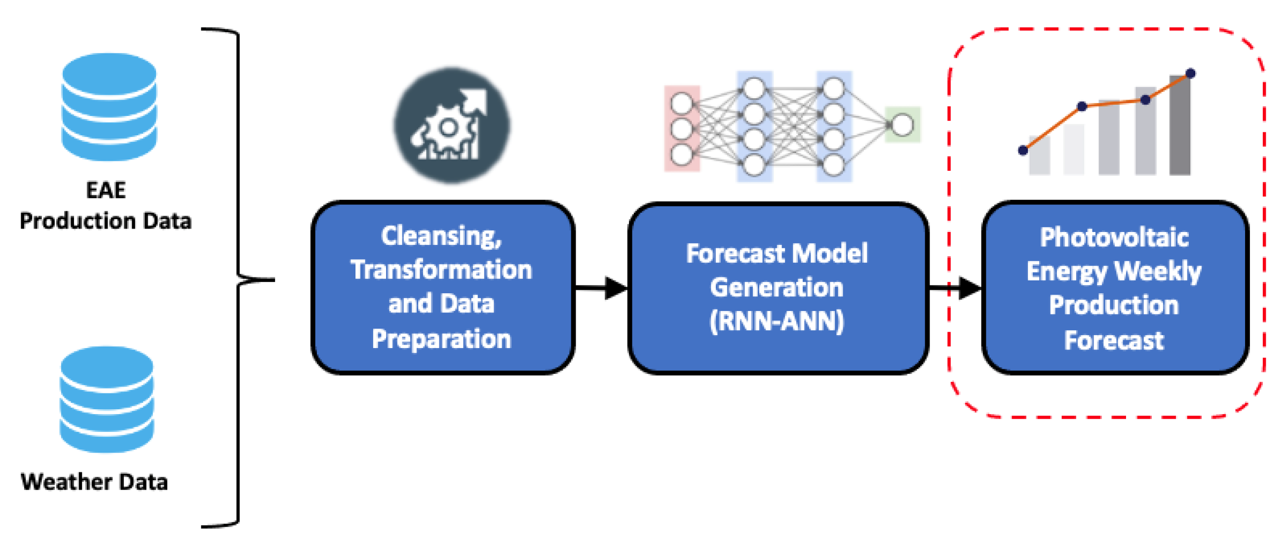
The main objective of the study is to generate models to forecast the photovoltaic energy weekly production of a solar plant with a high level of accuracy, based on historical production records and measurements of weather variables in a period of one year. Figure 5 illustrates the general work method used to achieve this objective.
As shown in
Figure 1, the data for this study comes from two sources: one providing EAE production records and the other providing weather variables collected from weather stations installed inside the solar plant. To achieve the study's objective, several operations must be performed on the data, such as integration, exploration, cleansing, filling and transformation.
Moreover, an appropriate data representation for handling time series with RNN techniques must be prepared. Afterwards, forecast models are generated using the RNN-ANN hybrid architecture with different hyperparameter configurations. The generated models are then trained, validated, and assessed using performance metrics. Finally, the models with the best performance and forecast results are selected, and the results are analyzed, interpreted, and compared.
3.3. Preliminary Analysis and Data Preparation
The dataset is stored in separate CSV files, with each file containing information for a single month of measurement. As a result, the frequency of the records varies. EAE measurements are taken hourly, while weather variables are measured every 5 minutes.
The daily EAE production is measured in kilowatt-hours (kWh), and the weather variables are as follows: compensated irradiation in watts per square meter (W/m²), ambient temperature in degrees Celsius (°C), wind speed in kilometers per hour (km/h), and wind angle in degrees (°). The data is accompanied by a timeline consisting of date and time.
To integrate data from both sources, an exploratory analysis was first carried out. It was observed that the values of the weather variables did not vary substantially within one hour. Therefore, it was decided to establish the average value of each weather variable for every hour, aligning them with the same hourly frequency as the records of the EAE variable.
The variables related to date and time are combined into a single column. However, solar radiation presents difficulties in the range of values due to negative values recorded by some pyranometers (solar radiation sensors) in the absence of solar radiation, when they should be zero. To address this issue, all negative solar radiation records are replaced with zeros. The data set also contains missing data in various segments, particularly in weather variables. To address this, various data filling techniques are applied, depending on the characteristics of the variables.
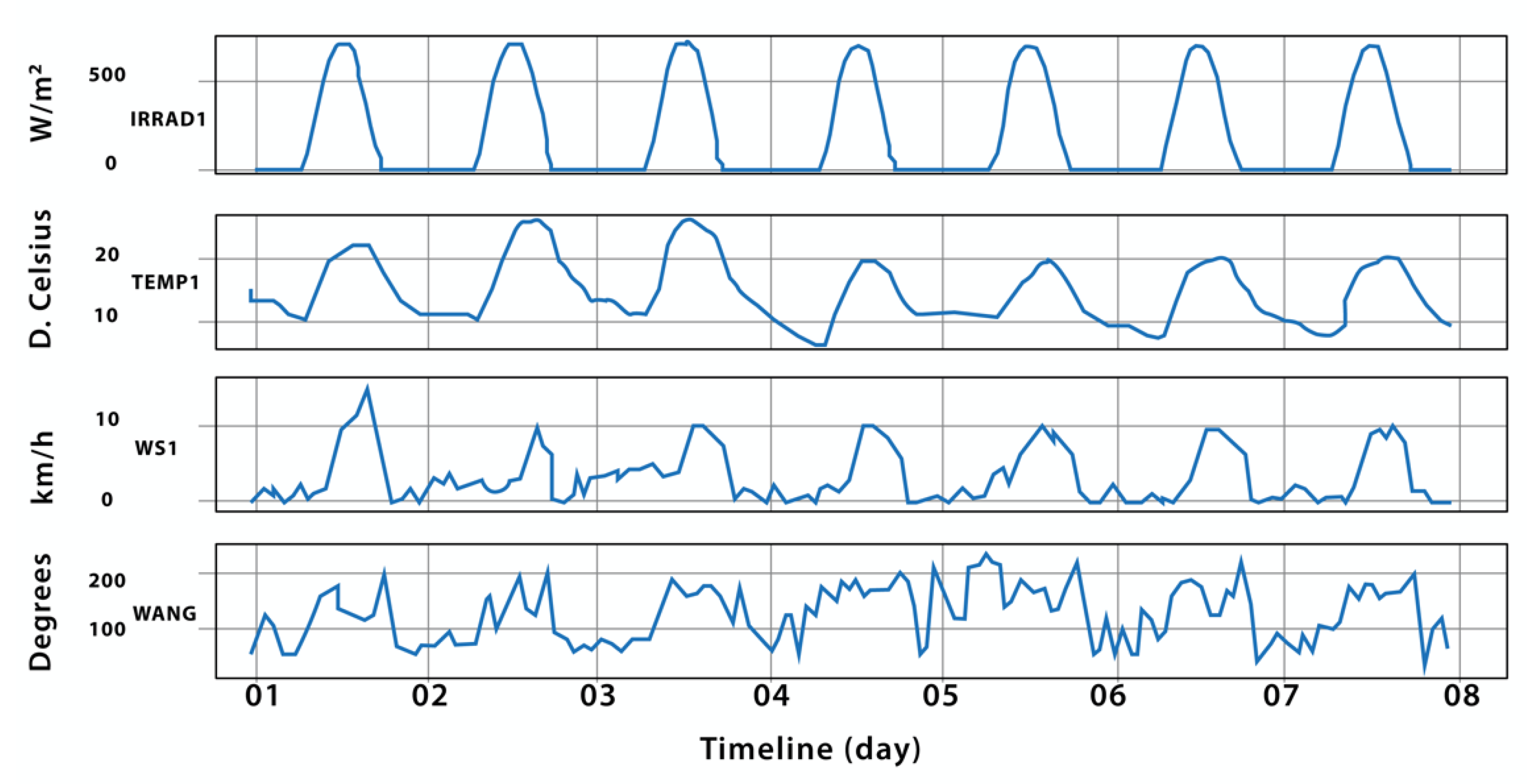
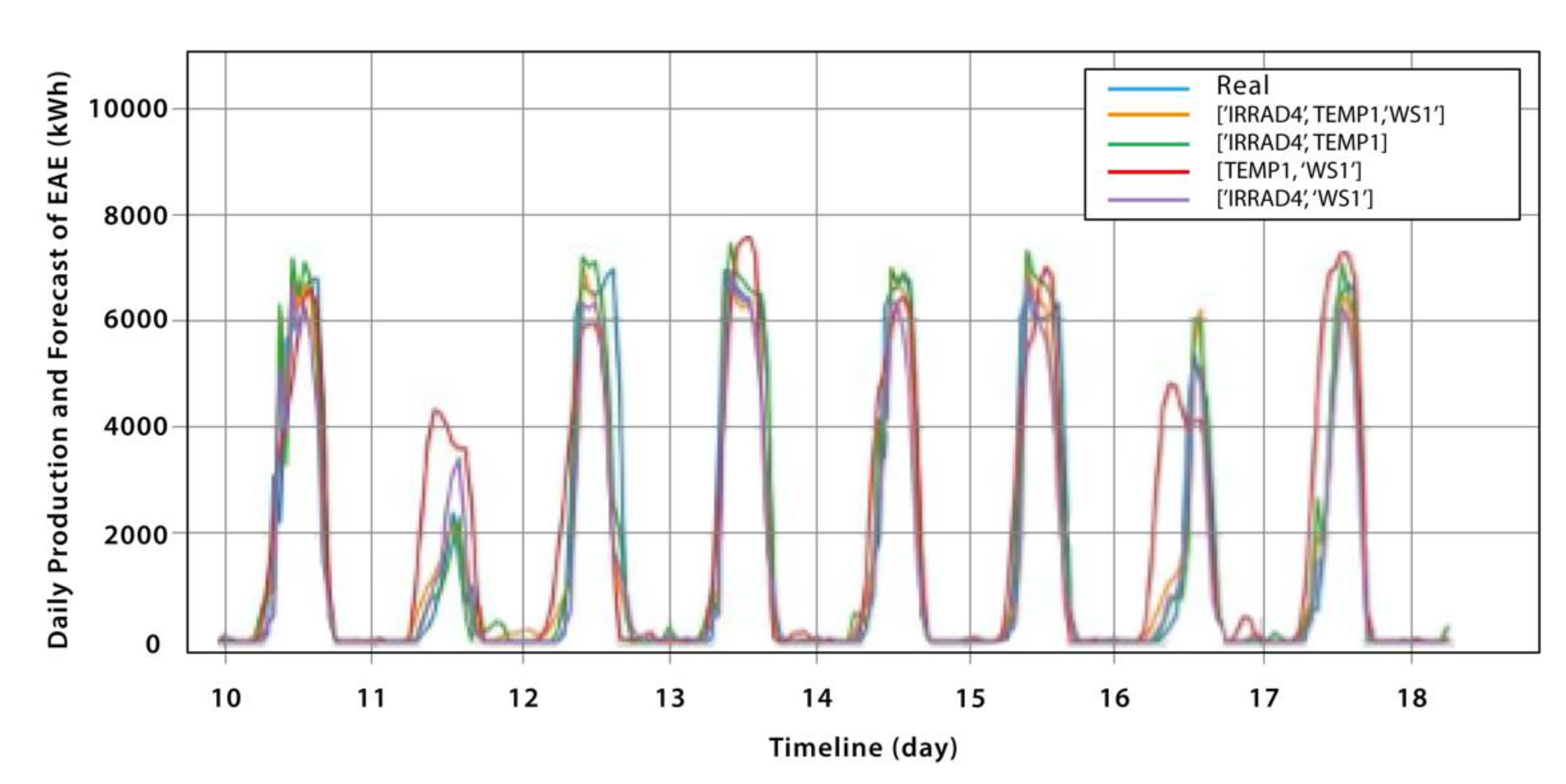
Figure 2 shows a representative sample of one week of weather variable records. It can be observed that temperature and solar radiation behave similarly, indicating a high correlation. However, wind speed and angle exhibit a chaotic and irregular pattern. As a result, missing values are handled differently for these variables. Specifically, missing values for wind speed and angle are filled using the previous value, considering that the curves of these variables show local trends, and each value is closely related to the previous one.
In the case of variable temperature and solar radiation, a method of filling in missing data based on the average is used. Each missing value is replaced by the average of the values of the seven days before or after, corresponding to the same time of day. For example, if the temperature value of June 14 at 10:25 a.m. is absent, the average of the temperature values at 10:25 a.m. of the seven days before is calculated, from June 7 until the 13th of the same month. The value resulting from this calculation is used to replace the missing data. This method respects the local and daily trend of the variables. It is valid and can be carried out since the missing data segments do not exceed 288 records. These methods are selected for their speed of execution and satisfactory results for relatively small missing segments.
On the other hand, the electrical variable EAE does not have the problem of missing values. However, it does present negative outliers in some records, which do not make sense in this type of data. It is inferred that this anomaly may be caused by the measuring instrument used to capture the record of this variable. To solve this, the negative values are replaced by their absolute value, taking into account that at the points where these anomalies occur, the magnitude agrees with the expected values of the measurement.
In the EAE variable, there are also extreme values, and to address these cases, an analysis is carried out to identify the limit threshold for the range of values of this variable. It is taken into consideration that the maximum power obtained in the solar plant is around 9 MW, and for this reason, the threshold is set at 10 MW. As these cases are very rare, the values that exceed 10 MW are replaced by the value corresponding to the first value belonging to the 0.99 quantile of all the records of the variable.
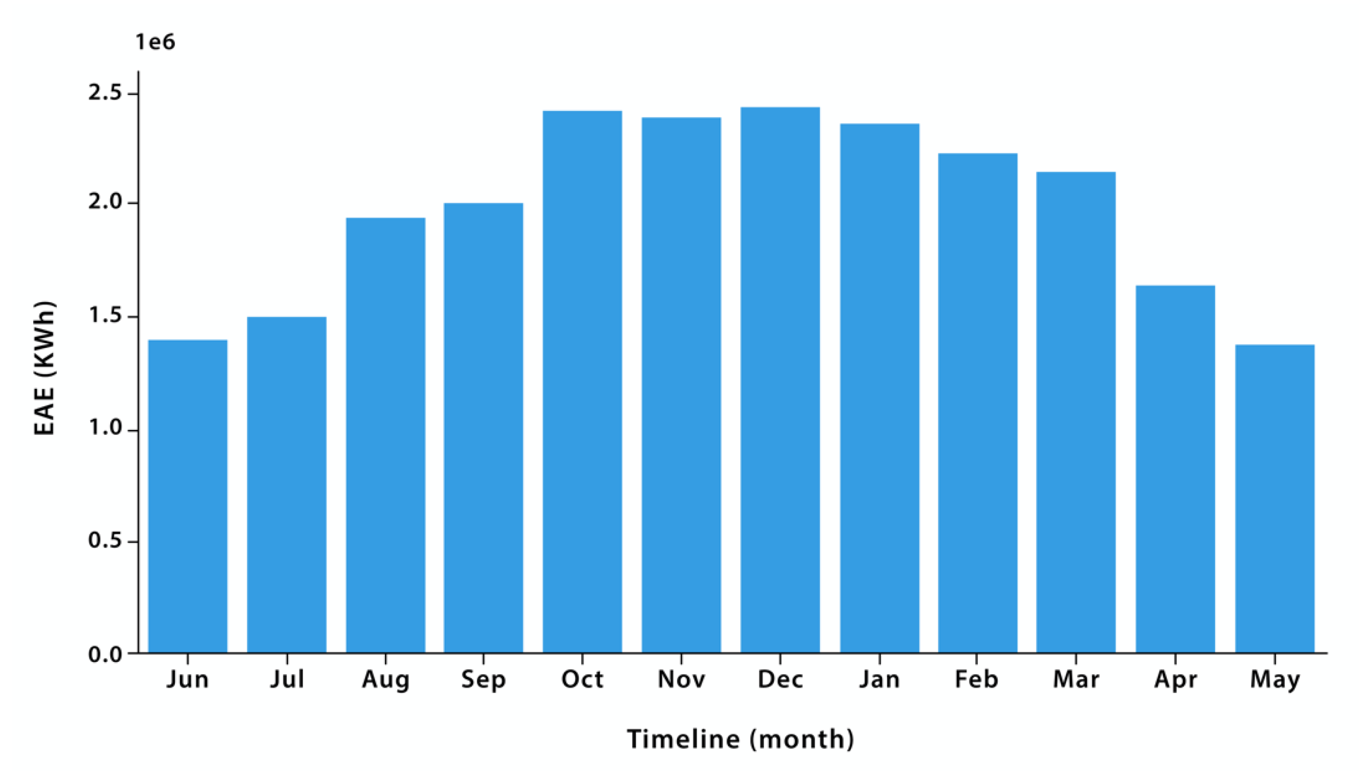
Additionally, the monthly generation of EAE of the solar plant during the observation period is analyzed, as shown in
Figure 3. It can be observed, the months of greatest production of photovoltaic energy and that go from October to March, must be Because in this area they correspond to the spring-summer seasons. The months of lower production are from April to September in the autumn-winter seasons. This is mainly due to the behavior of solar radiation in these stations, which is closely related to the EAE produced.
As mentioned above, the raw data is separated into different files per month, so a data integration task must be performed initially by processing each file. Then, preprocessing tasks are carried out for each variable. Once all the above steps are completed, the processed data is added to a single table that accumulates all the data for the work period in chronological order.
3.4. Data Transformation
Once the previous data preparation has been completed, ad-hoc transformations must be carried out to be use it appropriately by the RNN technique. These transformations should be based on the characteristics of the technique and the model to be obtained. Both the inputs and the structure of the model must be prepared, and the dataset should be divided before moving on to the modeling process.
For this particular work, it is necessary to transform the data into a supervised structure since RNN models require training that is defined by input and output labels. Furthermore, considering that the research data is accompanied by a time stamp and the research objective is to make time-based predictions.
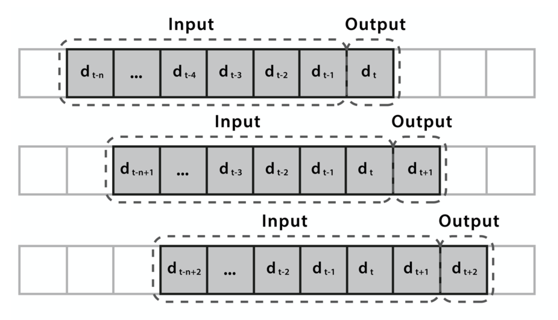
Based on the above, it is decided to define the inputs of the model as time series, which means that each input is composed of a sequence of
records. The models are trained by taking into account that for an output
, there is an input that covers several records from
to
. This transformation of the data is performed as many times as possible, considering the size of both the input and output sequences. Accordingly, the arrangement of the data is modified into input-output pairs, as shown in
Figure 4.
It is common for such transformations to undergo multiple changes during the data analysis process, typically due to modifications in the model or during the evaluation stage. These changes may often involve adjusting the sizes of the input and output sequences.
Finally, it is necessary to apply normalization to the data so that they can be re-scaled and managed within the same range, which allows minimizing the effect of variation or noise. One of the most commonly used types of normalization is the minimum-maximum normalization, which involves transforming each data point according to the following equation:
This process is carried out independently for each variable since they have their own range and scale. Once the model results are obtained, they must be inverted or denormalized to obtain the values in the original scale. For this work, standardization is used since it yields better results.
3.5. Model Generation Tool
A computational tool has been developed to automate the entire process, from data extraction and cleansing to data preparation and transformation, as well as the generation of forecasting models with their corresponding graphs, model training and validation, and performance evaluation using various metrics. This tool provides a general framework for carrying out time series forecasting tasks and can be adapted to different scenarios and data sources.
This tool is developed using the Python programming language and the TensorFlow framework, which has a comprehensive system of open-source tools, libraries, and resources that enable innovative machine learning. Additionally, the Keras API is used, which is one of the main components of TensorFlow and covers each step of the machine learning workflow.
As an input, the tool requires two files: one with the training and validation dataset and another with the configured hyperparameters. For each execution, the tool generates two output files. The first file contains the generated model and its graphs of loss, forecast, and dispersion function curves, comparing the forecast data with the actual data on the weekly production of EAE. The second file contains the results obtained for each of the metrics applied to the model.
This method of building the computational tool provides flexibility and generalization of the inputs. For example, it allows for the reconfiguration of hyperparameters to obtain a different model, changing the data set, or both inputs simultaneously.
5. Results and Discussion
Models were developed to accurately forecast weekly photovoltaic energy production based on historical EAE records and weather measurements, both of which were accompanied by a timeline. These models were developed with reference to various related works analyzed.
The main characteristic of the implemented RNN-ANN models, is that their architecture comprises a first hidden layer consisting of recurrent neurons with LSTM or GRU units, and a second hidden layer consisting of shallow MLP neurons.
There are several hyperparameters that need to be appropriately configured for the RNN-ANN forecasting model.
Various experiments are conducted from a base model to determine the appropriate hyperparameter configurations. The experimental part of the work focuses on generating two types of models based on the input variables.
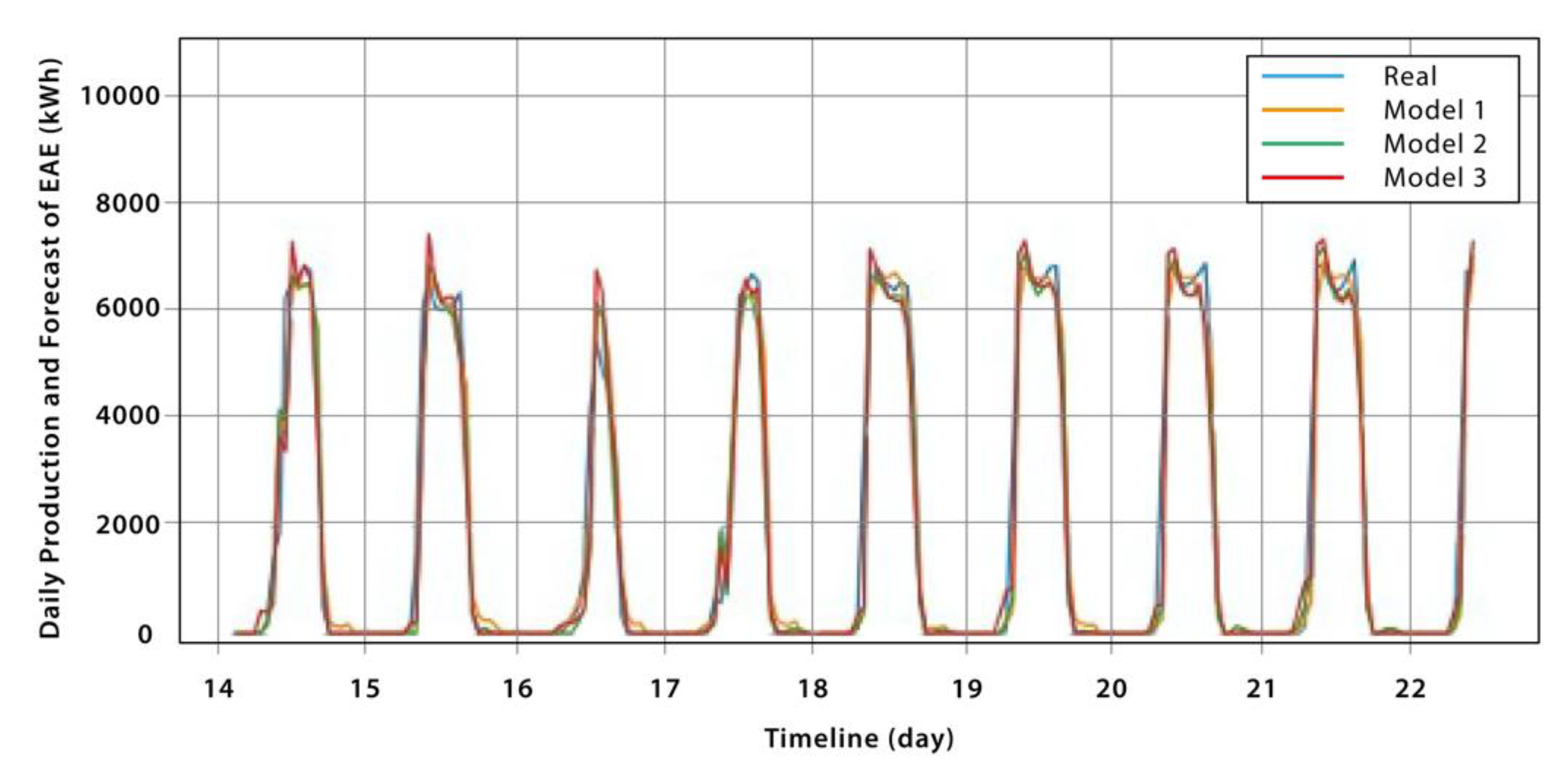
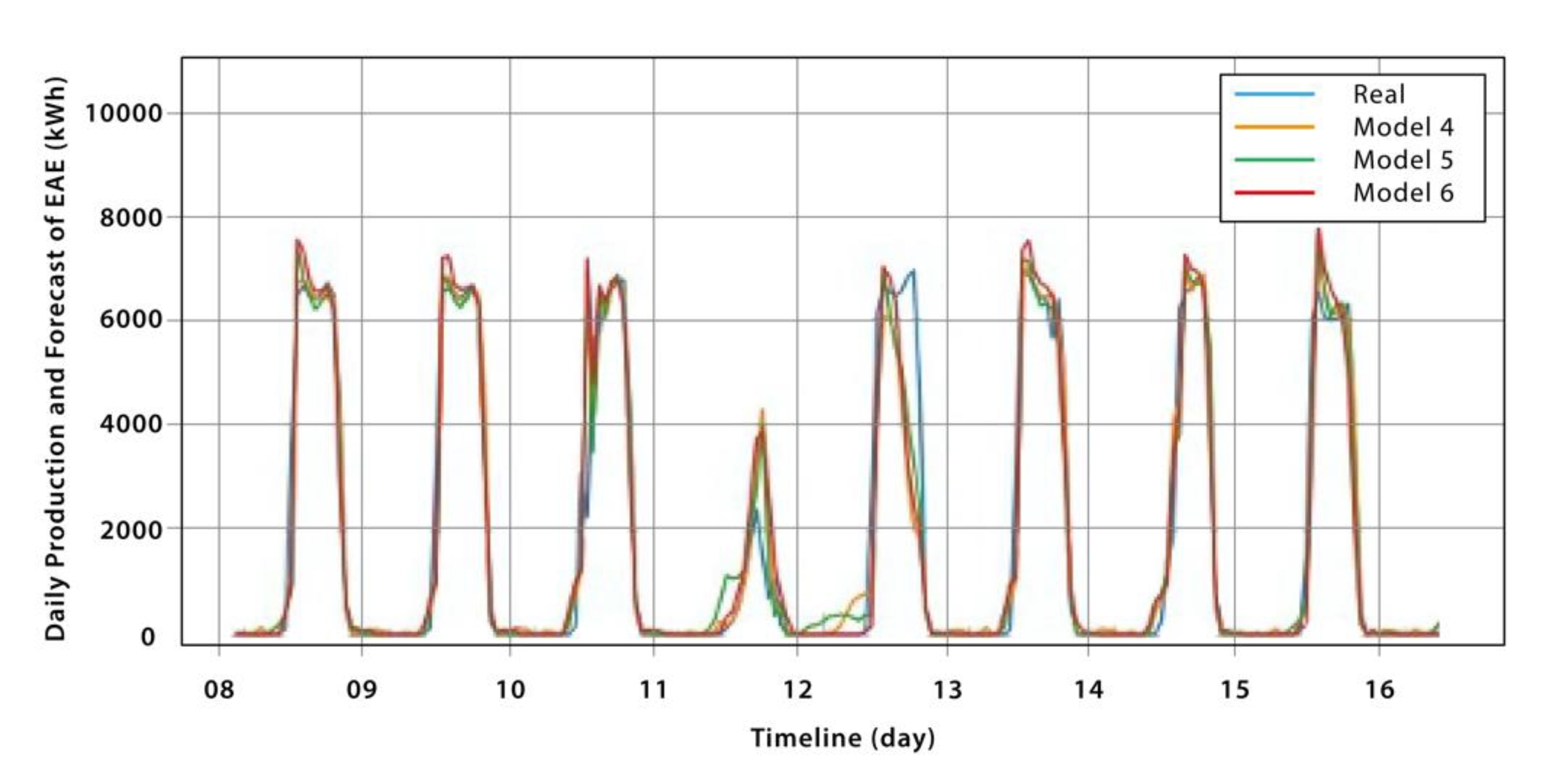
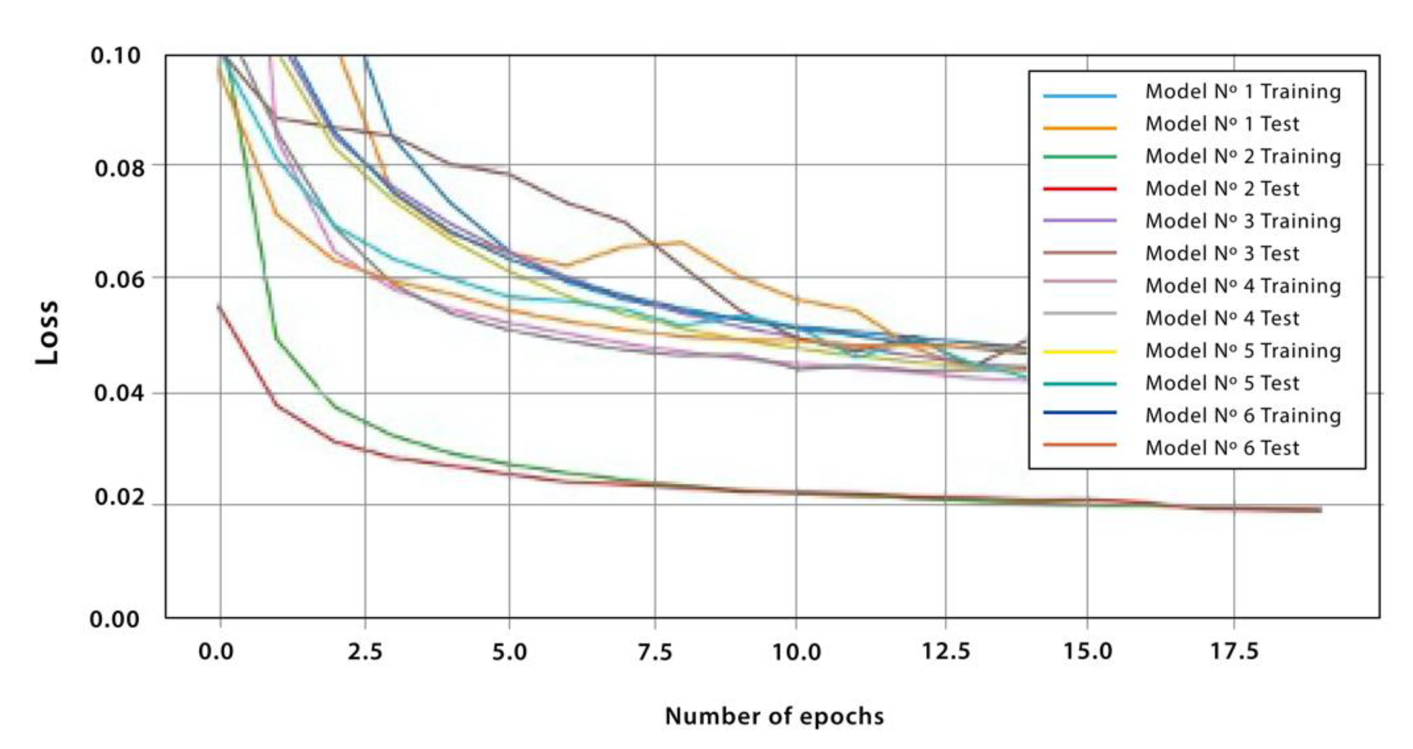
The first type of model utilizes the EAE variable along with the IRRAD, TEMP, and WS weather variables. It uses 20 recurrent neurons and divides the dataset into 90% for training and 10% for validation. The configurations can be seen in
Table 1 and
Table 2. Six models of this type are obtained, which yield good results in the evaluation metrics applied, as shown in
Table 3.
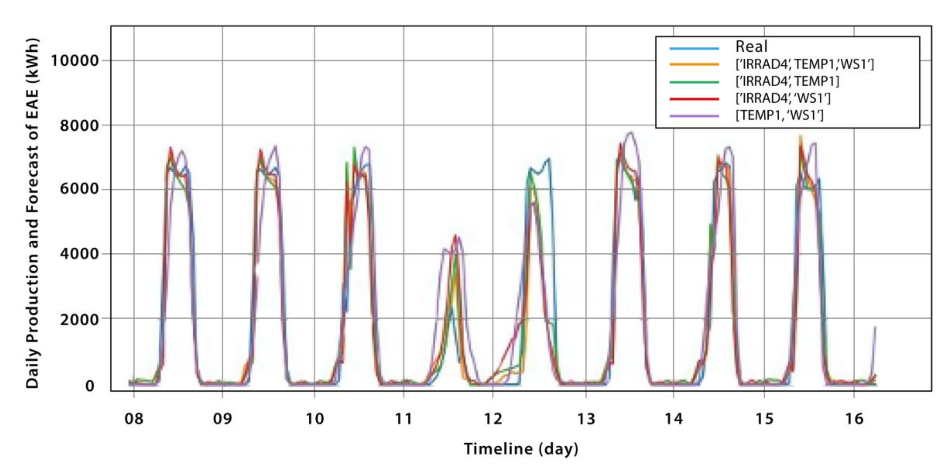
And for the second type of model, only weather variables are used and eight models are obtained with different combinations of these variables, differentiated only by the input sequence size. The hyperparameters used for these models include 20 recurrent neurons and a 90% training and 10% validation data set split, which can be seen in
Table 4,
Table 5 and
Table 6.
The models of the second type present lower values in their metrics compared to the models of the first type, which can be observed by comparing
Table 3,
Table 5 and
Table 6. This result is expected since the absence of the EAE variable as input makes the model more prone to issuing output distortions. However, these models have the advantage of being able to use information from a conventional weather forecast to predict the production of photovoltaic energy from a solar plant.
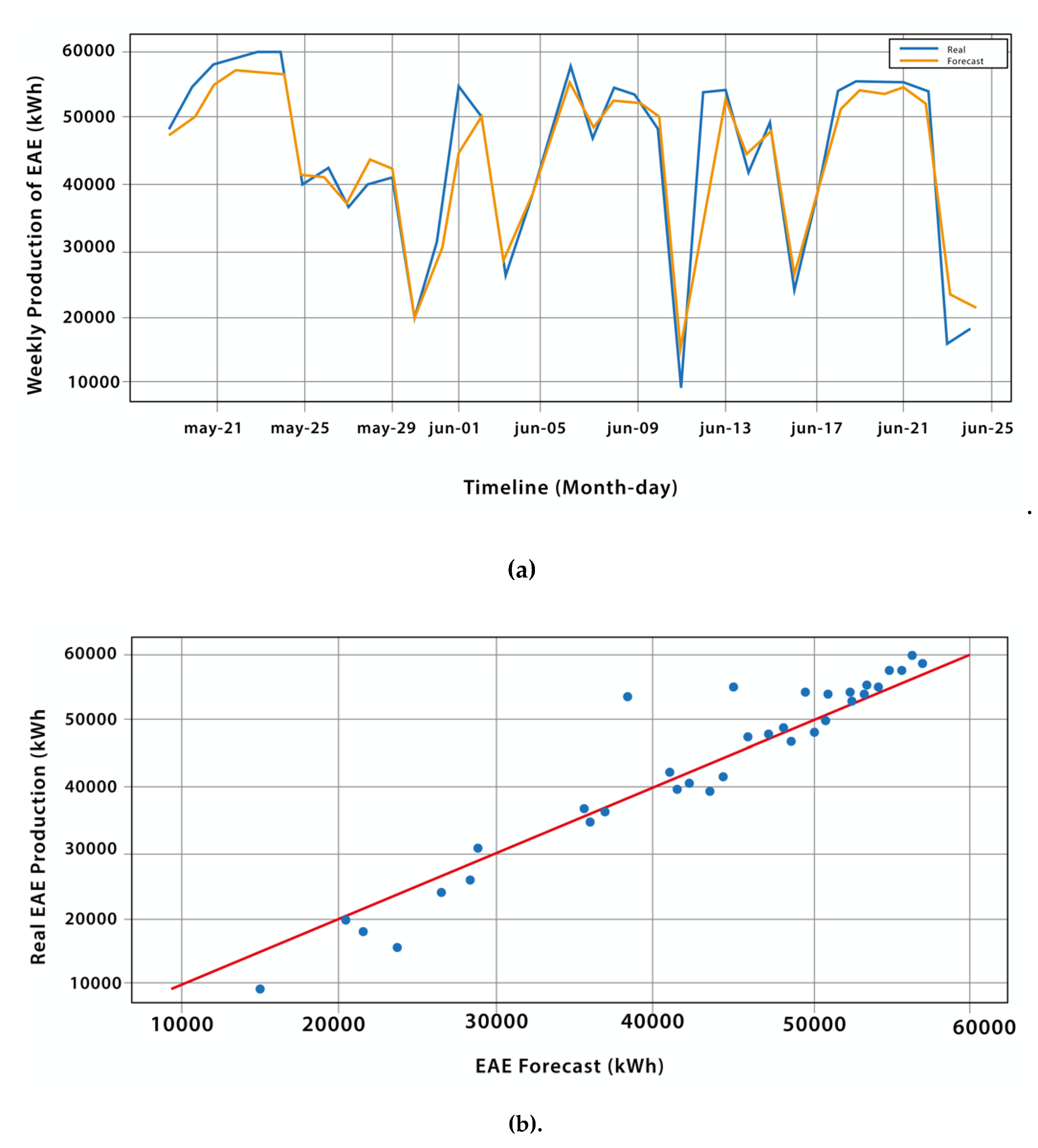
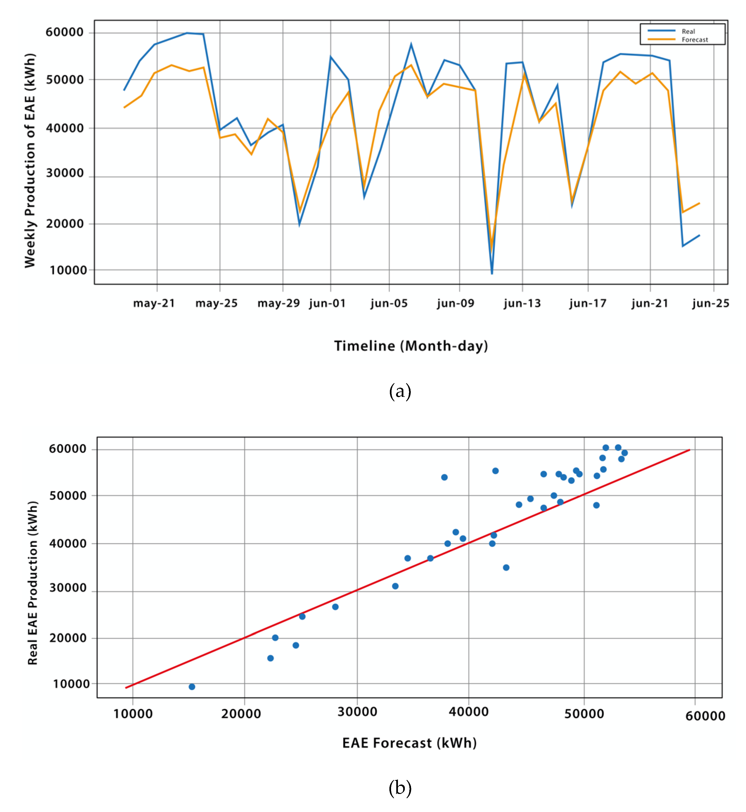
Table 7 shows the metrics of the best-performing models from each type. For the first type, Model 4 achieved the best results, while for the second type, is the model that forecast from the combination of the variables of solar radiation and temperature.
Although both models are capable of forecasting the weekly production of photovoltaic energy, they exhibit small errors and differences in some observed intervals. Nevertheless, these predictions can become more useful by increasing the volume of data and extending the forecast period.
Figure 10 and
Figure 11 illustrate some results of the chosen models, as indicated in
Table 7. In each figure, graph (a) displays the weekly forecast for the months of May and June, while graph (b) presents a scatter plot comparing the predicted values to the actual values of the solar plant's weekly EAE production.
It is observed that both models are able to accurately forecast the weekly production of photovoltaic energy, maintaining a similar behavior to the curve of real values. The scatter plots indicate a clear correlation between the predicted data and the actual data, although there are some points that are far from the ideal line, suggesting that further improvements can be made to the models.
Overall, it can be concluded that for weekly analysis, the models that incorporate the EAE variable provide better forecast results compared to the models that use only meteorological variables as input. This suggests that the EAE variable is a relevant factor to consider when predicting the production of photovoltaic energy.
6. Conclusions
With this study, it has been confirmed that the RNN-ANN hybrid architecture proposed in [
7] is capable of generating accurate models to forecast the weekly production of photovoltaic energy in a solar plant. This was achieved by considering various input variable combinations and hyperparameter configurations. The results demonstrate the potential of this approach to improve the accuracy of energy production forecasting, which is critical for the efficient management and planning of renewable energy systems.
The RNN-ANN hybrid architecture used differs from the approaches analyzed in this article, which also propose hybrid models. However, these models use other techniques in combination with ANNs, such as SVM or GA, and statistical models like Bayesian networks and ARIMA.
Another noteworthy contribution of this work is the diversity and quantity of models presented. It is important to note that two types of models were developed to forecast the weekly production of photovoltaic energy. The first type of model utilizes EAE records and weather variables as input variables, and 6 models of this type were evaluated, as shown in
Table 3. The second type of model uses only weather variables, and 8 models of this type were evaluated, as demonstrated in
Table 5 and
Table 6.
In relation to the results of the generated models, both types of models achieve good precision in forecasting the weekly production of photovoltaic energy, and the best performing model for each type is selected, as shown in
Table 7. Model 4 of the first type has an RMSE of 0.19, MSE of 0.03, MAE of 0.09, a correlation coefficient of 0.96 and a coefficient of determination of 0.93. The selected model of the second type, while presenting less precision in some metrics (RMSE = 0.24, MSE = 0.06, MAE = 0.10, Coef. Corr. = 0.95 and Coef. Det. = 0.90), still shows positive performance for making predictions.
Another characteristic that stands out in this research work, compared to others analyzed in section 2, is the large size of the dataset (more than 100,000 records) used for model training and validation. The dataset is made up of records for a whole year and with one-hour intervals, both of historical EAE production and weather variables. This was clearly one of the factors that contributed to the achievement of good forecast accuracy of the models obtained.
Another differentiating contribution of this research work is the development of a computational tool for implementing the hybrid architecture. The tool was developed using Python language, TensorFlow framework, and Keras API. Its main feature is its simplicity and flexibility in generating different forecast models. The encapsulation and generalization of the required hyperparameters, as well as the input data set, allow for the creation of a large number and variety of models. For each model, the tool generates separate files containing resulting graphs (prediction, loss function, prediction dispersion), as well as the results of all performance metrics.
The generality of this computational tool allows it to be applied in other contexts that require generating predictive models based on time series using RNNs. It would only be necessary to adjust the input data set by following the transformations described in subsection 3.4 of section 3, and to configure the required hyperparameters indicated in section 4 (Tables 1, 2, 4, 5 and 6).
It is important to mention that the accuracy of the models can be affected by different factors, both internal and external. Among the internal factors, one can consider the configuration of hyperparameters and the size of the dataset used for both training and validating the models. External factors are generally associated with physical aspects such as the composition of photovoltaic modules, failures in solar plant installations or photovoltaic panels, damages or mismatches in weather stations, among others.
The forecast models generated are useful tools for solar plants and their operators. Through the forecasts they provide, efficient planning can be carried out to achieve a balance between the generation capacity and consumption of photovoltaic energy. Improving the accuracy of the predictive models is essential to have a more reliable estimate of photovoltaic energy production, which can be added to existing electrical systems. These models can be validated using new data that represent different weather circumstances.
As future work, the following topics will be addressed:
Generation of models with other RNN configurations and new combinations of hyperparameters to achieve greater precision;
Increasing the sample dataset by incorporating new data records for the model training and validation processes;
Generating new models by integrating variables related to external factors or physical aspects such as elements of the internal composition of photovoltaic modules, temperature generated by solar radiation on these components, among other aspects;
Further research could explore the application of this approach to other renewable energy sources and the optimization of hyperparameters to improve model accuracy even further.
