Detecting Potential Outliers in Longitudinal Data with Time-Dependent Covariates

Preprint

Article

Detecting Potential Outliers in Longitudinal Data with Time-Dependent Covariates

Altmetrics

Downloads

240

Views

Comments

A peer-reviewed article of this preprint also exists.

Submitted:

05 May 2023

Posted:

06 May 2023

You are already at the latest version

Alerts

Abstract

Outliers can influence regression model parameters and change the direction of the estimated effect, over-estimating or under-estimating the strength of the association between a response variable and an exposure of interest. Identifying visit-level outliers from longitudinal data with continuous time-dependent covariates is important especially when the distribution of such variable is highly skewed at follow-up visits. The primary objective was to identify potential outliers at follow-up visits using interquartile range (IQR) statistic, motivated by a large TEDDY dietary longitudinal and time-to-event data with a continuous time varying vitamin B12 intake as the exposure of interest and time to developing Islet Autoimmunity (IA) as the response variable. The IQR method was also applied to simulated data. To assess the impact of IQR-method detected outliers, data was analyzed using Cox-proportional hazard model with robust sandwich estimator. Partial residual diagnostic plots were used to detect highly influential outliers. Results showed how some of the detected outliers had large influence on the Cox regression model and changed both the direction of hazard ratios and the strength of association with the risk of developing IA. In conclusion, the IQR method is useful in identifying potential outliers at visit-level which can be further investigated.

Keywords:

Subject: Public Health and Healthcare - Other

1. Introduction

In any statistical data analysis, analysts examine the data for unusual observations [1]. Outliers, also called extreme values, can be defined as observations that are unusually larger or smaller compared to other values in a data set [2]. Other studies have several ways of defining outliers such as being observations that deviate extensively from the overall pattern or expectation of the other data points (see [3,4]). [5] defined outliers as observations with large residual values or data values falling outside of an expected range [6]. These extreme values tend to skew the distribution of the data and may distort the model fit to the rest of the observations especially if they are highly influential.

Extreme values may be as a result of uncorrected data entry or system errors, self reporting bias or they can be genuine extreme values that are due to rare events. An outlier observation may have a large influence on the regression model parameter estimators that can change the direction of the effect, mask the effect, underestimate the effect, or overestimate the effect [7,8]. If extreme values are genuine (plausible) then, the fitted model that ignored the presence of outliers may not be a good fit and may lead to biased/misleading estimates.

Detection of outliers from longitudinal and time to event studies with continuous time-varying covariates pause a challenge in most applied research areas [9]. Although several methods to detect outliers have been employed in different study settings, most of them focus on detecting outliers after fitting regression models to simple data set. However, when the process of data management takes most of the time due to complexity of the datasets as is the case in dietary studies, conducting exploratory data analysis to detect these extreme values at the earlier stage can be extremely important. A more common process is using the knowledge and experience of investigators, using other published cross-sectional references or eye-balling using graphical outputs [10] to come up with single upper and/or lower values-cut-offs across the data set. These methods are arbitrary, lack clear justification and may vary from one study to another. The generated cut-offs cannot be generalized to other studies and may require more careful consideration when the data is longitudinal in design.

[11] used conditional growth percentiles to identify outliers in growth trajectory data and defined outliers to be observations 4 standard deviations (

σ

) away from the expected (conditional) value. However,

σ

and means (

μ

) are affected by extreme observations thus not suitable measures of spread and location, respectively, where the data is skewed [12]. Additionally, conditional growth percentiles method cannot be applied to a subject’s first measurement (visit).

Other studies have used robust regression methods to detect outliers on a longitudinal electronic health data records [13], whereas [14] calculated age and sex-adjusted height, weight and body mass index z-scores to identify extreme values for intra-individual trajectories. Also, [15] fitted non-linear mixed effects models enhanced with algorithms to detect outliers for longitudinal growth datasets.

By definition, a z-score for a particular observation x is the number of standard deviations that it falls away from the mean. That is,

z = \frac{x - \bar{x}}{s}

where s is the sample standard deviation and

\bar{x}

is the sample mean. The use of z-score statistic requires the assumption that the data has a bell-shaped distribution. In that case, it is expected that

\approx 68 %

of the data will have a z-score of

\pm 1

\approx 95 %

of the data will have a z-score of

\pm 2

and

\approx 99.7 %

of the observations will have a z-score of

\pm 3

which is the empirical rule for any normally distributed data. A z-score

≊ 0

indicates that the data point is located at or near the mean of the dataset, and, a larger (positive or negative) z-score indicates that the data point is larger than or smaller than almost all other observations in the data [2]. This method is not appropriate for highly skewed variables. Other studies used jackknife residuals and defined an outlier with a cut-off of

\pm 5

in their longitudinal childhood growth data [16]. Studentized residuals have been used by [17] with a cut-off of

> 2 σ

to define outliers whereas [18] used a cut-off of

\pm 6

for a longitudinal study on obesity prevalence and weight change in children and adolescents together with cross-sectional z-scores thresholds as defined by Centers for Disease Control.

Interquartile range (IQR) and median absolute deviation (MAD) statistics are simple and useful non-parametric methods that can be applied to detect potential outliers during the exploratory data analysis stage. MAD method has been used to detect and remove outliers by several studies (see [5,12,19,20]). For a given data set

x_{1}, x_{2}, \dots, x_{n}

, MAD is defined as:

M A D = b \times (m e d i a n {| x_{i} - \hat{x} |})

where b is a constant (usually

1.4826

for a

N (μ, σ^{2})

variable),

\hat{x}

= median(x),

| x_{i} - \hat{x} |

is absolute deviation from the median and

m e d i a n {| x_{i} - \hat{x} |}

= median of these absolute deviations.

To declare

x_{i}

an outlier, a MAD rejection criteria is given by the following expression [21]:

\begin{matrix} \hat{x} - k \times M A D < x_{i} < \hat{x} + k \times M A D \\ o r \frac{(x_{i} - \hat{x})}{M A D} > | \pm k | o r \frac{| (x_{i} - \hat{x}) |}{M A D} > k \end{matrix}

where

k > 0

is a scale factor.

Both IQR and MAD statistics are robust measures of dispersion that are more resilient to outliers than standard deviation. Means and standard deviations should not be used as a measure of location and spread, respectively, if the distribution is highly asymmetric.

Numerical IQR method and graphical assessment using box plots were described to be methods that successfully identified potential outliers in an educational achievement study to improve student learning [22]. Also, [23] calculated weight for length percentiles and then used the interquartile range method to detect and remove outliers in a longitudinal childhood genome study.

The IQR method is based on quartiles which are values that partition the data into four equal parts, each containing

25 %

of the observations. The lower quartile (

Q_{1}

) is the

25 t h

percentile, the middle quartile (

Q_{2}

) is the median (m) or the

50 t h

percentile, and the upper quartile (

Q_{3}

) is the

75 t h

percentile. Interquartile range (

I Q R

) measures the distance (spread) between the lower and the upper quartiles, that is

I Q R = Q_{3} - Q_{1}

. Graphical assessment of potential outliers using box plots is based on the interquartile range of a data set. This method measures the central half of the data for any shape of the distribution. It is a great alternative measure of dispersion that does not require symmetry and has no distribution assumptions since it uses percentiles and hence robust to presence of outliers.

The robustness of IQR and MAD has been shown by [24] that if

T_{n}

is a statistic on an ordered sample of size n, then,

T_{n}

has breakdown value b,

0 \leq b \leq 1

, if for every

ϵ > 0

{lim}_{X ({(1 - b) n}) \to \infty} T_{n} < \infty

and

{lim}_{X ({(1 - (b + ϵ)) n}) \to \infty} T_{n} = \infty .

The sample median (m) remains unchanged in the presence of extreme low or high values. If less than

50 %

of the sample

\to \infty

, then m and MAD will remain the same. If more than

50 %

of the sample

\to \infty

, then

m \to \infty

and so does MAD. The median in that case will be located within the outliers. As such, MAD has a breakdown value of

50 %

. Similarly, IQR has a breakdown value of

25 %

, breaking down when

Q_{1}

is located within the outliers [25].

The aim of this study was to describe how to identify potential outliers at follow-up visits using a non-parametric interquartile range (IQR) statistic method with its applications to real and simulated data. This ideas was motivated by a large TEDDY dietary longitudinal and time-to-event data set that had continuous time varying covariates as the main exposures of interest and time to developing Islet Autoimmunity (IA) as the response variable. Exploratory data analysis is illustrated based on simulated longitudinal data with and without extreme observations. We also show the impact of the IQR-method detected outliers using TEDDY dietary data. Methods details and results are provided in Section 2 and Section 3.

2. Materials and Methods

We describe the IQR method with application to data in the following sections.

2.1. Interquartile Range Algorithm

For each continuous time-dependent covariate of interest, do the following e.g. by country and (or) age (follow-up visit):

(i): Calculate $I Q R = Q_{3} - Q_{1}$ .
(ii): Define lower and upper limits of outliers as $[Q_{1} - k \times I Q R, Q_{3} + k \times I Q R]$ where $k > 0$ is a scale factor.
(iii): Flag observations outside these limits as potential outliers.

IQR lower-limits below zero were set to zero because food intake cannot be negative.

By default, graphical exploration of data using box-plots method use

k = 1.5

for detecting mild-outliers and

k = 3

for extreme-outliers limits. In our study, since the data is highly skewed and varies by country and age at follow-up visit, we experiment with varying values of k.

2.2. Choosing a Scale Factor (k) for Spread

The rationale for choosing k is to determine how far away from the median 50% of the data you would like to keep and define the limits of spread to be included for analysis. Three guidelines are provided below:

(i): k can be chosen arbitrarily. In this study, we explore $3 \leq k \leq 10$ .
(ii): k can be decided based on what percentage of data the investigator is willing to drop and not lose power for the statistical analysis.
(iii): k can be based on known distribution parameters. For instance, assuming the data follow a Gaussian distribution, the mean ( $μ$ ) is approximately equal to the median, and we expect that $\approx 68 %$ of the data lies within $μ \pm 1 σ$ , $\approx 95 %$ of the data lies within $μ \pm 2 σ$ , and $\approx 99.7 %$ of the data lies within $μ \pm 3 σ .$ An IQR encloses $50 %$ and $I Q R / 2 = 0.675 σ$ . An observation $x_{i}$ such that $3 σ < x_{i} < - 3 σ$ away from the mean may be defined as a potential outlier.

The extent to which a scaling factor k from the IQR method may be related with

σ

is illustrated below: for

k = 1.5

\begin{matrix} L o w e r l i m i t & = & Q_{1} - 1.5 (I Q R) = Q_{1} - 1.5 (Q_{3} - Q_{1}) \\ = & - 0.675 σ - 1.5 (0.675 - [- 0.675]) σ \\ = & - 0.675 σ - 1.5 \times 1.35 σ = - 2.7 σ \\ U p p e r l i m i t & = & Q_{3} + 1.5 (I Q R) = 2.7 σ \end{matrix}

Similarly, a

k = 1.7

has limits

[- 3, 3] σ,

and a

k = 3

has limits

[- 4.7, 4.7] σ

. For

k = 4

, the limits are

[- 6.1, 6.1] σ

, and a

k = 5

has limits

[- 7.4, 7.4] σ

2.3. Simulated Data

Two longitudinal datasets were generated to illustrate the IQR method’s ability to detect outliers at the exploratory data analysis stage. The initial data (data 1) was simulated with

n = 10, 000

subjects that were randomly assigned with 6 to 10 follow-up visits and a total of

79, 951

observations. The measured weight (kg)

y_{i j}

of subject i at visit j, for

j = 6, 7, 8, \dots, 15

years of age, was based on a linear random-coefficient model:

\begin{matrix} y_{i j} & = & 2 + 5.6 * a g e_{i j} + μ_{0 i} + a g e_{i j} * μ_{1 i} + e_{i j} \\ = & 2 + (5.6 + μ_{1 i}) * a g e_{i j} + μ_{0 i} + e_{i j} \\ = & (2 + μ_{0 i}) + (5.6 + μ_{1 i}) * a g e_{i j} + e_{i j} \end{matrix}

where the random intercept for subject i is

μ_{0 i .} \sim N (0, 3)

, random slope

μ_{1 i .} \sim N (0, 1)

and the random error

e_{i j} \sim N (0, 2) .

The second simulated data (data 2) was created by introducing eight extreme observations into data 1. In this setting, 4 subjects and 8 visits were randomly selected. The means

μ_{j}

and standard deviations

σ_{j}

of weight

y_{i j}

from each visit (visit j) were computed. Each of the 4 subjects were assigned arbitrary number of visits in which the new weights (kg) were re-computed to be d standard deviations away from the mean, expressed as

μ_{j} \pm (d * σ_{j})

, for

d = 5, 6, 7, 8, 10

where

μ_{j}

and

σ_{j}

are the specific means and standard deviations at visit j. The values of d were chosen based on the description provided in Section 2.2. For instance,

5 σ

away from the mean is equivalent to using a

k = 3

scale factor under the IQR method.

2.4. Motivating TEDDY Dietary Data

The real data that motivated this study was a longitudinal and time-to-event data set with time varying covariates. Dietary intake data was obtained from The Environmental Determinants of Diabetes in the Young (TEDDY), which is an observational longitudinal study that investigates factors associated with Diabetes (T1D) in children [26,27].

Full data set was obtained after undergoing cleaning and quality checks to remove obvious unexpected observations. The data had

94, 352

records from

8, 676

children followed from birth up to 15 years of age. Censoring was done at 10 years of age for this analysis. Diet was assessed by 24-hour dietary recall at the age of 3 months, by 3-day food record at the age of 6, 9, and 12 months and every 6 months thereafter until the subject developed islet autoimmunity (IA) or was censored at the end of the study period. Data was organized using the counting process. For the purpose of illustrating the IQR method, focus was on exposure to daily intake of vitamin B

_{12}

(µg/day), including intake from foods and dietary supplements [28] and the risk of developing IA. The Cox-proportional hazard model was used for analysis with robust sandwich estimator for calculating standard errors. All statistical models were adjusted for sex, Human Leukocyte Antigen (HLA) genotype DR3/4 status, family T1D status (FDR) and country. Vitamin B

_{12}

was treated as a continuous time dependent covariate.

A detailed illustration of the IQR method is provided with application to this data both at the exploratory stage before fitting time-to-event survival models and after, where residual diagnostics were assessed for highly influential observations.

2.5. Detecting Highly Influential Observations Using Residual Diagnostics

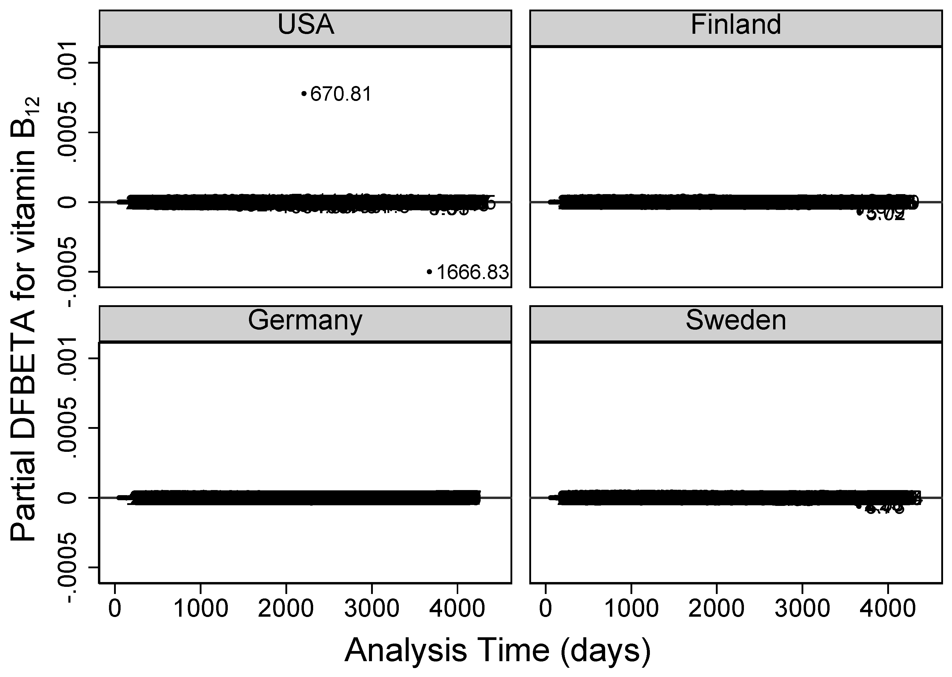
Residual diagnostics plots were obtained after fitting Cox regression models on the full TEDDY dietary data to further ascertain the influence of highly influential observations on the estimated parameters. Partial DFBETA measure of influence for vitamin B

_{12}

was plotted against analysis time and partial efficient score residuals were also plotted against analysis time. Partial residuals were calculated for each observation within subject. They are the additive contributions to a subject’s overall residual (see [29,30] for details). The partial DFBETA value estimates the change in the regressor’s coefficient due to deletion of that individual record.

2.6. Handling Detected Potential Outliers

Detected potential outliers by IQR method and diagnostic plots were handled as shown below:

(i): Naively ignored the presence of outliers for sensitivity analysis and fit standard Cox models to the whole data set.
(ii): The variable was log-transformed to base 2.
(iii): Detected outliers were inversely weighted so that they can lie within the lower and upper bounds using the following procedure: For each $x_{i}$ value that is outside the limits, compute weight

$w_{i} = m a x (| x_{i} - u p p e r_l i m i t |, | x_{i} - l o w e r_l i m i t |)$

Calculate a pseudo value $x_{j} = \frac{x_{i}}{w_{i}} + l o w e r_l i m i t$ . This method replaces the $x_{i}$ outlier value with $x_{j}$ that is bounded within the limits.
(iv): Dropped outliers based on IQR scale factors $k = 3, 5, 7, 10$ .

Statistical analysis was conducted using SAS

^{®}

Software version 9.4 [31], R Core Team (2023) version 4.3.0 [32] and Stata statistical software (release 18) [33].

3. Results

3.1. Results Based on Simulated Data

Table 1 shows summary statistics based on IQR method with a scale factor

k = 3

from the simulated data without outliers (data 1) and also shows the eight identified outliers from data 2 (data with outliers). There were no detected outliers from data 1 as expected since the data were simulated without extreme values. A

100 %

of all weights were within the expected lower and upper boundaries.

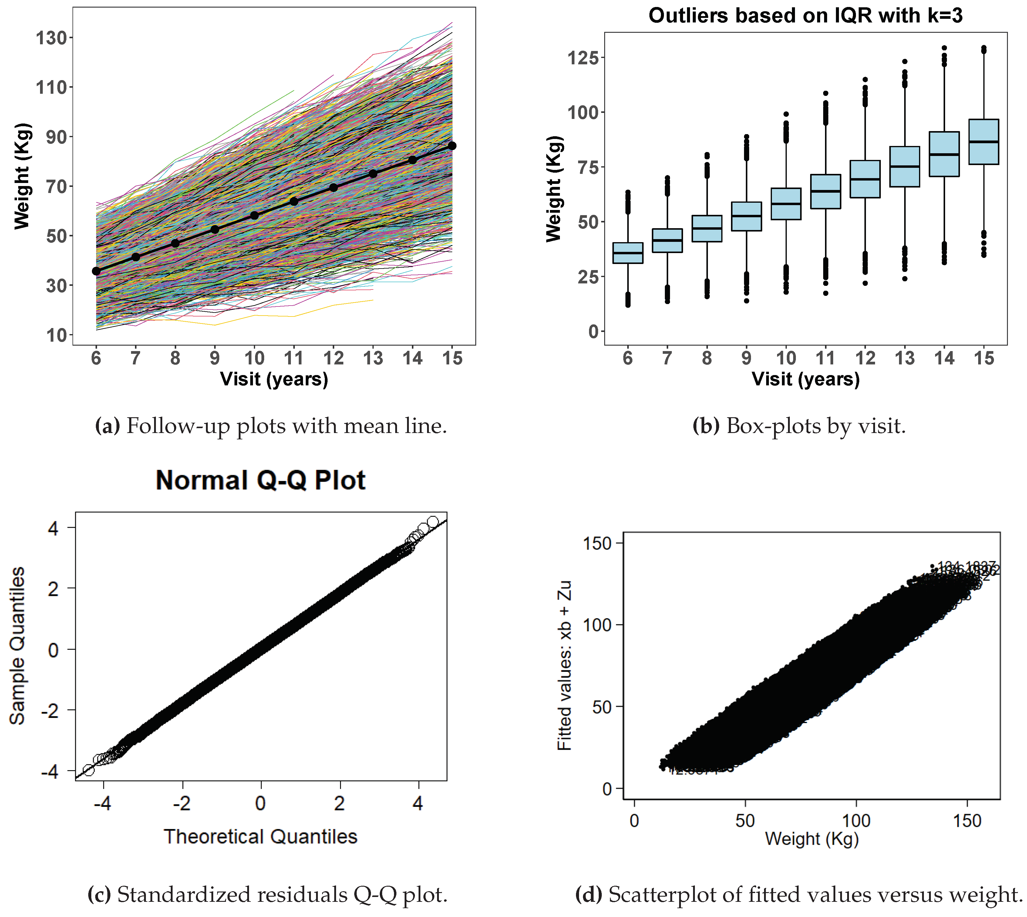
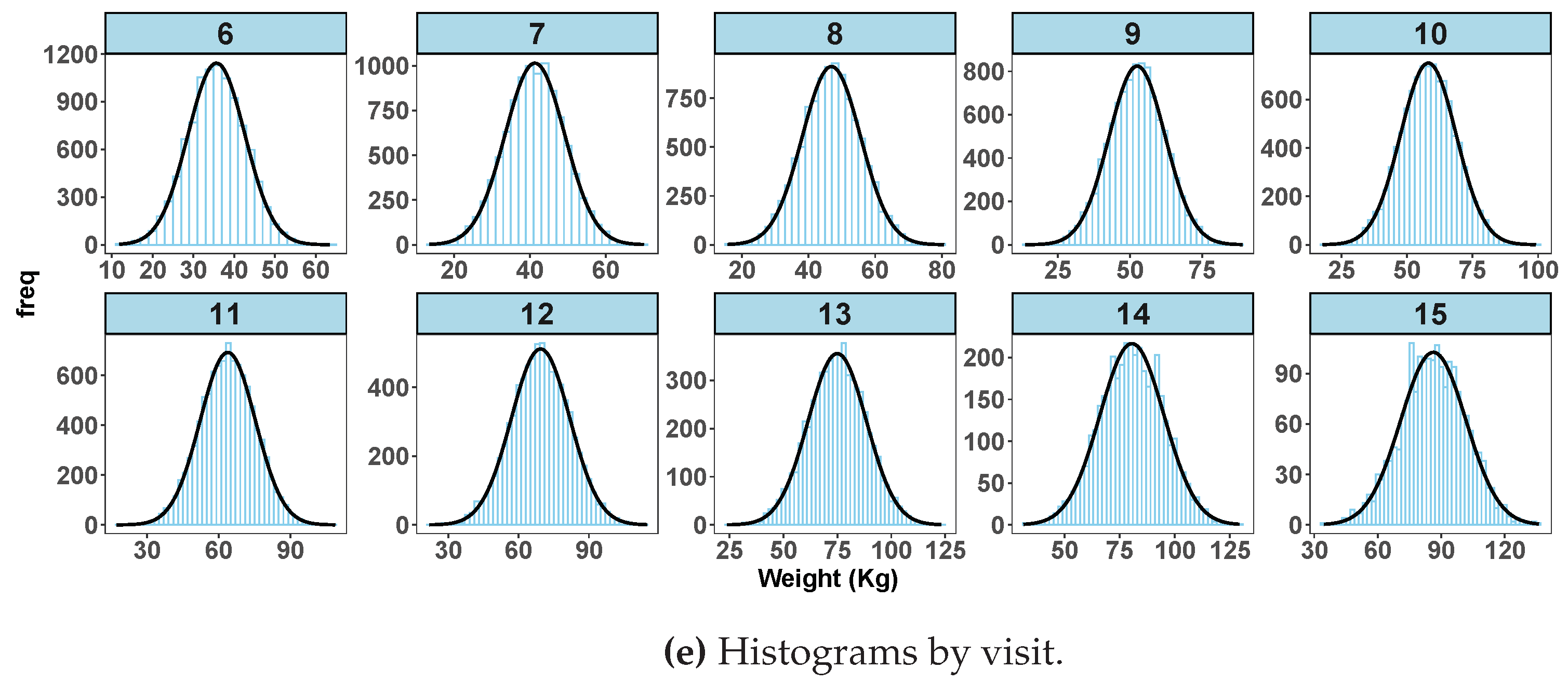
Figure 1 displays exploratory data analysis from simulated data with no extreme data points with spaghetti plot (Figure 1a), box plots (Figure 1b), normal quantile-quantile plots of standardized residuals (Figure 1c) and a scatter plot of fitted values versus observed weight (Figure 1d) after fitting a random coefficient mixed effect model. Histograms shown in Figure 1e are by age in years at visit. The box plot for

k = 3

does not show any indication of extreme values and neither are the histogram distributions.

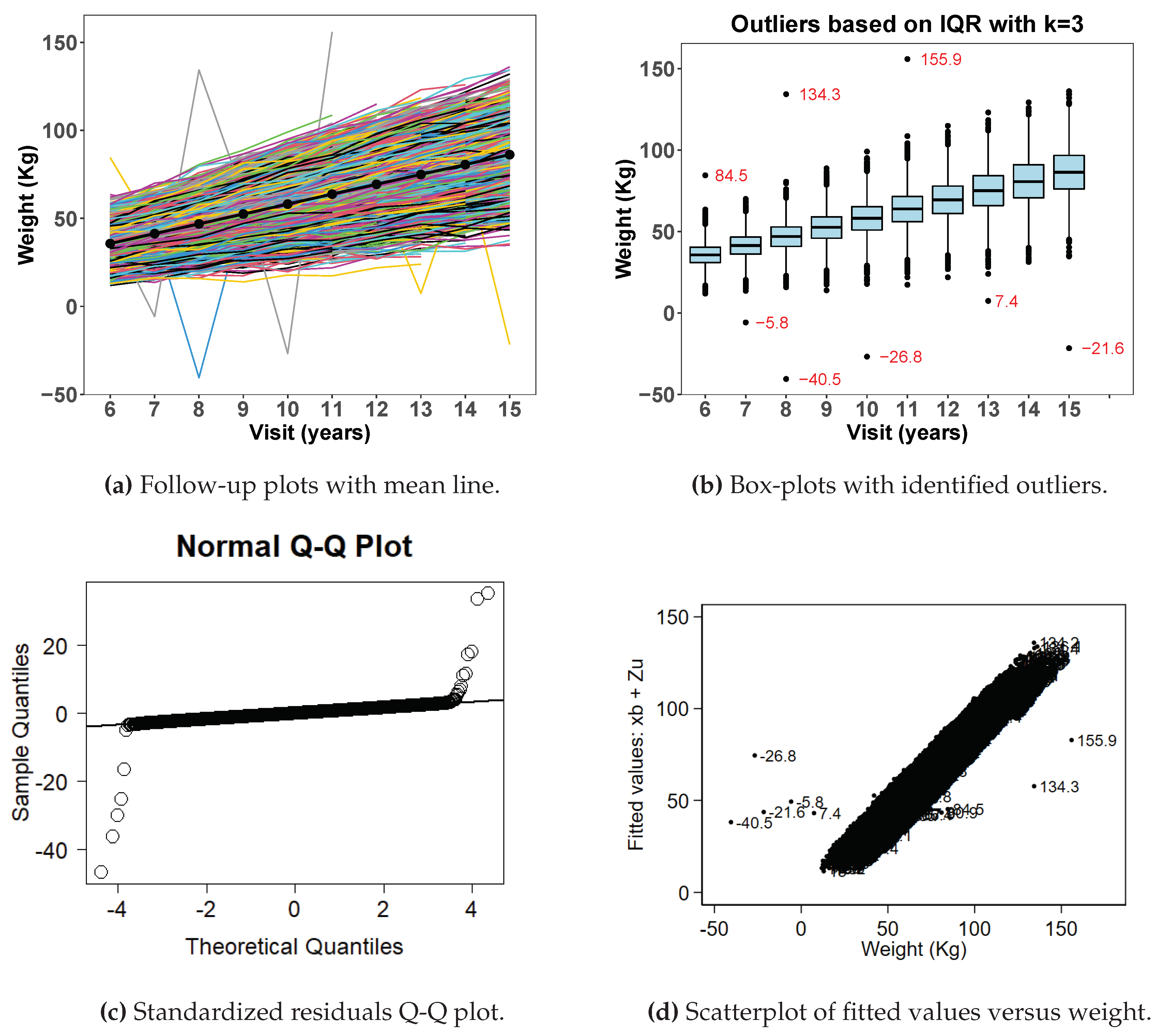
Figure 2 shows exploratory data analysis from simulated data with outliers. Figure 2a shows a spaghetti plot with extreme observations deviating from the rest of the data points. Similarly Figure 2b shows box plots with highlighted extreme observations by age at visit. Figure 2c shows normal quantile-quantile plots of standardized residuals and Figure 2d shows a scatter plot of fitted values versus observed weight after fitting a random-coefficient mixed effect model on the data. 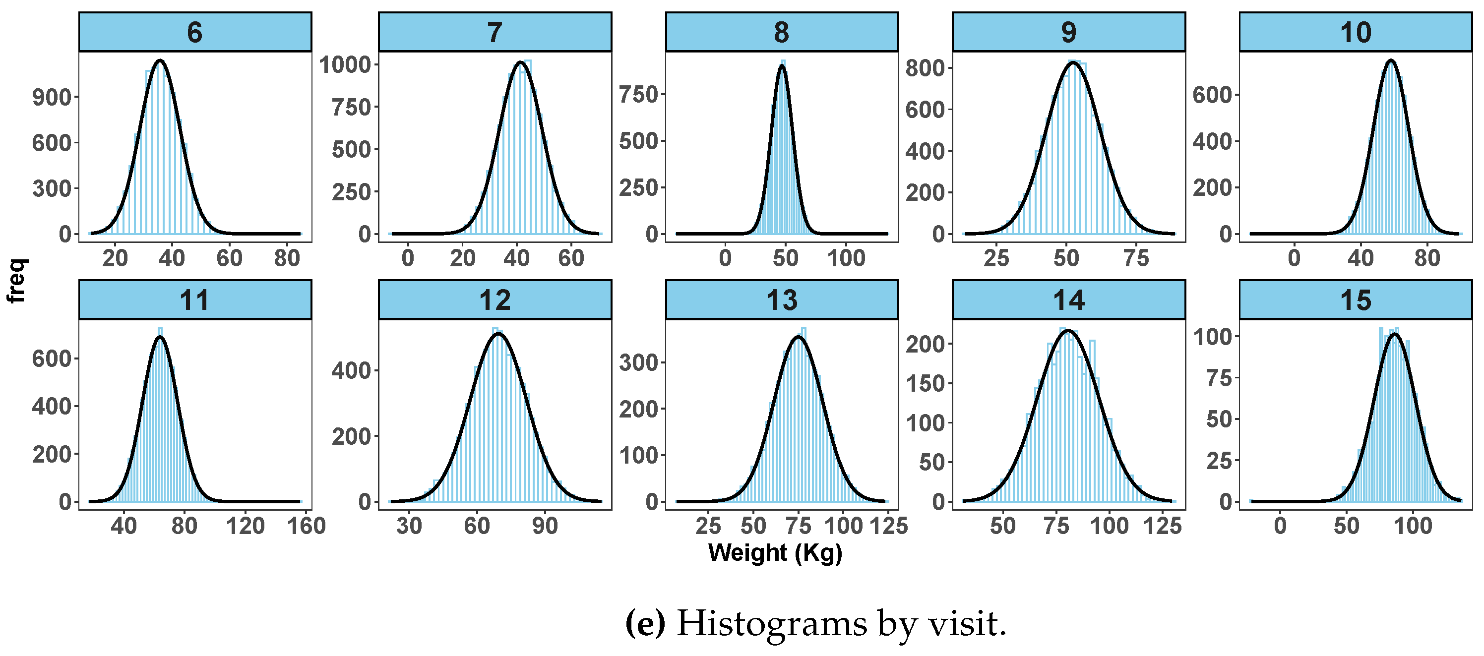Both figures (Figure 2c,d) show clearly that some observations are unusually larger or smaller than the rest of the data points. The visit-level histograms (Figure 2e) depict some skewness at some of the follow-up visits.

3.2. Results Based on TEDDY Dietary Data

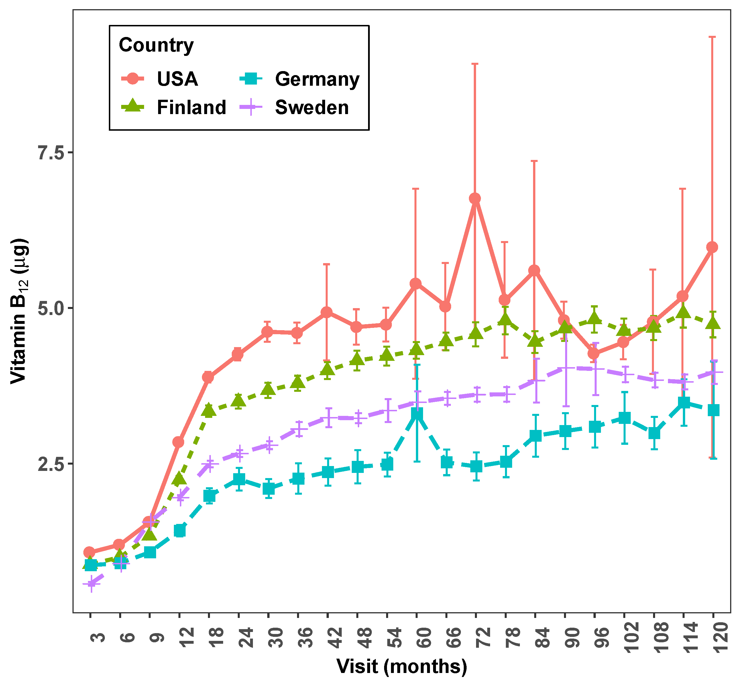
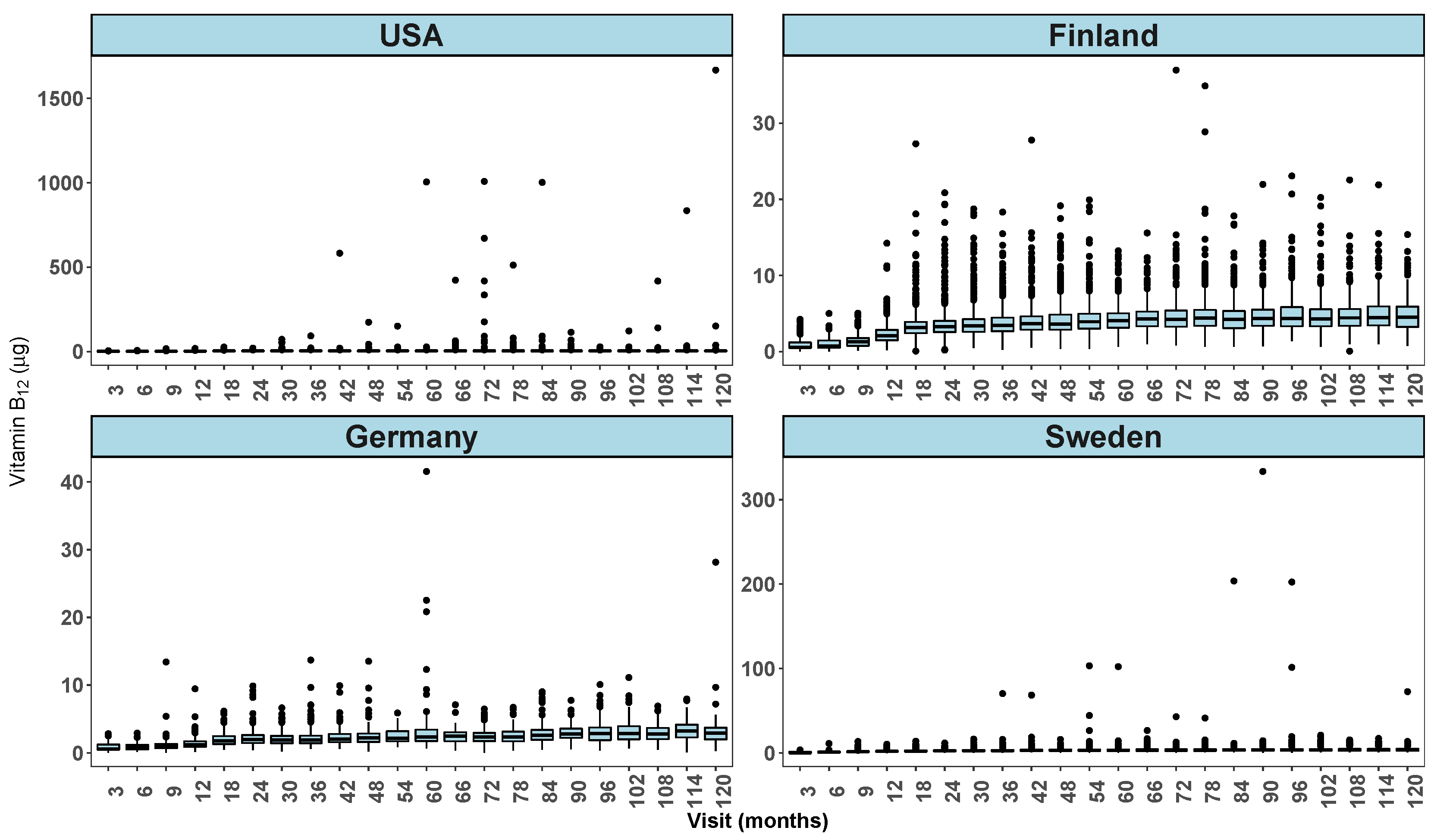
Country by visit exploratory graphs from full TEDDY dietary data are shown in Figure 3 and Figure 4. The line graph (Figure 3) shows how intake/day of vitamin

B_{12}

varies on average between countries and by visit. The box plot (Figure 4) shows the presence of several extreme values at some of the follow-up visits especially in the USA but also in other countries.

Table 2 shows hazard ratios (HR),

95 % C I

and P-values for analyses from fitted Cox-regression models using full and reduced data sets. Vitamin

B_{12}

was adjusted for sex of the child, HLA genotype DR3/4 status, country, and family T1D status (FDR). Also, vitamin

B_{12}

was energy adjusted by country and visit using Willett’s residual method [34]. Full data set had all observations included in the analysis. Similarly, log

_{2}

transformed data and the inversely weighted data had all observations analyzed in the model. The IQR-k=3 weighted data set was based on scale factor

k = 3

such that all observations that were outside the limits were weighted and replaced with values within the IQR limits using the inversely weighted method described in Section 2.6. The IQR data sets for

k = 3, 5, 7,

and 10 are reduced data sets based on the indicated scale factors.

After fitting the Cox model and examining partial residual plots, highly influential observations were deleted, and data re-analyzed with results displayed under the "Sensitivity analysis after residual diagnostics" sub title in Table 2.

Residual diagnostics plots for examining highly influential vitamin B

_{12}

observations on the Cox model parameters are given in Figure 5 (partial DFBETA residuals), and Figure 6 (partial score residuals). In both figures, USA’s vitamin B

_{12}

intake/day values of

670.81 μ g

at visit 72 and

1, 666.83 μ g

at visit 120 were abnormally further away from the rest. Partial score residuals plot in Figure 6 further showed other observations from Finland and Sweden to be unusually larger or smaller than expected.

4. Discussion and Conclusion

The study has provided practical illustrations where IQR method can be used to identify potential outliers in longitudinal data sets. Although the subject of outliers and application of IQR method is not new (see for example [1,2,24,25,35,36,37]), the IQR method has not been widely applied in longitudinal growth datasets such as in dietary studies in children as part of a data cleaning procedure to detect and flag out potential outliers.

Our approach is different from other reported studies on longitudinal data analysis where researchers wanted to identify unusual individual subjects using the IQR method [22] or calculate for each subject, expected values of their next visits conditional on previous visits using means and variances [11]. In our study, focus is on identifying observations at follow-up visits that are unusually higher or smaller than expected.

A different variant of generating IQR limits is by using median (m) such that the upper limit =

m + k \times I Q R

and lower limit =

m - k \times I Q R

. This method has been recommended by [21] for smaller data sets. However, it was not applied in this study since we had large data and there was no breakdown of the IQR statistic indicating its robustness to outliers (See [24] and [25]).

Analysis on TEDDY dietary data following the IQR method showed the impact of extreme observations on the model (Table 2). Results from the full data analysis indicated a significant increase in risk of developing IA with higher intakes of vitamin B

_{12}

. Analysis from the log transformed and IQR-k reduced datasets showed that an increase in intake of vitamin B

_{12}

reduces the risk of IA although the association between exposure and outcome in the Cox model was not statistically significant. Some of the detected outliers by the IQR method were also found to be highly influential observations by the residual diagnostic plots. These outliers impacted the estimated parameters in the full data model such that the inference and conclusion drawn from such data analysis would be misleading. Data sets for sensitivity analysis where highly influential observations were dropped resulted in a similar conclusion to those from the IQR-k and log-transformed data sets, indicating that higher intake of vitamin B

_{12}

had a protective effect of IA. For skewed data sets, log-transforming variables or using inversely weighted IQR methods may provide alternative approaches for handling legitimate observations that are somehow far from the rest of the data points (See Table 2). However, interpreting hazard ratios from log-transformed variables should be done with care. For instance, hazard ratios indicate the risk associated with a 2-fold change in vitamin B

_{12}

intake/day if a log to base 2 (

l o g_{2}

) transformation is used.

The IQR method was implemented at a data management stage to explore the data graphically with detailed box plots, and numerically with summary statistics including percentiles, inter-quartiles range, lower and upper bounds, showing observations that were outside the boundary of a given scale if any. It has been shown to be a useful statistic that can be used together with the residual diagnostics plots to detect potential outliers that may have an effect on the estimated parameters in the statistical model.

Our study has illustrated the use of IQR method to detect potential outliers of time-varying continuous variables in longitudinal data sets at follow-up visits. It can be used as a data quality control procedure to identify unusual observations. Once outliers are identified, they can be flagged out and investigated further, including conducting sensitivity analysis to ascertain their influence in the regression model.

Author Contributions

Conceptualization, L.M., and J.Y.; methodology, L.M., K.L., and X.L; software, L.M.; formal analysis, L.M.; resources, J.K.; data curation, L.M., J.Y, U.U; writing—original draft preparation, L.M.; writing—review and editing, L.M., X.L., K.L., J.Y., C.A., S.H., J.N., S.V., L.H., U.U. and J.K.; supervision, K.L, X.L. and J.K.; project administration, U.U. and J.N.; funding acquisition, J.N., U.U. and J.K. All authors have read and agreed to the published version of the manuscript.

Funding

The TEDDY Study is funded by U01 DK63829, U01 DK63861, U01 DK63821, U01 DK63865, U01 DK63863, U01 DK63836, U01 DK63790, UC4 DK63829, UC4 DK63861, UC4 DK63821, UC4 DK63865, UC4 DK63863, UC4 DK63836, UC4 DK95300, UC4 DK100238, UC4 DK106955, UC4 DK112243, UC4 DK117483, U01 DK124166, U01 DK128847, and Contract No. HHSN267200700014C from the National Institute of Diabetes and Digestive and Kidney Diseases (NIDDK), National Institute of Allergy and Infectious Diseases (NIAID), Eunice Kennedy Shriver National Institute of Child Health and Human Development (NICHD), National Institute of Environmental Health Sciences (NIEHS), Centers for Disease Control and Prevention (CDC), and JDRF. This work is supported in part by the NIH/NCATS Clinical and Translational Science Awards to the University of Florida (UL1 TR000064) and the University of Colorado (UL1 TR002535). The content is solely the responsibility of the authors and does not necessarily represent the official views of the National Institutes of Health.

Institutional Review Board Statement

The TEDDY study was conducted in accordance with the Declaration of Helsinki, and approved by local US Institutional Review Boards and European Ethics Committee Boards, including the Colorado Multiple Institutional Review Board, Medical College of Georgia Human Assurance Committee (2004-2010), Georgia Health Sciences University Human Assurance Committee (2011-2012), Georgia Regents University Institutional Review Board (2013-2015), Augusta University Institutional Review Board (2015-present), University of Florida Health Center Institutional Review Board, Washington State Institutional Review Board (2004-2012), Western Institutional Review Board (2013-present), Ethics Committee of the Hospital District of Southwest Finland, Bayerischen Landesärztekammer (Bavarian Medical Association) Ethics Committee, Regional Ethics Board in Lund, Section 2 (2004-2012), and Lund University Committee for Continuing Ethical Review (2013-present).

Informed Consent Statement

Informed consent was obtained from all subjects involved in the study. The TEDDY data was de-identified and re-assigned random subject identification numbers.

Data Availability Statement

The datasets generated and analyzed during the current study will be made available in the NIDDK Central Repository at https://repository.niddk.nih.gov/studies/teddy.

Acknowledgments

The authors would like to thank Sarah Austin-Gonzalez of University of South Florida (USF)-Health Informatics Institute for editing and providing study information and support.

Conflicts of Interest

The authors declare no conflict of interest. The funders had no role in the design of the study; in the collection, analyses, or interpretation of data; in the writing of the manuscript; or in the decision to publish the results.

References

Agresti, A.; Franklin, C.A.; Klingenberg, B. Statistics: The Art and Science of Learning from Data, 5 ed.; Pearson, 2021.
McClave, J.T.; Sincich, T.T. Statistics, 13 ed.; Pearson Higher Ed, 2017.
Aguinis, H.; Gottfredson, R.K.; Joo, H. Best-Practice Recommendations for Defining, Identifying, and Handling Outliers. Organizational Research Methods 2013, 16, 270–301. [Google Scholar] [CrossRef]
Jones, P.R. A note on detecting statistical outliers in psychophysical data. Attention, Perception, and Psychophysics 2019, 81, 1189–1196. [Google Scholar] [CrossRef] [PubMed]
Leys, C.; Delacre, M.; Mora, Y.L.; Lakens, D.; Ley, C. How to classify, detect, and manage univariate and multivariate outliers, with emphasis on pre-registration. International Review of Social Psychology 2019, 32. [Google Scholar] [CrossRef]
Broeck, J.V.D.; Cunningham, S.A.; Eeckels, R.; Herbst, K. Data cleaning: Detecting, diagnosing, and editing data abnormalities. PLoS Medicine 2005, 2, 0966–0970. [Google Scholar]
Rigby, R.A.; Stasinopoulos, M.D.; Heller, G.Z.; Bastiani, F.D. Distributions for Modeling Location, Scale, and Shape: Using GAMLSS in R; CRC Press, 2020.
Stasinopoulos, M.D.; Rigby, R.A.; Heller, G.Z.; Voudouris, V.; Bastiani, F.D. Flexible Regression and Smoothing Using GAMLSS in R; CRC Press, 2017.
Yang, J.; Rahardja, S.; Fräntii, P. Outlier Detection: How to Threshold Outlier Scores? Association for Computing Machinery, 2019; 19–21. [Google Scholar] [CrossRef]
Van der Meer, T.; Grotenhuis, M.T.; Pelzer, B. Influential cases in multilevel modeling: A methodological comment. American Sociological Review 2010, 75, 173–178. [Google Scholar] [CrossRef]
Yang, S.; Hutcheon, J.A. Identifying outliers and implausible values in growth trajectory data. Annals of Epidemiology 2016, 26, 77–80.e2. [Google Scholar] [CrossRef] [PubMed]
Leys, C.; Ley, C.; Klein, O.; Bernard, P.; Licata, L. Detecting outliers: Do not use standard deviation around the mean, use absolute deviation around the median. Journal of Experimental Social Psychology 2013, 49, 764–766. [Google Scholar] [CrossRef]
Phan, H.T.; Borca, F.; Cable, D.; Batchelor, J.; Davies, J.H.; Ennis, S. Automated data cleaning of paediatric anthropometric data from longitudinal electronic health records: protocol and application to a large patient cohort. Scientific Reports 2020, 10. [Google Scholar] [CrossRef]
Thurber, K.A.; Banks, E.; Banwell, C. Approaches to maximising the accuracy of anthropometric data on children: Review and empirical evaluation using the Australian Longitudinal Study of Indigenous Children. Public Health Research and Practice 2014, 25. [Google Scholar] [CrossRef]
Woolley, C.S.; Handel, I.G.; Bronsvoort, B.M.; Schoenebeck, J.J.; Clements, D.N. Is it time to stop sweeping data cleaning under the carpet? A novel algorithm for outlier management in growth data. PLoS ONE 2020, 15. [Google Scholar] [CrossRef]
Shi, J.; Korsiak, J.; Roth, D.E. New approach for the identification of implausible values and outliers in longitudinal childhood anthropometric data. Annals of Epidemiology 2018, 28, 204–211.e3. [Google Scholar] [CrossRef] [PubMed]
Dugravot, A.; Sabia, S.; Shipley, M.J.; Welch, C.; Kivimaki, M.; Singh-Manoux, A. Detection of outliers due to participants’ non-adherence to protocol in a longitudinal study of cognitive decline. PLoS ONE 2015, 10. [Google Scholar] [CrossRef] [PubMed]
Boone-Heinonen, J.; Tillotson, C.J.; O’Malley, J.P.; Marino, M.; Andrea, S.B.; Brickman, A.; DeVoe, J.; Puro, J. Not so implausible: impact of longitudinal assessment of implausible anthropometric measures on obesity prevalence and weight change in children and adolescents. Annals of Epidemiology 2019, 31, 69–74.e5. [Google Scholar] [CrossRef] [PubMed]
Voloh, B.; Watson, M.R.; König, S.; Womelsdorf, T. MAD saccade: Statistically robust saccade threshold estimation via the median absolute deviation. Journal of Eye Movement Research 2019, 12. [Google Scholar] [CrossRef] [PubMed]
Chen, Z.; Song, S.; Wei, Z.; Fang, J.; Long, J. Approximating Median Absolute Deviation with Bounded Error. Proc. VLDB Endow. 2021, 14, 2114–2126. [Google Scholar] [CrossRef]
Wilcox, R.R. Introduction to Robust Estimation and Hypothesis Testing, 5 ed.; Elsevier Inc., 2022.
Farooqui, T.; Mustafa, I.; Christie, T. Outliers in Eeducational achievement data: Their potential for the improvement of performance. Pakistan Journal of Statistics 2014, 30, 71–82. [Google Scholar]
Hazrati, S.; Hourigan, S.K.; Waller, A.; Yui, Y.; Gilchrist, N.; Huddleston, K.; Niederhuber, J. Investigating the accuracy of parentally reported weights and lengths at 12 months of age as compared to measured weights and lengths in a longitudinal childhood genome study. BMJ Open 2016, 6. [Google Scholar] [CrossRef]
Casella, G.; Berger, R.L. Statistical Inference, 2 ed.; Duxbury, 2002.
Rousseeuw, P.J.; Croux, C. Explicit Scale Estimators with High Breakdown Point. L₁-Statistical Analysis and Related Methods, North-Holland: Amsterdam, 1992; 77–92. [Google Scholar]
TEDDY Study Group. The Environmental Determinants of Diabetes in the Young (TEDDY) study: study design. Pediatric Diabetes 2007, 8, 286–298. [Google Scholar] [CrossRef]
TEDDY Study Group. The Environmental Determinants of Diabetes in the Young (TEDDY) Study. Annals of the New York Academy of Sciences 2008, 1150, 1–13. [Google Scholar] [CrossRef]
Uusitalo, U.; Kronberg-Kippila, C.; Aronsson, C.A.; Schakel, S.; Schoen, S.; Mattisson, I.; Reinivuo, H.; Silvis, K.; Sichert-Hellert, W.; Stevens, M.; et al. Food composition database harmonization for between-country comparisons of nutrient data in the TEDDY Study. Journal of food composition and analysis 2011, 24, 494–505. [Google Scholar] [CrossRef]
Klein, J.P.; Moeschberger, M.L. Survival Analysis: Techniques for Censored and Truncated Data, 2 ed.; Springer, 2003.
Hosmer, D.W.; Lemeshow, S.; May, S. Applied Survival Analysis: Regression Modeling of Time-to-Event Data, 2 ed.; John Wiley & Sons, Inc., 2008.
SAS Institute Inc. SAS Software 9.4 (SAS/STAT 15.2), Cary, NC, USA, 2016.
R Core Team. R: A Language and Environment for Statistical Computing, R Foundation for Statistical Computing,: Vienna, Austria, 2023.
StataCorp LLC. Stata Statistical Software, StataCorp LLC,: College Station, TX, 2023; Release 18.
Willett, W.C.; Howe, G.R.; Kushi, L.H. Adjustment for total energy intake in epidemiologic studies. The American journal of clinical nutrition 1997, 65, 1220S–1228S; discussion 1229S–1231S. [Google Scholar] [CrossRef] [PubMed]
Barnett, V.; Lewis, T. Outliers in Statistical Data, 3 ed.; John Wiley & Sons, Inc., 1994.
Cook, R. Detection of Influential Observations in Linear Regression. Technometircs 1997, 19, 15–18. [Google Scholar]
Biggs, J. Assessment and Classroom Learning: a role for summative assessment? Assessment in Education: Principles, Policy & Practice 1998, 5, 103–110. [Google Scholar] [CrossRef]

Figure 1. Exploratory plots from simulated data without outliers. Figures (c) and (d) were obtained after fitting a random-coefficient linear mixed effect model.

Figure 2. Exploratory plots from simulated data with outliers. Figures (c) and (d) were obtained after fitting a random-coefficient linear mixed effect model.

Figure 3. Average vitamin B

_{12}

intake/day by country from full TEDDY dietary data. The bars are

95 %

confidence intervals.

Figure 3. Average vitamin B

_{12}

intake/day by country from full TEDDY dietary data. The bars are

95 %

confidence intervals.

Figure 4. Box plot of vitamin B

_{12}

intake/day from full TEDDY dietary data.

Figure 4. Box plot of vitamin B

_{12}

intake/day from full TEDDY dietary data.

Figure 5. Partial DFBETA residuals from full TEDDY dietary data.

Figure 6. Partial score residuals from full TEDDY dietary data.

Table 1. Summary of simulated data sets without outliers (data 1) and with outliers (data 2) of weight (kg) using IQR method with scale factor

k = 3

, where LL = lower limit and UL=upper limit.

Table 1. Summary of simulated data sets without outliers (data 1) and with outliers (data 2) of weight (kg) using IQR method with scale factor

k = 3

, where LL = lower limit and UL=upper limit.

	Summary of Data Without Outliers (Data 1)					Identified Outliers From Data 2
Visit	mean	$Q_{1}$	$Q_{3}$	IQR	(LL, UL)	Visit	Weight	IQR	(LL, UL)
1	35.7	31.0	40.4	9.3	(3.0, 68.4)	1	84.5	9.4	(2.8, 68.6)
2	41.4	36.1	46.6	10.6	(4.3, 78.4)	2	-5.8	10.5	(4.6, 78.1)
3	46.9	40.9	52.8	11.9	(5.2, 88.5)	3	-40.5	11.9	(5.2, 88.5)
4	52.5	45.9	59.0	13.1	(6.6, 98.3)	3	134.3	11.9	(5.2, 88.5)
5	58.1	50.9	65.3	14.3	(8.0, 108.2)	5	-26.8	14.4	(7.7, 108.5)
6	63.8	56.0	71.5	15.5	(9.5, 118.0)	6	155.9	15.5	(9.5, 118.0)
7	69.4	61.0	77.9	17.0	(10.1, 128.8)	-	-	-	-
8	75.0	65.9	84.3	18.4	(10.7, 139.5)	8	7.4	18.4	(10.7, 139.5)
9	80.6	70.7	91.0	20.3	(9.7, 152.0)	-	-	-	-
10	86.3	76.1	96.7	20.6	(14.4, 158.5)	10	-21.6	20.7	(14.2, 158.7)

Table 2. Analysis of Intake/day of vitamin B

_{12}

(μ g)

and risk of Islet Autoimmunity (IA) from TEDDY dietary data.

^{†}

Deleted observations 670.81 at visit 72 and 1666.83 at visit 120 both from USA.

^{‡}

Deleted 2 observations from above and 1.29, 3.73, 410, 1.78 and 2.58 from Sweden at visit 120.

^{★}

Deleted 7 observations from above and 3.79, 5.02 and 7.51 at visit 120 from Finland.

Table 2. Analysis of Intake/day of vitamin B

_{12}

(μ g)

and risk of Islet Autoimmunity (IA) from TEDDY dietary data.

^{†}

Deleted observations 670.81 at visit 72 and 1666.83 at visit 120 both from USA.

^{‡}

Deleted 2 observations from above and 1.29, 3.73, 410, 1.78 and 2.58 from Sweden at visit 120.

^{★}

Deleted 7 observations from above and 3.79, 5.02 and 7.51 at visit 120 from Finland.

Data set	Obs. dropped	HR (95% CI)	HR (95% CI)	P-value
	n (%)	1 $μ g$ change in intake	5 $μ g$ change in intake
Full	0 (0%)	1.003 (1.001, 1.004)	1.013 (1.003, 1.022)	0.010
IQR- $k = 10$	77 (0.08%)	0.983 (0.936, 1.032)	0.919 (0.719, 1.173)	0.496
IQR- $k = 7$	134 (0.14%)	0.986 (0.938, 1.038)	0.934 (0.725, 1.203)	0.596
IQR- $k = 5$	243 (0.26%)	0.992 (0.941, 1.046)	0.962 (0.738, 1.253)	0.773
IQR- $k = 3$	811 (0.86%)	0.996 (0.939, 1.056)	0.981 (0.731, 1.316)	0.897
IQR- $k = 3$ weighted	0 (0%)	0.997 (0.942, 1.057)	0.987 (0.740, 1.317)	0.930
Log $_{2}$ transformed	0 (0%)	0.978 (0.862, 1.109)	0.894 (0.475, 1.681)	0.727
	Sensitivity analysis after residual diagnostics
Full-2 obs deleted $^{†}$	2 (0%)	0.975 (0.934, 1.018)	0.882 (0.710, 1.095)	0.255
Full-7 obs deleted $^{‡}$	7 (0.01%)	0.977 (0.936, 1.020)	0.890 (0.719, 1.102)	0.285
Full-10 obs deleted $^{★}$	10 (0.01%)	0.975 (0.933, 1.019)	0.881 (0.708, 1.096)	0.256

Disclaimer/Publisher’s Note: The statements, opinions and data contained in all publications are solely those of the individual author(s) and contributor(s) and not of MDPI and/or the editor(s). MDPI and/or the editor(s) disclaim responsibility for any injury to people or property resulting from any ideas, methods, instructions or products referred to in the content.

© 2023 by the authors. Licensee MDPI, Basel, Switzerland. This article is an open access article distributed under the terms and conditions of the Creative Commons Attribution (CC BY) license (https://creativecommons.org/licenses/by/4.0/).

Copyright: This open access article is published under a Creative Commons CC BY 4.0 license, which permit the free download, distribution, and reuse, provided that the author and preprint are cited in any reuse.

MDPI Initiatives

Important Links

Choose an area of interest and we will send you notifications of new preprints at your preferred frequency.

Disclaimer

Detecting Potential Outliers in Longitudinal Data with Time-Dependent Covariates

Abstract

1. Introduction

2. Materials and Methods

2.1. Interquartile Range Algorithm

2.2. Choosing a Scale Factor (k) for Spread

2.3. Simulated Data

2.4. Motivating TEDDY Dietary Data

2.5. Detecting Highly Influential Observations Using Residual Diagnostics

2.6. Handling Detected Potential Outliers

3. Results

3.1. Results Based on Simulated Data

3.2. Results Based on TEDDY Dietary Data

4. Discussion and Conclusion

Author Contributions

Funding

Institutional Review Board Statement

Informed Consent Statement

Data Availability Statement

Acknowledgments

Conflicts of Interest

References

MDPI Initiatives

Important Links

Subscribe