1. Introduction

Figure 1. The schematic shows the overall project structure. The study on ovarian cancer consists overall of 585 patients but not for every patient all biological and clinical data is available. The main idea is that the patients will be put into two very distinct categories for example: good outcome, bad outcome or resistant and sensitive. After putting the patients into two classes they will be distributed into three datasets: 50% Training Data, 25% Testing Data and 25% Validation Data. With that method there won't be underlying fitting to the data when the models are getting adjusted and tested. The performance of the models will be determined with a one-time test on the validation data set. The patients and their features are the input for the machine learning models. They should predict the class of the patients. After that when the performance of the models is sufficient algorithms from the field of explainable artificial intelligence will be applied to detect which biological features contribute the most to the decision of the model. Those features will most likely have a biological implication why the patient is having a good or bad outcome.

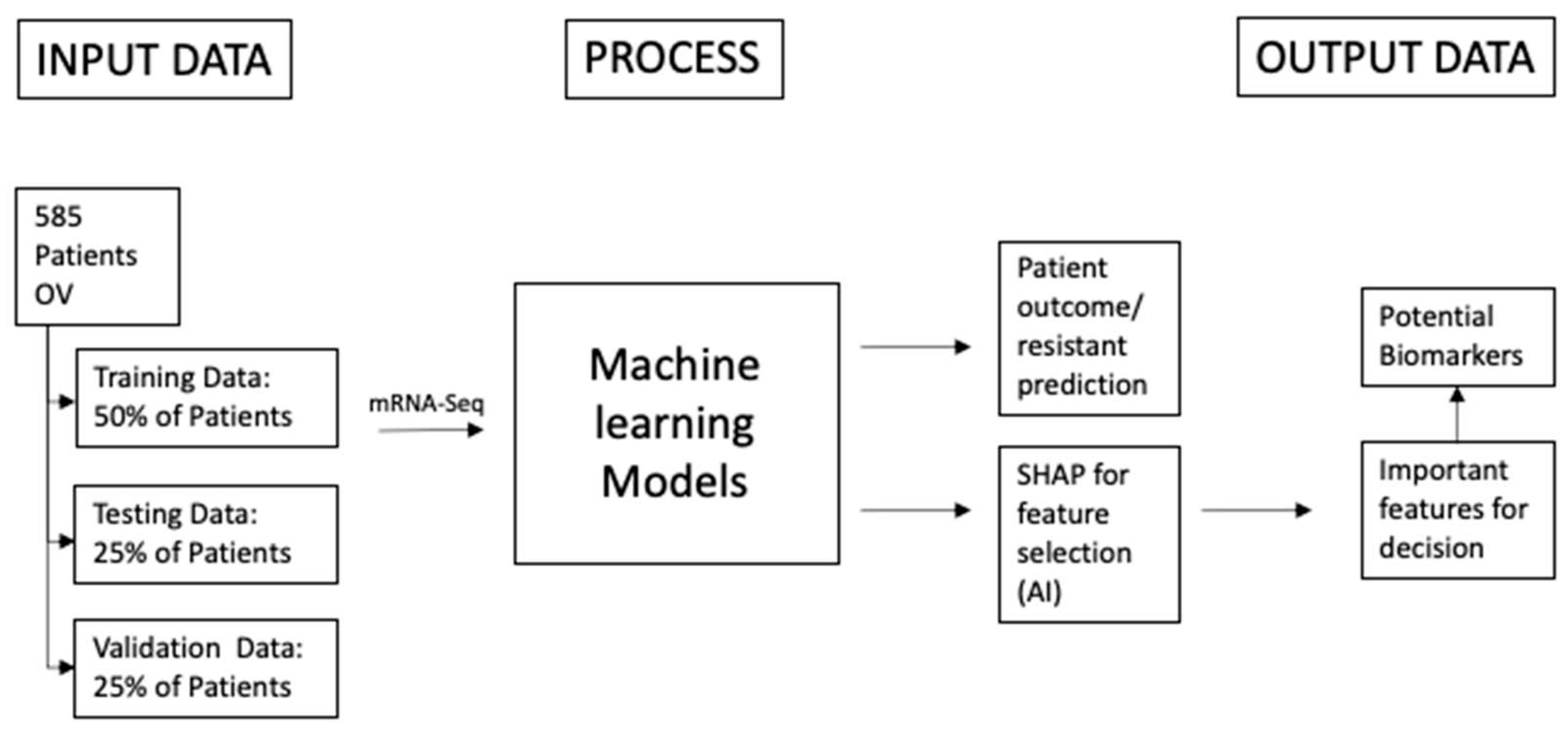
Figure 1. The schematic shows the overall project structure. The study on ovarian cancer consists overall of 585 patients but not for every patient all biological and clinical data is available. The main idea is that the patients will be put into two very distinct categories for example: good outcome, bad outcome or resistant and sensitive. After putting the patients into two classes they will be distributed into three datasets: 50% Training Data, 25% Testing Data and 25% Validation Data. With that method there won't be underlying fitting to the data when the models are getting adjusted and tested. The performance of the models will be determined with a one-time test on the validation data set. The patients and their features are the input for the machine learning models. They should predict the class of the patients. After that when the performance of the models is sufficient algorithms from the field of explainable artificial intelligence will be applied to detect which biological features contribute the most to the decision of the model. Those features will most likely have a biological implication why the patient is having a good or bad outcome.

2. Materials and Methods

2.1. Materials

The data used in the analysis is from the cancer genome atlas (TCGA) [14,15]. It consists of 585 ovarian cancer patients. The unnormalized gene counts for the mRNA sequencing data from GDAC is used for differential gene expression analysis with DESeq2 [16]. Apart from the raw gene counts the clinical data of the patients has been collected to determine whether the patients had a good or bad outcome and if they developed a platinum resistance or were sensitive for it.

Due to limitations in available data, the outcome determination and platinum resistance status were not available for all patients in this study. To address this, two approaches were taken. For the first approach, patients were filtered based on the availability of mRNA sequencing data and their classification as either having a good or bad outcome. In the second approach, patients were required to have both mRNA sequencing data and platinum resistance status available. After filtering, the remaining patient data was randomly divided into training, testing, and independent validation datasets. The training dataset was utilized to train the machine learning models, whereas the testing dataset was used to test the performance of these models in multiple trials. Finally, the validation dataset was employed to evaluate the performance of the models on data that was not previously used for training or testing.

2.1.1. Data on the outcome of the patients:

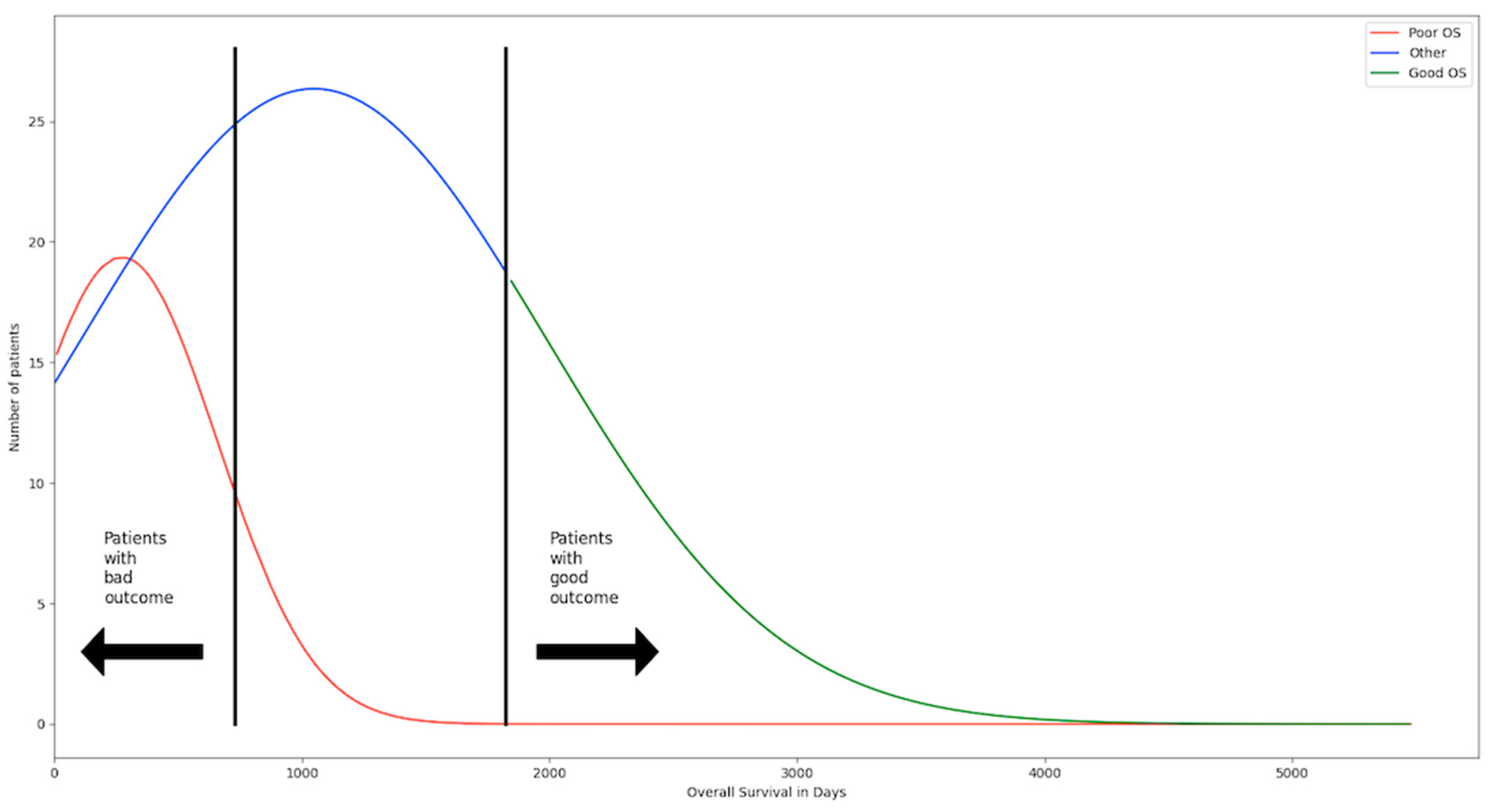
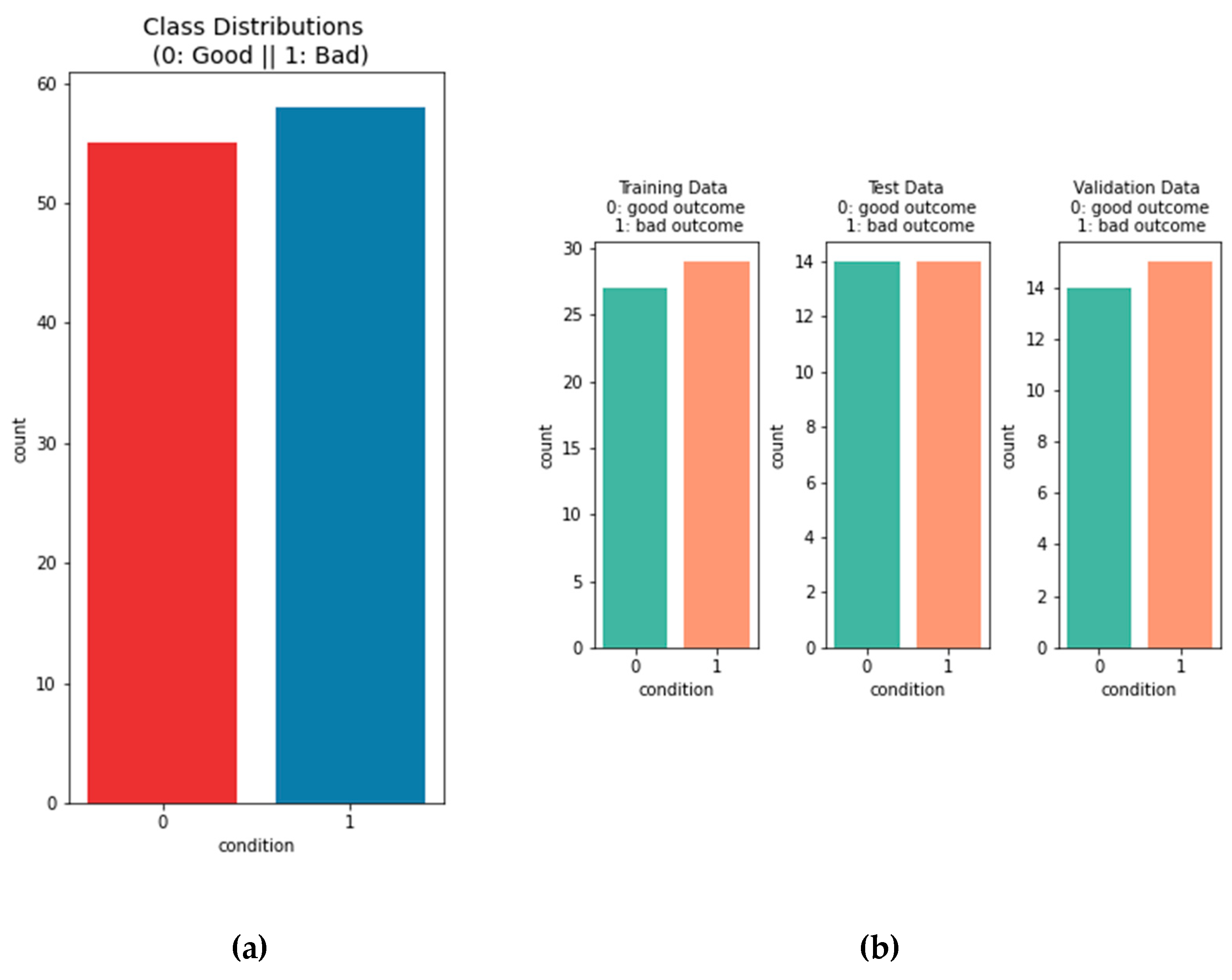
To identify potential biomarkers for ovarian cancer, clear differentiation between patients with good and bad outcome following treatment is essential. As such, patients were classified as having a bad outcome if they had died within two years after treatment, while those who survived for five years or more were classified as having a good outcome. These specific timeframes were selected in order to facilitate clear separation between the patient groups, enabling more distinct differential gene expression analysis. The study cohort included a total of 113 patients, of which 55 were classified as having a good outcome and 58 as having a bad outcome.

Figure 2. The patients have been separated in three groups. The first group are the patients with poor overall survival (OS) and consists of 112 patients. They died within the first two years after treatment and are considered to have a bad outcome. The second group are the patients with positive OS and consists of 119 patients. They have lived five years and longer after treatment and are considered to have a good outcome. The third group are all the patients in between the two groups and make up the biggest portion with 345. Those patients cannot be considered good or bad outcome. The threshold has been selected to have two groups that are very distinct from one another to make changes and differences in their gene expression profile easier to detect.

Figure 2. The patients have been separated in three groups. The first group are the patients with poor overall survival (OS) and consists of 112 patients. They died within the first two years after treatment and are considered to have a bad outcome. The second group are the patients with positive OS and consists of 119 patients. They have lived five years and longer after treatment and are considered to have a good outcome. The third group are all the patients in between the two groups and make up the biggest portion with 345. Those patients cannot be considered good or bad outcome. The threshold has been selected to have two groups that are very distinct from one another to make changes and differences in their gene expression profile easier to detect.

2.1.2. Data on the resistance status of the patients:

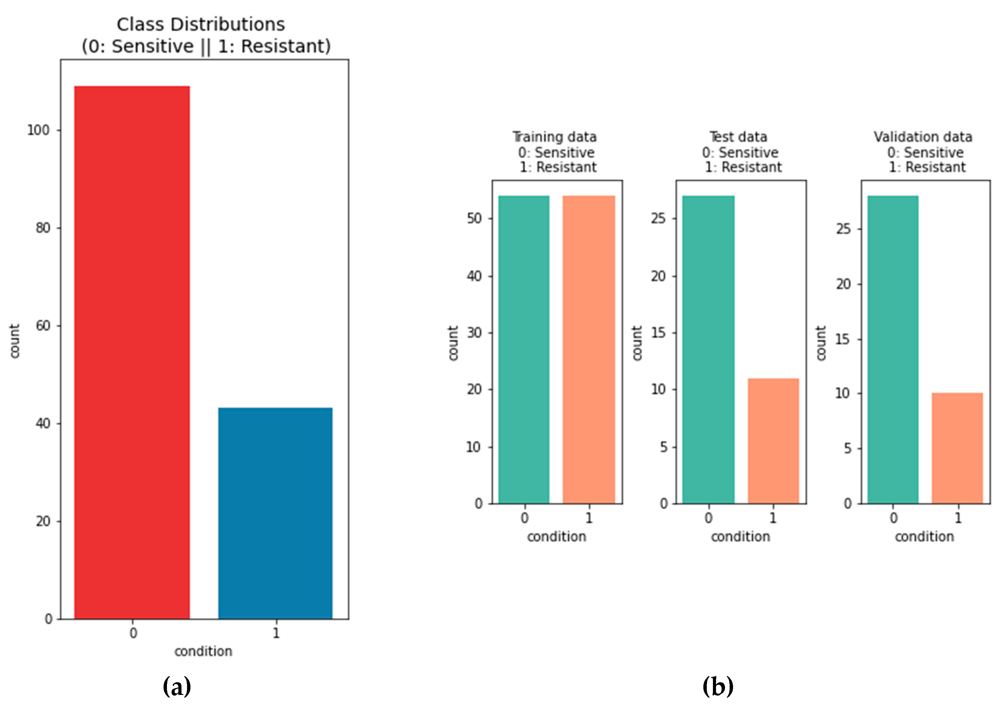
To identify genes that could predict the platinum sensitivity in ovarian cancer the categorization from the TCGA has been used. In total there are 152 patients. 109 of those are sensitive and 43 are resistant.

2.2. Methods

2.2.1. Machine learning methods:

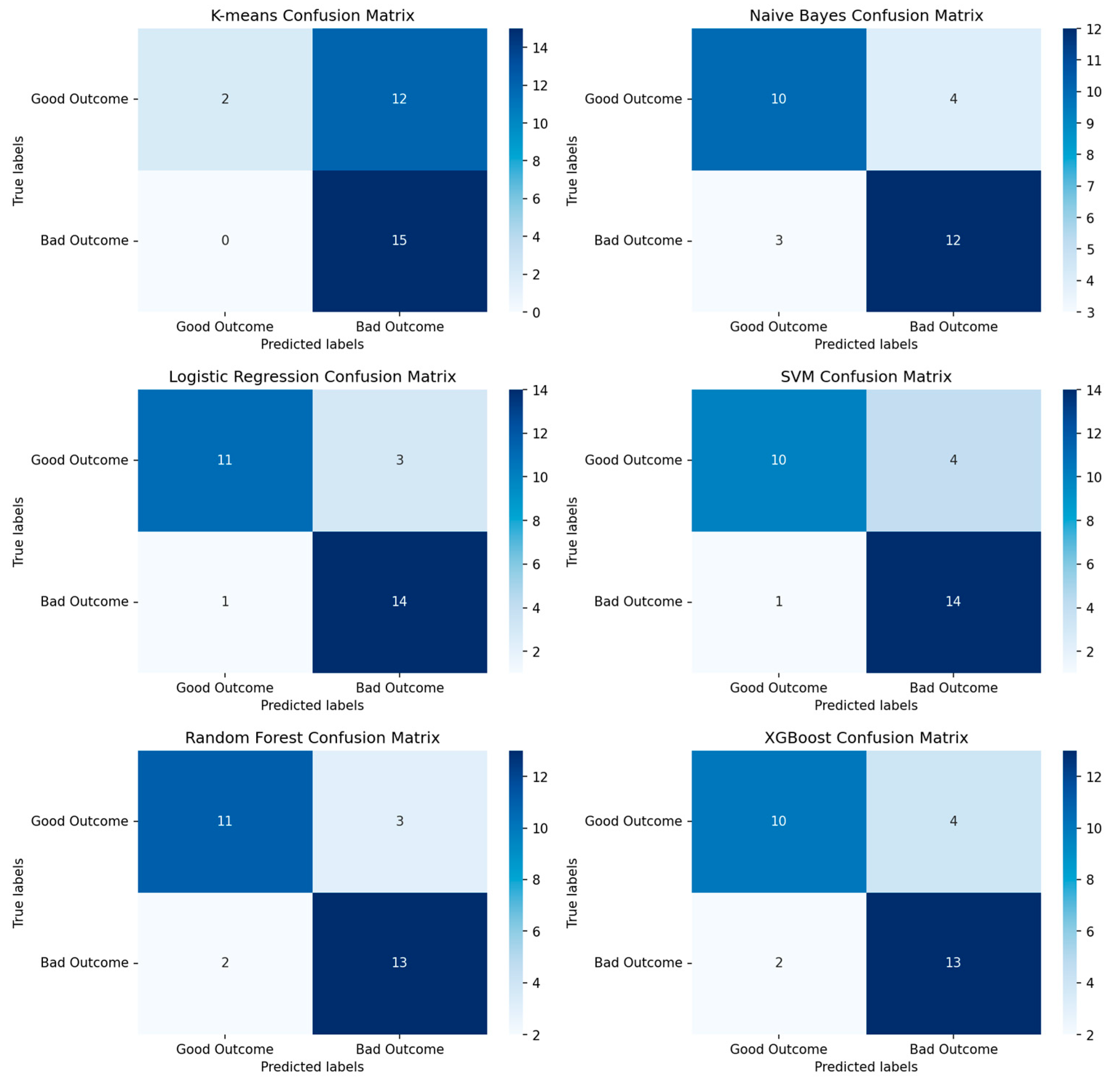
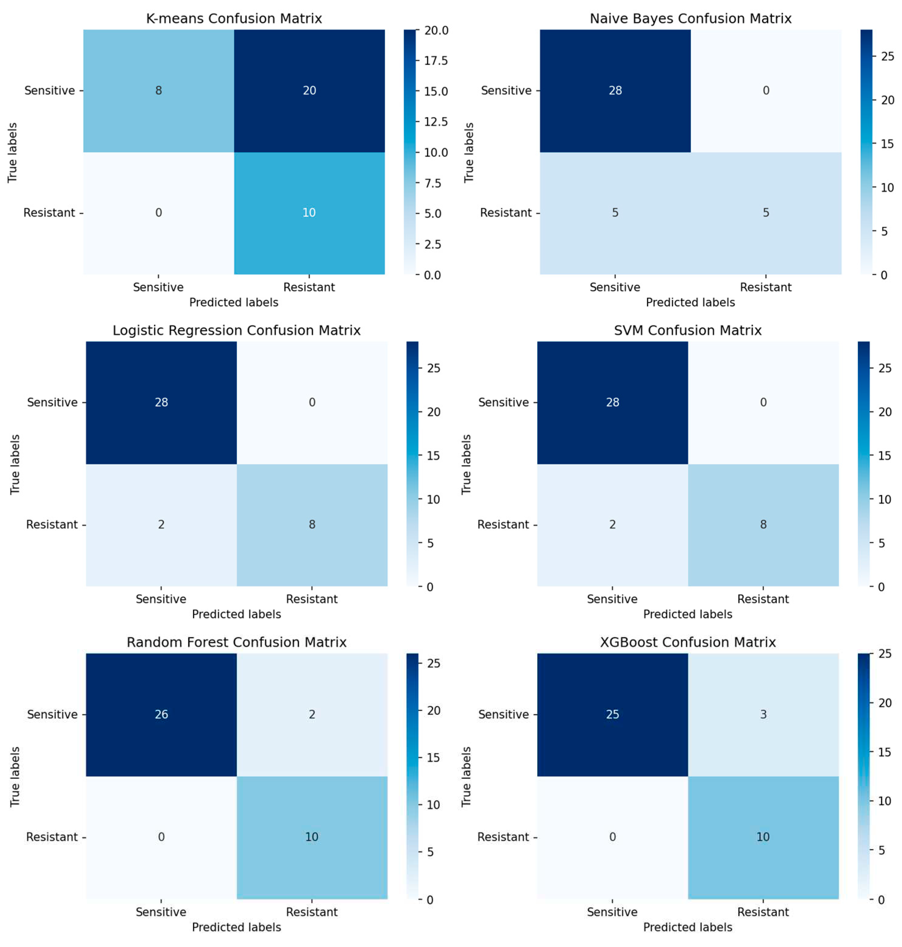
The machine learning methods have been all trained with 50% of the data from each dataset and then frequently tested on 25% of the remaining ones. When the performance reached the desired value it has been tested ones on the remaining 25% to evaluate how well the method performs on unseen data. All of the methods have been trained as binary classifier to identify the correct class by their gene expression profile. The models have been tested with the normalized data and data from the principal component analysis. The training of the models has been done in different Jupyter Notebooks on the “cancer genomics cloud”. For each machine learning model the f1-score has been calculated to determine their predictive performance. In the result part the confusion matrix of the classifiers are depicted to see how their classification performance is distributed via the two classes. The machine learning methods that have been used are: K-means clustering [17,18], Naïve Bayes [19], logistic regression [20,21,22], supported vector machines [23,24], Random Forest [25,26] and XBGoost [27]. All the used methods were integrated via the sklearn library in python. Different hyperparameters have been used to adjust the model to the gene expression data.

2.2.2. SHAP

To determine which genes can be used as biomarkers the XAI method SHAP is used. It utilizes the mathematics from game theory to determine the global significance of the genes for the decision making of the model. After the model has been trained each gene will be given a Shapley value the determines their significance and depending on their overall expression between the two classes it can be assessed if the expression of the gene is correlated to the outcome or platinum resistant status of a patient [28].

2.2.3. Bioinformatics algorithms

The original gene expression data consists of 20429 genes. Most of them are likely not relevant in the search of biomarkers because they will have no biological function associated with the fitness of the cancer. Those genes will not be differentially expressed between the two classes. DESeq2 is a software available in R used to determine differentially expressed genes between two groups. Unnormalized gene counts are used for that purpose. Afterwards the log2fold shrinkage method apeglm is used to determine which genes have significant changes between the two groups [29]. The p-adjusted value is used to select the genes that are significantly expressed between the two groups. A p-adjusted value of 0.01 for the outcome group has been set and 0.05 for the platinum resistant status group. For the outcome group, genes upregulated in patients with a good outcome have a log2foldchange above zero and the ones upregulated in patients with bad outcome have a log2foldchange lower than zero. For the platinum resistant status group, genes upregulated in patients that are platinum sensitive have a log2foldchange above zero and the ones that are upregulated in patients that are platinum resistant have a log2foldchange lower than zero. The selected gene lists will be further analyzed to determine their biological implications in relation to ovarian cancer.

Figure 3. (a) The volcano plot depicted shows the differentially expressed genes between the patients with bad outcome and good outcome. The dots in blue represent genes that have a adjusted p-value of 0.01> and a log2FoldChange between +2 and –2. It means that they are significantly differentially expressed. The red dots represent genes that have a adjusted p-value of 0.01> and a log2FoldChang >2 and –2>. It means that they are highly significantly expressed. The black dots are all genes the have a higher adjusted p-value than 0.1. (b) The volcano plot depicted shows the differentially expressed genes between the patients that are sensitive and resistant. The dots in blue represent genes that have a adjusted p-value of 0.05> and a log2FoldChange between +2 and –2. It means that they are significantly differentially expressed. The red dots represent genes that have a adjusted p-value of 0.05> and a log2FoldChang >2 and –2>. It means that they are highly significantly expressed. The black dots are all genes the have a higher adjusted p-value than 0.1.

Figure 3. (a) The volcano plot depicted shows the differentially expressed genes between the patients with bad outcome and good outcome. The dots in blue represent genes that have a adjusted p-value of 0.01> and a log2FoldChange between +2 and –2. It means that they are significantly differentially expressed. The red dots represent genes that have a adjusted p-value of 0.01> and a log2FoldChang >2 and –2>. It means that they are highly significantly expressed. The black dots are all genes the have a higher adjusted p-value than 0.1. (b) The volcano plot depicted shows the differentially expressed genes between the patients that are sensitive and resistant. The dots in blue represent genes that have a adjusted p-value of 0.05> and a log2FoldChange between +2 and –2. It means that they are significantly differentially expressed. The red dots represent genes that have a adjusted p-value of 0.05> and a log2FoldChang >2 and –2>. It means that they are highly significantly expressed. The black dots are all genes the have a higher adjusted p-value than 0.1.

2.2.4. Statistical methods

After the differential gene expression analysis the gene count data is normalized before it can be used by the machine learning methods. Since the data from the ovarian cancer patients has been collected by multiple hospitals it is need the normalize the sample within the gene and the sample itself. The methods for normalization that can be used is either the commonly used z-normalization or the TMM normalization [30]. Both methods have been used and the performance of the machine learning models was better using the TMM normalization method. Even after normalization there were still outliers so statistical method winsorizing has been applied to the data. So the highest 2.5% of the data is replaced with value right below them. After that SMOTE has been used on the training dataset of the platinum resistance status group [31]. Since the dataset is very imbalanced between the patients that are resistant and the ones that are sensitive the machine learning methods will not be performing well since the prediction will be more based on the class that is more frequent instead of the gene expression values. Therefore SMOTE is used to create fake data points between the original data points. With this approach the machine learning models will be trained with similar data as the original data points and won’t lean to majority class while the integrity of the data stays intact. Afterwards all data points for both groups and datasets will be scaled between zero and one because some methods like SVM will perform better with that scaling. On the resulting datasets a PCA is performed since Random Forest and XGBoost classifiers worked better in the approach than without it. This is essentially just for the assessment of the best performer since it is very difficult to transform the principal components later back to the original features [32,33].

Figure 4. The left bar plot depicts the overall distribution on the data . There are 55 patients that are considered to have good outcome and 57 patients that are considered to have a bad outcome. The distribution between the two classes is very even, so there is no need for over- or under-sampling. In the bar plots on the right the distribution of the classes is shown between the training data, test data and validation data.

Figure 4. The left bar plot depicts the overall distribution on the data . There are 55 patients that are considered to have good outcome and 57 patients that are considered to have a bad outcome. The distribution between the two classes is very even, so there is no need for over- or under-sampling. In the bar plots on the right the distribution of the classes is shown between the training data, test data and validation data.

Figure 5. The left bar plot depicts the overall distribution on the data . There are 109 patients that are considered to be sensitive and 43 patients that are considered to be resistant. The distribution between the two classes is uneven. Oversampling is used to adjust that in the trainings data. In the bar plots on the right the distribution of the classes is shown between the training data, test data and validation data. .

Figure 5. The left bar plot depicts the overall distribution on the data . There are 109 patients that are considered to be sensitive and 43 patients that are considered to be resistant. The distribution between the two classes is uneven. Oversampling is used to adjust that in the trainings data. In the bar plots on the right the distribution of the classes is shown between the training data, test data and validation data. .

3. Results

3.1. Outcome prediction of ovarian cancer patients

3.1.1. Machine learning models performance:

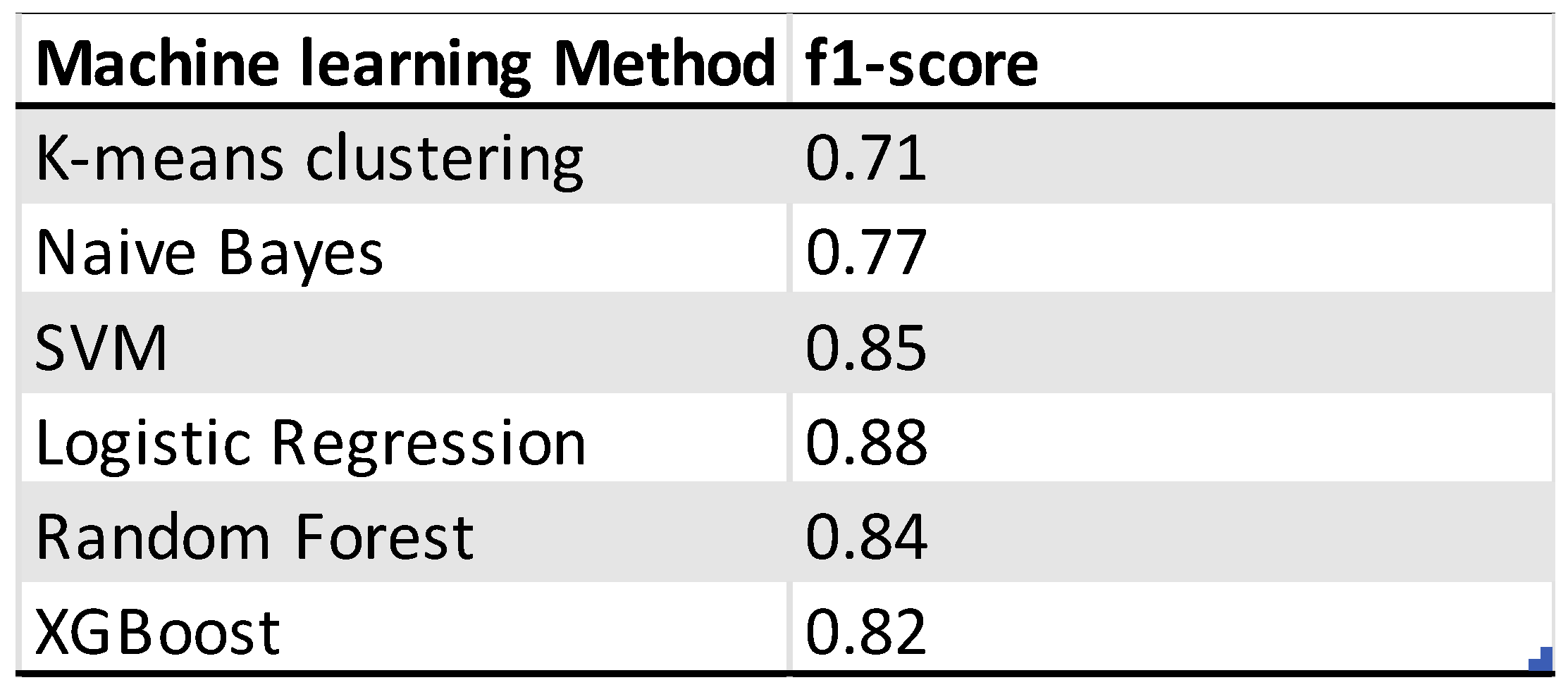
Six different machine learning methods were used to predict the outcome of ovarian cancer patients. The performance is evaluated by the f1-score of the model on the validation dataset. The best performing model is the logistic regression model with 4 misclassifications out of 29 observations. The performance of the other models were slightly lower. The worst performing model is the K-means-clustering model. For the selection of the genes the models have been tested on the differentially expressed genes with a p-adjusted value of 0.1, 0.05 and 0.01. The gene dataset with a cutoff of 0.01 consisting of 149 genes was the best performing one.

Figure 6. Depicted confusion matrixes for the different machine learning methods which have been used. The higher the number for the corresponds between true labels and predicted labels the more accurate and trustworthy the model is. Following are the f1-scores that evaluates the performance of the model: K-means Clustering: 0.71, Naïve Bayes: 0.77, Logistic Regression: 0.88, Supported Vector Machine: 0.85, Random Forest: 0.84, XGBoost: 0.82. The logistic regression model is the model with the highest f1-score and 4 misclassifications from 29 observations.

Figure 6. Depicted confusion matrixes for the different machine learning methods which have been used. The higher the number for the corresponds between true labels and predicted labels the more accurate and trustworthy the model is. Following are the f1-scores that evaluates the performance of the model: K-means Clustering: 0.71, Naïve Bayes: 0.77, Logistic Regression: 0.88, Supported Vector Machine: 0.85, Random Forest: 0.84, XGBoost: 0.82. The logistic regression model is the model with the highest f1-score and 4 misclassifications from 29 observations.

Table 1. Overview of the performance of machine learning models for the outcome prediction of ovarian cancer patients.

Table 1. Overview of the performance of machine learning models for the outcome prediction of ovarian cancer patients.

3.1.2. Identified genes

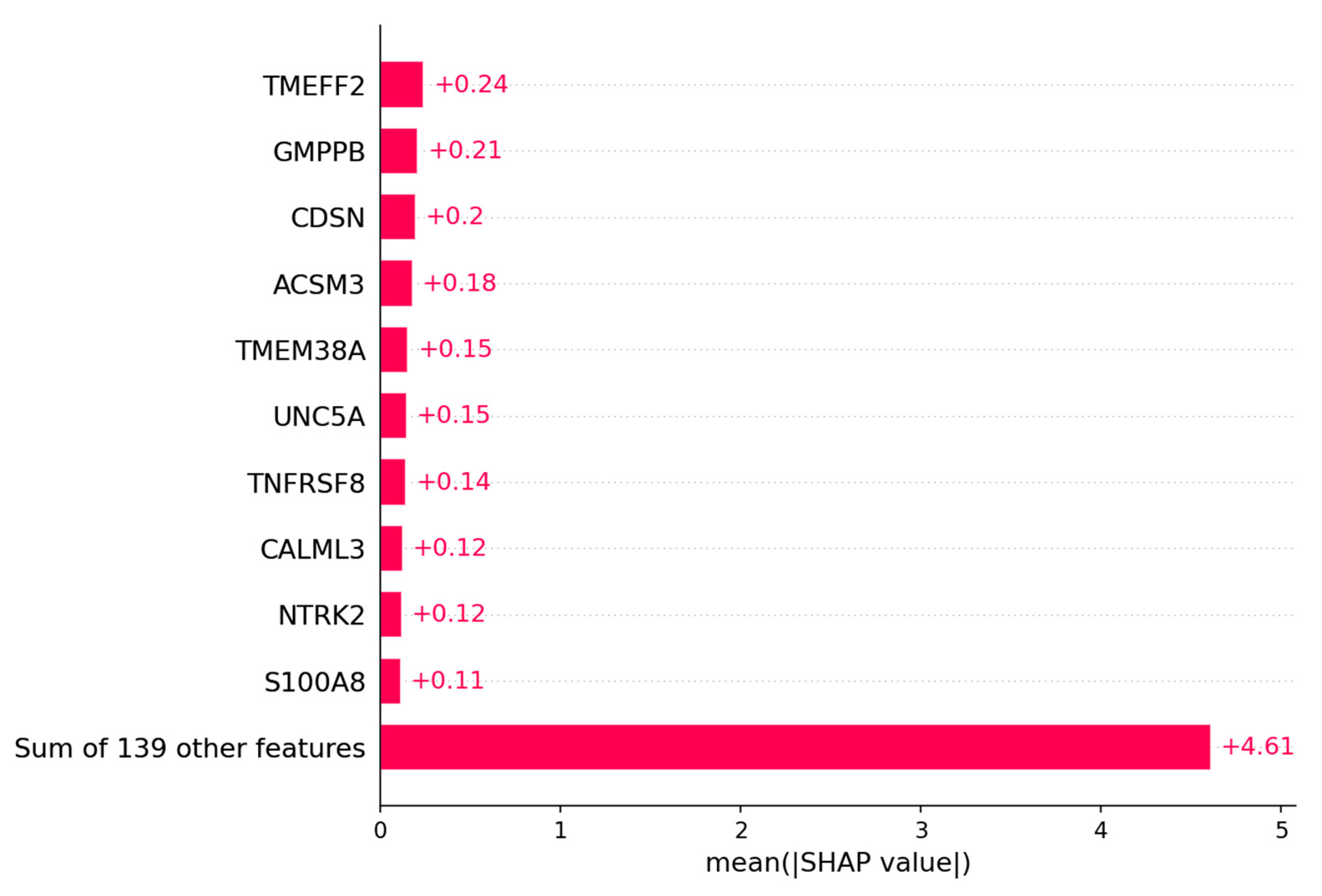
The SHAP Algorithm has been performed on the logistic regression model to evaluate which genes have the highest impact on the outcome of the model. The genes with the highest impact on the model are depicted in Figure 7A. The top 20 genes with the highest Shapley values can be found in Figure A1. Those genes were then separated into the ones that are upregulated in the good outcome group and those that are upregulated in the bad outcome group. Upregulated in this context means the overall expression of that gene is higher in one group of patients than in the other. 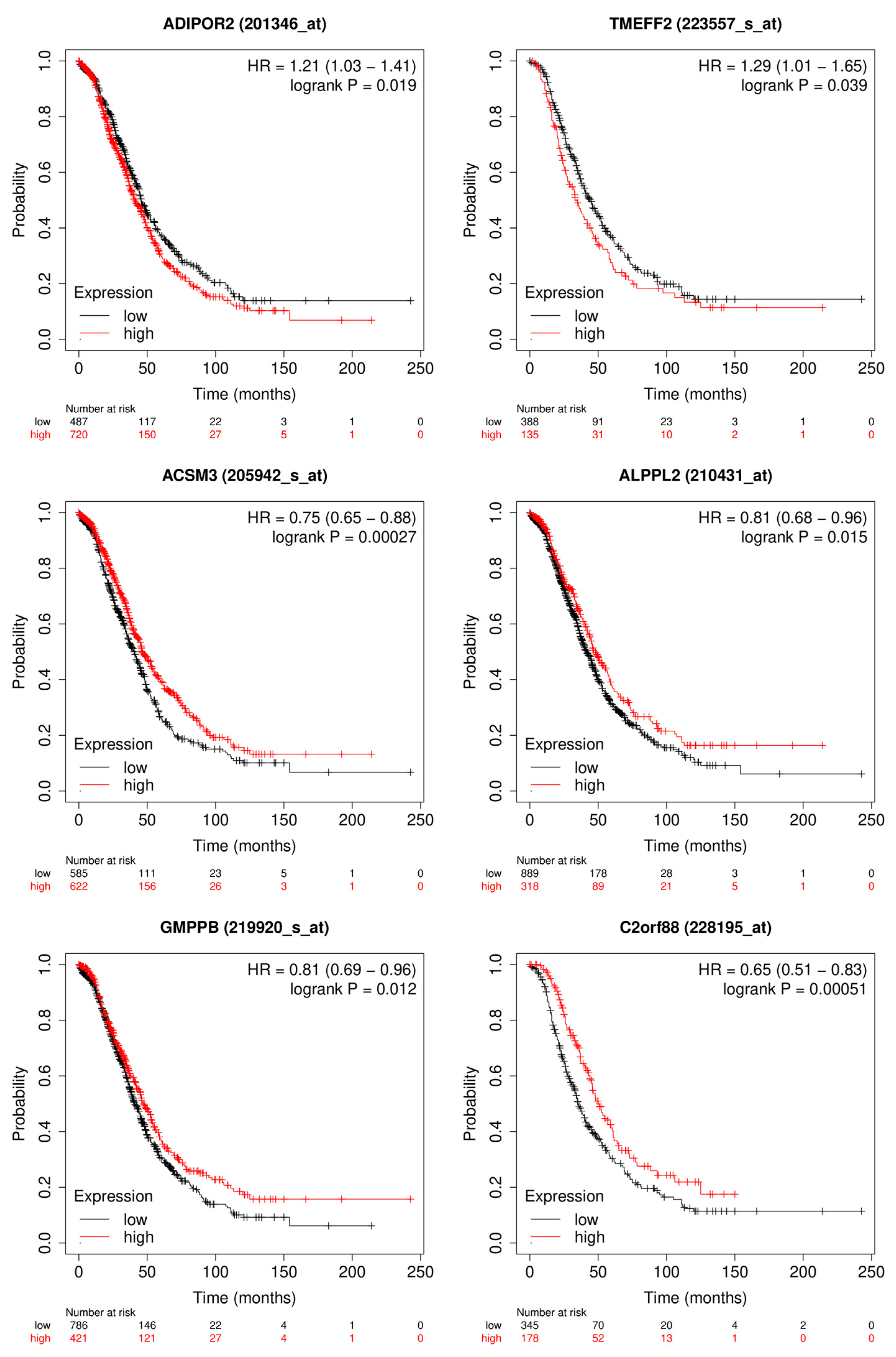In Figure 7B the Kaplan-Meier plots are depicted from six genes with high Shapley values and low adjusted p-values [34]. The first two are upregulated in the group of patients with bad outcome and the other four are upregulated in the group of patients with good outcome.

Figure 7. The bar plot shows the top 10 genes based on the mean SHAP value of the logistic regression model of the ovarian cancer outcome prediction.

Figure 7. The bar plot shows the top 10 genes based on the mean SHAP value of the logistic regression model of the ovarian cancer outcome prediction.

Figure 8. Depicted are the Kaplan-Meier plots for OS of the most relevant genes for the logistic regression model. The genes: ADIPOR2 and TMEFF2 are upregulated in the group of patients with bad outcome. The genes: ACSM3, ALPPL2, GMPPB and C2orf88 are upregulated in the group of patients with good outcome.

Figure 8. Depicted are the Kaplan-Meier plots for OS of the most relevant genes for the logistic regression model. The genes: ADIPOR2 and TMEFF2 are upregulated in the group of patients with bad outcome. The genes: ACSM3, ALPPL2, GMPPB and C2orf88 are upregulated in the group of patients with good outcome.

3.2. Platinum resistance prediction of ovarian cancer patients

3.2.1. Machine Learning Models Performance

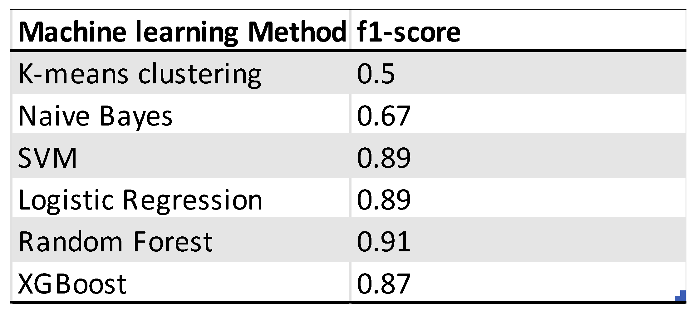
As for the outcome prediction the same six machine learning methods have been used to predict whether a patient is platinum sensitive or resistant. The f1-score is used here as well to assess the performance of the models. The random forest model is the one with the highest f1-score of 0.91 and two misclassifications from 38 observations. The logistic regression model has an f1-score of 0.89 and two misclassifications. The random forest model used the data from the PCA and is therefore more difficult to interpret. For the feature analysis with SHAP the logistic regression model is used instead. The K-means clustering model is here the worst performing model as well. For the selection of the genes the models have been tested on the differentially expressed genes with a p-adjusted value of 0.1 and 0.05. The gene dataset with a cutoff of 0.05 consisting of 172 genes was the best performing one.

Figure 9. Depicted confusion matrixes for the different machine learning methods which have been used. The higher the number for the corresponds between true labels and predicted labels the more accurate and trustworthy the model is. Following are the f1-scores that evaluates the performance of the model: K-means Clustering: 0.5, Naïve Bayes: 0.67, Logistic Regression: 0.89, Supported Vector Machine: 0.89, Random Forest: 0.91, XGBoost: 0.87​. The random forest model is the model with the highest f1-score and two misclassifications from 38 observations.​ For higher interpretability the logistic regression model is used for further analysis.

Figure 9. Depicted confusion matrixes for the different machine learning methods which have been used. The higher the number for the corresponds between true labels and predicted labels the more accurate and trustworthy the model is. Following are the f1-scores that evaluates the performance of the model: K-means Clustering: 0.5, Naïve Bayes: 0.67, Logistic Regression: 0.89, Supported Vector Machine: 0.89, Random Forest: 0.91, XGBoost: 0.87​. The random forest model is the model with the highest f1-score and two misclassifications from 38 observations.​ For higher interpretability the logistic regression model is used for further analysis.

Table 2. Overview of the performance of machine learning models for the platinum resistance status prediction of ovarian cancer patients.

Table 2. Overview of the performance of machine learning models for the platinum resistance status prediction of ovarian cancer patients.

3.2.2. Identified genes

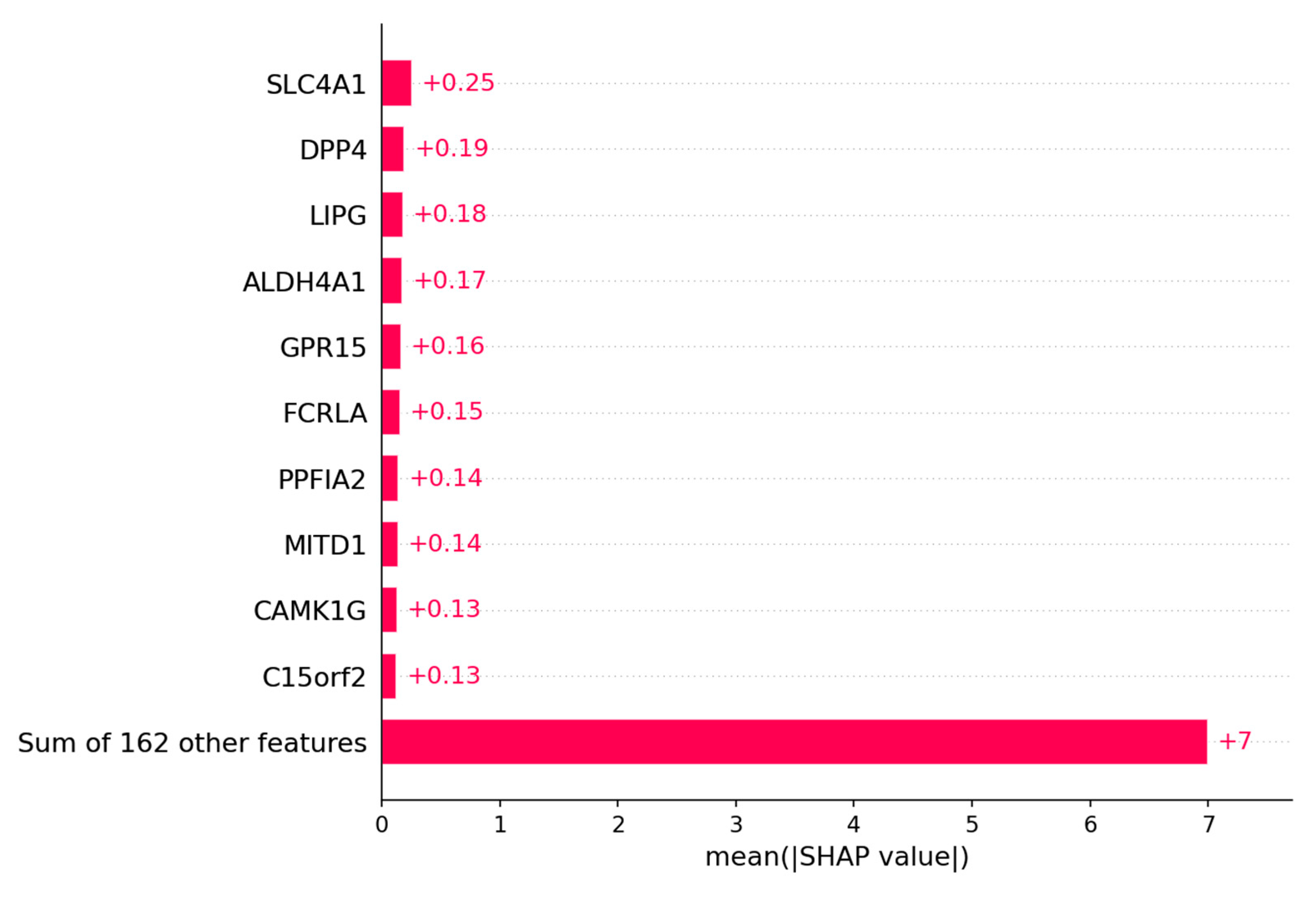
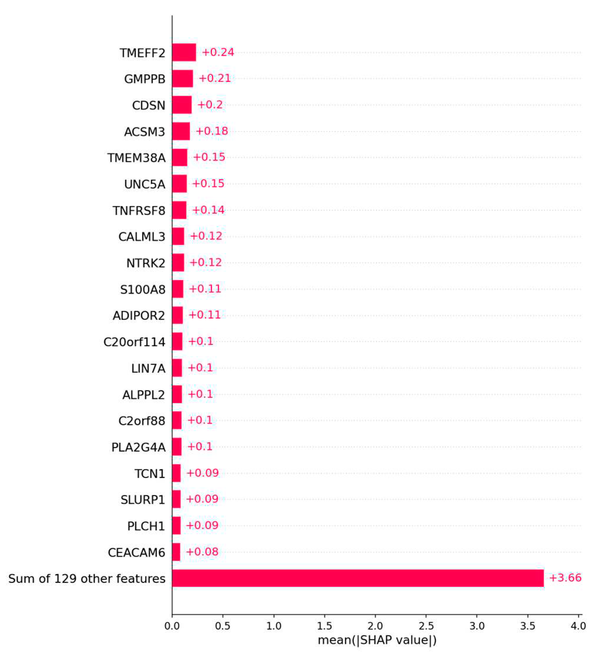
For the selections of genes the SHAP algorithm has been performed on the logistic regression model to evaluate which genes have the highest impact on the prediction whether the patient is platinum sensitive or resistant. The genes with the highest impact on the model are depicted in Figure 9A. The top 20 genes with the highest Shapley values can be found in the Figure 2A. Those genes were then separated into the ones that are upregulated in the patient group that is platinum sensitive and those that are upregulated in the platinum resistant group. In Figure 9B the Kaplan-Meier plots are depicted from six genes with high Shapley values and low adjusted p-values. The first two are upregulated in the group of patients with bad outcome and the other four are upregulated in the group of patients with good outcome.

Figure 10. The bar plot shows the top 10 genes based on the mean SHAP value of the logistic regression model of the platinum resistance prediction.

Figure 10. The bar plot shows the top 10 genes based on the mean SHAP value of the logistic regression model of the platinum resistance prediction.

Figure 11. Depicted are the Kaplan-Meier plots for progression free survival (PFS) of the most relevant genes for the logistic regression model. The genes: ALDH4A1, MITD1 and SLC4A1 (SW) are upregulated in the patients with a platinum resistance. The genes: CAMK1G, GPR15 and PPFIA2 are upregulated in the patients that are platinum sensitive.

Figure 11. Depicted are the Kaplan-Meier plots for progression free survival (PFS) of the most relevant genes for the logistic regression model. The genes: ALDH4A1, MITD1 and SLC4A1 (SW) are upregulated in the patients with a platinum resistance. The genes: CAMK1G, GPR15 and PPFIA2 are upregulated in the patients that are platinum sensitive.

4. Discussion

5. Conclusions

References

1. Ovarian Cancer Survival Rates | Ovarian Cancer Prognosis Available online: https://www.cancer.org/cancer/ovarian-cancer/detection-diagnosis-staging/survival-rates.html (accessed on 26 April 2023).
2. Surgery for Recurrent Ovarian Cancer May Help Selected Patients - NCI Available online: https://www.cancer.gov/news-events/cancer-currents-blog/2022/ovarian-cancer-return-surgery-desktop-iii (accessed on 28 March 2023).
3. Flynn, M.J.; Ledermann, J.A. Ovarian Cancer Recurrence: Is the Definition of Platinum Resistance Modified by PARPi and Other Intervening Treatments? The Evolving Landscape in the Management of Platinum-Resistant Ovarian Cancer. Cancer Drug Resist 2022, 5, 424–435. [CrossRef]
4. Jayson, G.C.; Kohn, E.C.; Kitchener, H.C.; Ledermann, J.A. Ovarian Cancer. The Lancet 2014, 384, 1376–1388. [CrossRef]
5. How to Check for Ovarian Cancer | Ovarian Cancer Screening Available online: https://www.cancer.org/cancer/ovarian-cancer/detection-diagnosis-staging/detection.html (accessed on 28 March 2023).
6. Klein, M.E.; Dabbs, D.J.; Shuai, Y.; Brufsky, A.M.; Jankowitz, R.; Puhalla, S.L.; Bhargava, R. Prediction of the Oncotype DX Recurrence Score: Use of Pathology-Generated Equations Derived by Linear Regression Analysis. Mod Pathol 2013, 26, 658–664. [CrossRef]
7. Kumar, L.; Greiner, R. Gene Expression Based Survival Prediction for Cancer Patients—A Topic Modeling Approach. PLOS ONE 2019, 14, e0224446. [CrossRef]
8. Cardoso, F.; van’t Veer, L.J.; Bogaerts, J.; Slaets, L.; Viale, G.; Delaloge, S.; Pierga, J.-Y.; Brain, E.; Causeret, S.; DeLorenzi, M.; et al. 70-Gene Signature as an Aid to Treatment Decisions in Early-Stage Breast Cancer. New England Journal of Medicine 2016, 375, 717–729. [CrossRef]
9. Tang, Z.; Li, C.; Kang, B.; Gao, G.; Li, C.; Zhang, Z. GEPIA: A Web Server for Cancer and Normal Gene Expression Profiling and Interactive Analyses. Nucleic Acids Res 2017, 45, W98–W102. [CrossRef]
10. Mahood, E.H.; Kruse, L.H.; Moghe, G.D. Machine Learning: A Powerful Tool for Gene Function Prediction in Plants. Appl Plant Sci 2020, 8, e11376. [CrossRef]
11. Johnsen, P.V.; Riemer-Sørensen, S.; DeWan, A.T.; Cahill, M.E.; Langaas, M. A New Method for Exploring Gene–Gene and Gene–Environment Interactions in GWAS with Tree Ensemble Methods and SHAP Values. BMC Bioinformatics 2021, 22, 230. [CrossRef]
12. Divate, M.; Tyagi, A.; Richard, D.J.; Prasad, P.A.; Gowda, H.; Nagaraj, S.H. Deep Learning-Based Pan-Cancer Classification Model Reveals Tissue-of-Origin Specific Gene Expression Signatures. Cancers 2022, 14, 1185. [CrossRef]
13. Bi, Y.; Xiang, D.; Ge, Z.; Li, F.; Jia, C.; Song, J. An Interpretable Prediction Model for Identifying N7-Methylguanosine Sites Based on XGBoost and SHAP. Molecular Therapy - Nucleic Acids 2020, 22, 362–372. [CrossRef]
14. Bell, D.; Berchuck, A.; Birrer, M.; Chien, J.; Cramer, D.W.; Dao, F.; Dhir, R.; DiSaia, P.; Gabra, H.; Glenn, P.; et al. Integrated Genomic Analyses of Ovarian Carcinoma. Nature 2011, 474, 609–615. [CrossRef]
15. Weinstein, J.N.; Collisson, E.A.; Mills, G.B.; Shaw, K.R.M.; Ozenberger, B.A.; Ellrott, K.; Shmulevich, I.; Sander, C.; Stuart, J.M. The Cancer Genome Atlas Pan-Cancer Analysis Project. Nat Genet 2013, 45, 1113–1120. [CrossRef]
16. Love, M.I.; Huber, W.; Anders, S. Moderated Estimation of Fold Change and Dispersion for RNA-Seq Data with DESeq2. Genome Biology 2014, 15, 550. [CrossRef]
17. Steinhaus, H. Bulletin de l’acade ́mie polonaise des sciences. October 19 1956, pp. 801–804.
18. Lloyd, S. Least Squares Quantization in PCM. IEEE Trans. Inform. Theory 1982, 28, 129–137. [CrossRef]
19. Bayes, T.; Price, null LII. An Essay towards Solving a Problem in the Doctrine of Chances. By the Late Rev. Mr. Bayes, F. R. S. Communicated by Mr. Price, in a Letter to John Canton, A. M. F. R. S. Philosophical Transactions of the Royal Society of London 1763, 53, 370–418. [CrossRef]
20. Garnier, J.-G.; Quetelet, A. Correspondance mathématique et physique; M.Hayez, imprimeur, 1838;
21. Verhulst, P.-F. NOUVEAUX MÉMOIRES DE L’ACADÉMIE ROYALE DES SCIENCES ET BELLES-LETTRES DE BRUXELLES; L’Académie Royale de Bruxelles et de l’Université Louvain, 1845;
22. Verhulst, P.-F. MÉMOIRES DE L’ACADÉMIE IMPÉRIALE ET ROYALE DES SCIENCES ET BELLES-LETTRES DE BRUXELLES; A. BRUXELLES; DE L’IMPRIMERIE ACADÉMIQUE, 1847;
23. Vapnik, V.N.; Lerner, A.Ya. Recognition of Patterns with help of Generalized Portraits. Recognition of Patterns with help of Generalized Portraits 1963, 24, 774–780.
24. Cortes, C.; Vapnik, V. Support-Vector Networks. Mach Learn 1995, 20, 273–297. [CrossRef]
25. Ho, T.K. Random Decision Forests. In Proceedings of the Proceedings of 3rd International Conference on Document Analysis and Recognition; August 1995; Vol. 1, pp. 278–282 vol.1.
26. Breiman, L. Random Forests. Machine Learning 2001, 45, 5–32. [CrossRef]
27. Chen, T.; Guestrin, C. XGBoost: A Scalable Tree Boosting System. In Proceedings of the Proceedings of the 22nd ACM SIGKDD International Conference on Knowledge Discovery and Data Mining; August 13 2016; pp. 785–794.
28. Lundberg, S.; Lee, S.-I. A Unified Approach to Interpreting Model Predictions 2017.
29. Zhu, A.; Ibrahim, J.G.; Love, M.I. Heavy-Tailed Prior Distributions for Sequence Count Data: Removing the Noise and Preserving Large Differences. Bioinformatics 2019, 35, 2084–2092. [CrossRef]
30. Robinson, M.D.; Oshlack, A. A Scaling Normalization Method for Differential Expression Analysis of RNA-Seq Data. Genome Biology 2010, 11, R25. [CrossRef]
31. Chawla, N.V.; Bowyer, K.W.; Hall, L.O.; Kegelmeyer, W.P. SMOTE: Synthetic Minority over-Sampling Technique. J. Artif. Int. Res. 2002, 16, 321–357.
32. Pearson, K. LIII. On Lines and Planes of Closest Fit to Systems of Points in Space. The London, Edinburgh, and Dublin Philosophical Magazine and Journal of Science 1901, 2, 559–572. [CrossRef]
33. Hotelling, H. Analysis of a Complex of Statistical Variables into Principal Components. Journal of Educational Psychology 1933, 24, 417–441. [CrossRef]
34. Kaplan, E.L.; Meier, P. Nonparametric Estimation from Incomplete Observations. Journal of the American Statistical Association 1958, 53, 457–481. [CrossRef]
35. Gao, L.; Nie, X.; Zheng, M.; Li, X.; Guo, Q.; Liu, J.; Liu, Q.; Hao, Y.; Lin, B. TMEFF2 Is a Novel Prognosis Signature and Target for Endometrial Carcinoma. Life Sciences 2020, 243, 116910. [CrossRef]
36. Alabiad, M.A.; Harb, O.A.; Hefzi, N.; Ahmed, R.Z.; Osman, G.; Shalaby, A.M.; Alnemr, A.A.-A.; Saraya, Y.S. Prognostic and Clinicopathological Significance of TMEFF2, SMOC-2, and SOX17 Expression in Endometrial Carcinoma. Experimental and Molecular Pathology 2021, 122, 104670. [CrossRef]
37. Tiwari, A.; Ocon-Grove, O.M.; Hadley, J.A.; Giles, J.R.; Johnson, P.A.; Ramachandran, R. Expression of Adiponectin and Its Receptors Is Altered in Epithelial Ovarian Tumors and Ascites-Derived Ovarian Cancer Cell Lines. International Journal of Gynecologic Cancer 2015, 25. [CrossRef]
38. Yan, L.; He, Z.; Li, W.; Liu, N.; Gao, S. The Overexpression of Acyl-CoA Medium-Chain Synthetase-3 (ACSM3) Suppresses the Ovarian Cancer Progression via the Inhibition of Integrin Β1/AKT Signaling Pathway. Front Oncol 2021, 11, 644840. [CrossRef]
39. Yang, X.; Wu, G.; Zhang, Q.; Chen, X.; Li, J.; Han, Q.; Yang, L.; Wang, C.; Huang, M.; Li, Y.; et al. ACSM3 Suppresses the Pathogenesis of High-Grade Serous Ovarian Carcinoma via Promoting AMPK Activity. Cell Oncol. 2022, 45, 151–161. [CrossRef]
40. Su, Y.; Zhang, X.; Bidlingmaier, S.; Behrens, C.R.; Lee, N.-K.; Liu, B. ALPPL2 Is a Highly Specific and Targetable Tumor Cell Surface Antigen. Cancer Res 2020, 80, 4552–4564. [CrossRef]
41. Liu, J.; Li, S.; Feng, G.; Meng, H.; Nie, S.; Sun, R.; Yang, J.; Cheng, W. Nine Glycolysis-Related Gene Signature Predicting the Survival of Patients with Endometrial Adenocarcinoma. Cancer Cell International 2020, 20, 183. [CrossRef]
42. Bi, J.; Bi, F.; Pan, X.; Yang, Q. Establishment of a Novel Glycolysis-Related Prognostic Gene Signature for Ovarian Cancer and Its Relationships with Immune Infiltration of the Tumor Microenvironment. Journal of Translational Medicine 2021, 19, 382. [CrossRef]
43. C2orf88 Chromosome 2 Open Reading Frame 88 [Homo Sapiens (Human)] - Gene - NCBI Available online: https://www.ncbi.nlm.nih.gov/gene/84281#summary (accessed on 26 April 2023).
44. Nasimian, A.; Ahmed, M.; Hedenfalk, I.; Kazi, J.U. A Deep Tabular Data Learning Model Predicting Cisplatin Sensitivity Identifies BCL2L1 Dependency in Cancer. Computational and Structural Biotechnology Journal 2023, 21, 956–964. [CrossRef]
45. Qin, L.; Li, T.; Liu, Y. High SLC4A11 Expression Is an Independent Predictor for Poor Overall Survival in Grade 3/4 Serous Ovarian Cancer. PLoS One 2017, 12, e0187385. [CrossRef]
46. Zhang, L.-J.; Lu, R.; Song, Y.-N.; Zhu, J.-Y.; Xia, W.; Zhang, M.; Shao, Z.-Y.; Huang, Y.; Zhou, Y.; Zhang, H.; et al. Knockdown of Anion Exchanger 2 Suppressed the Growth of Ovarian Cancer Cells via MTOR/P70S6K1 Signaling. Sci Rep 2017, 7, 6362. [CrossRef]
47. Parks, S.K.; Chiche, J.; Pouysségur, J. Disrupting Proton Dynamics and Energy Metabolism for Cancer Therapy. Nat Rev Cancer 2013, 13, 611–623. [CrossRef]
48. Damaghi, M.; Wojtkowiak, J.; Gillies, R. PH Sensing and Regulation in Cancer. Frontiers in Physiology 2013, 4.
49. Tomita, H.; Tanaka, K.; Tanaka, T.; Hara, A. Aldehyde Dehydrogenase 1A1 in Stem Cells and Cancer. Oncotarget 2016, 7, 11018. [CrossRef]
50. Ginestier, C.; Korkaya, H.; Dontu, G.; Birnbaum, D.; Wicha, M.S.; Charafe-Jauffret, E. [The cancer stem cell: the breast cancer driver]. Med Sci (Paris) 2007, 23, 1133–1139. [CrossRef]
51. Dong, S.; Hou, D.; Peng, Y.; Chen, X.; Li, H.; Wang, H. Pan-Cancer Analysis of the Prognostic and Immunotherapeutic Value of MITD1. Cells 2022, 11, 3308. [CrossRef]
52. Lee, S.; Chang, J.; Renvoisé, B.; Tipirneni, A.; Yang, S.; Blackstone, C. MITD1 Is Recruited to Midbodies by ESCRT-III and Participates in Cytokinesis. Mol Biol Cell 2012, 23, 4347–4361. [CrossRef]
53. Nikolova, D.N.; Doganov, N.; Dimitrov, R.; Angelov, K.; Low, S.-K.; Dimova, I.; Toncheva, D.; Nakamura, Y.; Zembutsu, H. Genome-Wide Gene Expression Profiles of Ovarian Carcinoma: Identification of Molecular Targets for the Treatment of Ovarian Carcinoma. Mol Med Rep 2009, 2, 365–384. [CrossRef]
54. Brzozowski, J.S.; Skelding, K.A. The Multi-Functional Calcium/Calmodulin Stimulated Protein Kinase (CaMK) Family: Emerging Targets for Anti-Cancer Therapeutic Intervention. Pharmaceuticals (Basel) 2019, 12, 8. [CrossRef]
55. Wang, Y.; Wang, X.; Xiong, Y.; Li, C.-D.; Xu, Q.; Shen, L.; Chandra Kaushik, A.; Wei, D.-Q. An Integrated Pan-Cancer Analysis and Structure-Based Virtual Screening of GPR15. Int J Mol Sci 2019, 20, 6226. [CrossRef]
56. PPFIA2 PTPRF Interacting Protein Alpha 2 [Homo Sapiens (Human)] - Gene - NCBI Available online: https://www.ncbi.nlm.nih.gov/gene/8499#summary (accessed on 27 April 2023).