GPR Target Recognition Based on Improved YOLOv3-SPP

Preprint

Article

GPR Target Recognition Based on Improved YOLOv3-SPP

Altmetrics

Downloads

117

Views

Comments

This version is not peer-reviewed

Submitted:

18 May 2023

Posted:

19 May 2023

You are already at the latest version

Alerts

Abstract

When ground-penetrating radar is used to detect targets within concrete, the location of the targets, the identification of different shapes, properties and less obvious echoes all greatly increase the interpretation time of the staff and can easily cause misjudgment of the echo images. In this paper, the ground-penetrating radar echo images (B-scan) after processing are mean filtered to eliminate the direct waves that interfere greatly with the echoes. The RFB-s structure is added to the YOLOv3-SPP network structure, while the Anchor value is optimized and the EIOU loss function is introduced. For four types of data with different shapes and properties at random target locations, three models, YOLOv3, YOLOv3-SPP and the improved YOLOv3-SPP, are used for classification and identification, and the proposed algorithm models are comprehensively evaluated using model evaluation metrics. The experimental results show that the algorithm models proposed in this paper have good recognition effect in ground-penetrating radar echo image target detection.

Keywords:

Subject: Computer Science and Mathematics - Artificial Intelligence and Machine Learning

1. Introduction

Ground-penetrating radar (GPR) is a non-destructive testing method which uses the transmission characteristics of electromagnetic waves to detect underground structures and materials. The technique uses a pair of antennas, one for transmitting electromagnetic waves, and the other for receiving echo signals. When the electromagnetic wave passes through the underground dielectric layer with different attributes, part of the energy will be reflected back. The echo is detected by the receiving antenna, and the characteristics of the echo signal are calculated and analyzed. The image carrying the characteristics of the underground structure can be generated. At present, this method is widely used in road disease detection, underground pipelines, tunnel cavity detection, and many others [1,2,3].

Underground target detection is one of the typical cases in the application of ground-penetrating radar, which can effectively detect voids and steel bars in underground structures [4,5]. However, at present, this technology is not mature enough. Most previous studies have focused on delay estimation and horizon identification [6,7]. Because of the large amount of data generated by GPR, it is necessary to interpret and analyze the data manually, which usually takes a considerable amount of time and energy. In addition, the results of the analysis will also depend on the individual professional level of the staff.

At present, the research in the field of machine learning is developing rapidly, and the target detection algorithm based on the neural network YOLO series [8,9,10] has become a research hotspot in the field of computer vision, such as using a deep learning network to detect surface defects [11], remote sensing images, and traffic signs recognition [12,13], etc., which is showing fast and accurate advantages. Drawing lessons from the idea of feature pyramid FPNs [14] (feature pyramid networks), YOLOv3 uses Darknet-53 as the backbone to output three feature maps of different sizes to detect targets of different sizes, but with the continuous sampling and fusion operations in the network, there may be repeated feature information in different levels of feature maps, which may cause the model to pay too much attention to some specific features and ignore other important features, thus affecting the performance of the model. YOLOv3-SPP encompasses the addition of a spatial pyramid pooling (SPP, [15]) module on the basis of YOLOv3, which replaces the pooling operation of the last layer of Darknet-53, strengthens the ability of extracting global and local features, and has a better effect on small targets and targets with a large aspect ratio. It is the best algorithm model in the YOLOv3 series as it demonstrates a comprehensive performance.

Because the echo image features of bottom detection radar are not obvious, there are many noises and various waveforms. In order to improve the recognition accuracy of the algorithm, this paper uses the YOLOv3-SPP network as the model and makes a series of improvements, such as using the re-clustering algorithm to optimize the corresponding Anchorage value, making the addition of the RFB-s module [16] to fuse image features of different scales, and introducing the EIoU loss function [17] to improve the original loss function. This paper aims to discover the optimal target recognition algorithm in order to improve the accuracy of underground target detection using bottom detection radar.

2. Introduction and Preprocessing of Dataset

2.1 Brief Introduction of Ground-Penetrating Radar

GPR is a technology that uses electromagnetic waves to detect underground objects; it is widely used in exploration, military, geological, environmental monitoring, and other fields. Based on the mechanism that different dielectric interfaces produce different electromagnetic wave reflection signals, the technology uses the transmitting antenna (Tx) to emit electromagnetic waves and the receiving antenna (Rx) to receive the echo signals. Through the analysis and processing of the echo signals, the relevant information of underground objects is obtained. The data produced by one scan of ground-penetrating radar is called A-scan data. By scanning the target area and concatenating the A-scan data, the B-scan data are converted into two-dimensional images, that is, B-scan echo images, which can reflect the depth and shape of underground targets.

2.2 Experimental Real Data

The real data of GPR echo images used in this study derive from the data of road underground targets on the Internet. According to the engineering experience of road disease detection, road underground targets mainly include all kinds of pipelines and crack diseases [18]. Therefore, the real echo images can be divided into three categories: pipeline, disease, and no target, which are 856, 654, and 490 image data, respectively. Three types of images are shown in Figure 1.

Most of the cross sections of all kinds of pipeline targets are circular and usually show a hyperbolic shape in GPR images, as shown in Figure 1A. Diseases include local material voids and looseness between the structural layers, most of which are irregular in shape, which is usually shown as an isolated line in GPR images, with hyperbolic features at the bottom and both ends, as shown in Figure 1b. When there is no target underground, the GPR image contains only the background of direct waves and reflected waves generated by layered underground structures, as shown in Figure 1c.

2.3 GPRMAX Simulation Data

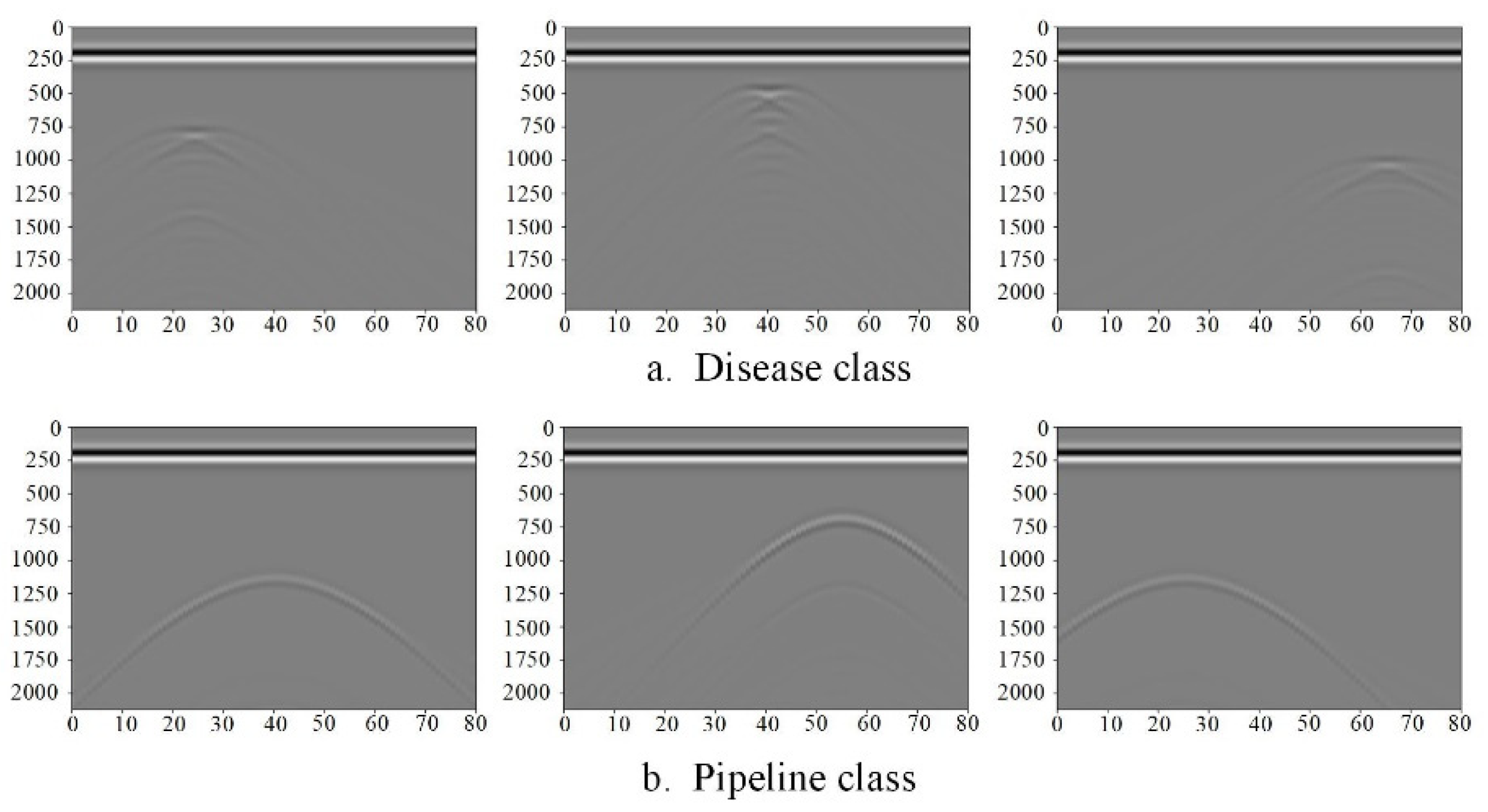
Due to the lack of public image data related to GPR at present, and in order to further explore the difference between real data and theoretical data, this paper first uses GPRMAX to generate corresponding simulation data images to further increase the number of datasets. In this paper, the simulation model is set as pipeline (iron, PVC) and disease (air). The shape of the pipeline target is set to a circle, the radius is 10cm, and the shape of the disease target is set to a rectangle with a small width, and the length and width is 10cm × 2cm to simulate strip disease. As shown in Figure 2, all the target positions are randomly generated; that is, the characteristic positions of all kinds of images are randomly generated in order to enhance the generalization ability of the model. The Abscissa in the figure represents the number of steps of GPR antenna movement, each step is 0.02m, and the ordinate represents the GPR designated time window; that is, the time period from the emission of an electromagnetic wave to its acceptance, in units, is 10e-12s.

Due to the characteristics of GPR, there will be direct waves in the echo data. The characteristics of direct waves are as follows: (1) they are generated at the initial stage of electromagnetic wave transmission, which is earlier than the target echo; (2) the amplitude is much larger than the target echo, so that the target echo is seriously disturbed and even completely covered in the image; and (3) the waveform is relatively stable, and the amplitude and shape are basically unchanged in the B-scan diagram. Direct wave is an interference signal with prominent features which affects the effect of target detection and needs to be filtered. In this paper, the mean filtering method is used to remove the direct wave. Suppose that the B-scan image consists of N A-scan echo data with M sampling points; that is, the B-scan image is an M × N matrix, and the formula is as follows:

{d^{'}}_{i} (j) = d_{i} (j) - \frac{1}{N} \sum_{k = 1}^{N} d_{i} (k), i = 1, ..., M, j = 1, ..., N

(1)

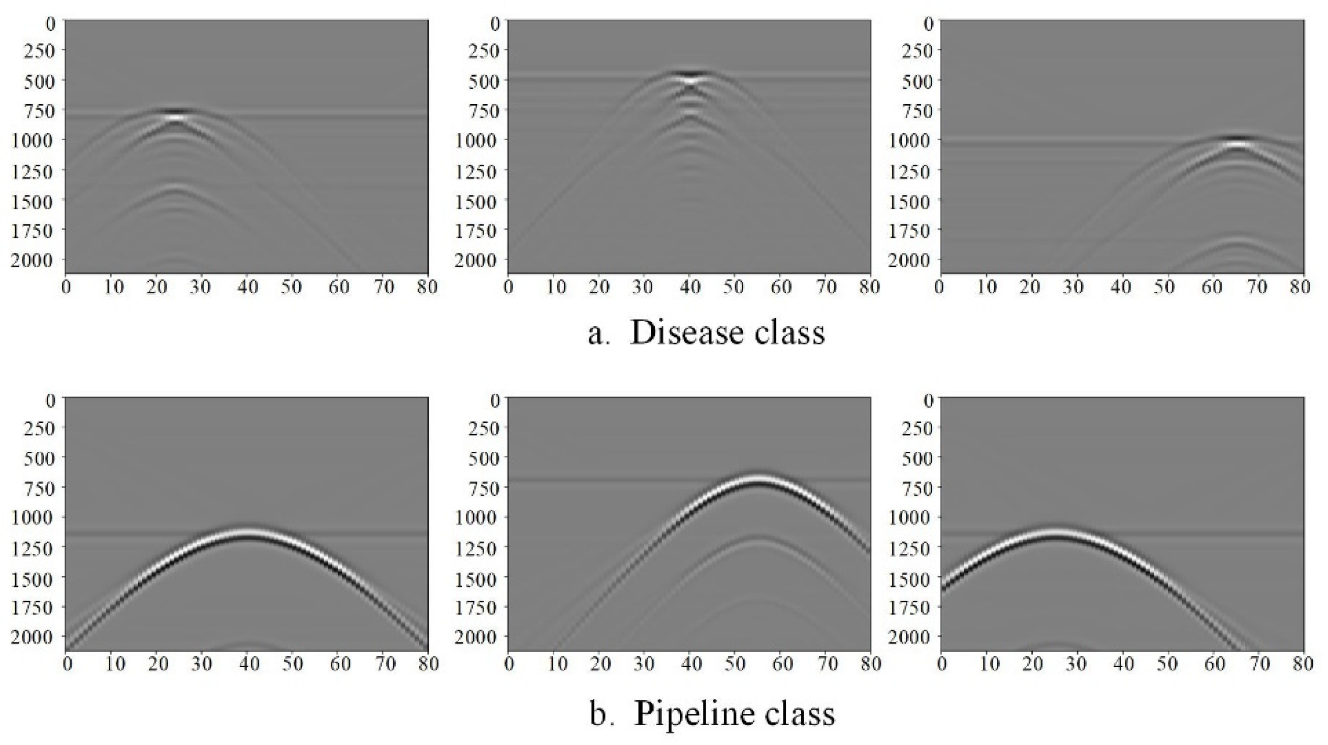
In the formula, di (j) is the j th echo data before processing, and di' (j) is the j echo data after processing. Figure 3 shows the effect of GPR removing direct waves. After removing direct waves, the echo signal is not affected and enhanced, and the characteristics are more obvious, which will make the detection results more accurate.

In this paper, each category of data, according to its different location, generates 1000 B-scan images, showing different morphological characteristics according to the difference in the peak radians, as shown in Figure 3. The main difference between the echo characteristics of diseases and pipelines is that the echo of the pipeline is a smooth hyperbola, while the top of the arc of the disease is a line, and there is a hyperbola at the bottom and both ends of the line. In brief, the echo characteristics of the GPRMAX simulation image data are consistent with the real GPR image data, which shows that the discrimination criterion of the target echo characteristics in a real road underground structure is reliable.

3. Introduction and Improvement of YOLOv3-SPP Algorithm

3.1 YOLOv3-SPP

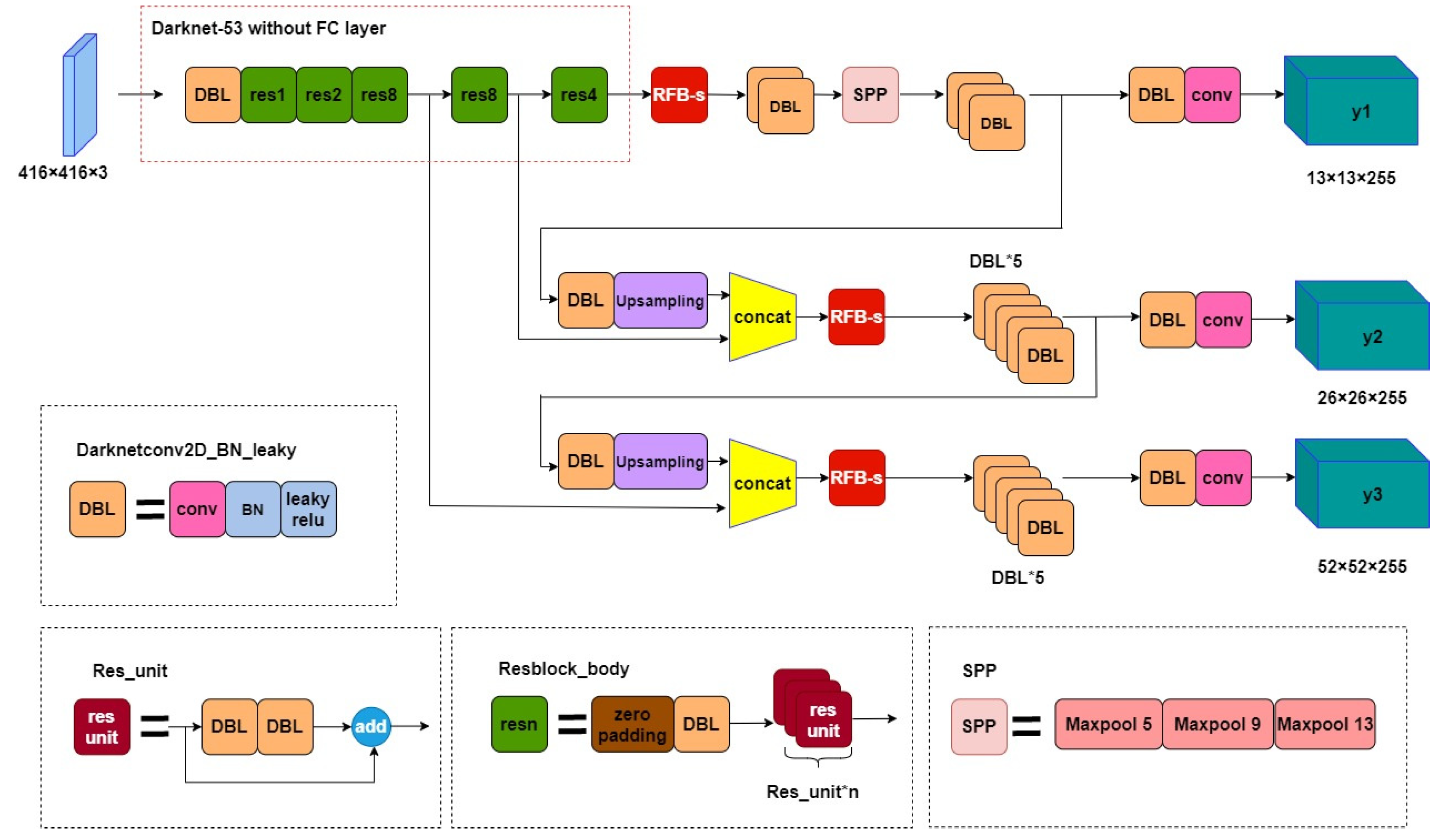
From YOLOv2 to YOLOv3, the original darknet-19 network structure is changed to the Darknet-53 network structure, and the target detection problem is transformed into a regression problem, replacing the original softmax. As the backbone of the whole network structure, Darknet-53 controls the output size by increasing the step size of the convolution kernel. YOLOv3 outputs three feature images of different sizes, draws lessons from the idea of FPN, and adopts the method of up-sampling and feature fusion to enhance the feature mining ability of the model. YOLOv3-SPP disassembles and inserts the SPP module at the DBL where the first prediction feature map passes, draws lessons from the idea of a spatial pyramid, uses multiple parallel branches to learn features of different scales, and realizes the fusion of global features and local features.

The formula of the YOLOv3 loss function is:

L o s s = l_{b o x} + l_{o b j} + l_{c l s}

(2)

In Formula (2),

l_{b o x}

is the predicted position loss, and the specific expression is:

l_{b o x} = λ_{c o r d} \sum_{i = 1}^{S^{2}} \sum_{j = 1}^{B} I_{i, j}^{o b j} (2 - w_{i} \times h_{i}) \times \cdot \cdot \cdot \times [{(x_{i} - {\overset{⌢}{x}}_{i})}^{2} + {(y_{i} - {\overset{⌢}{y}}_{i})}^{2} + {(w_{i} - {\overset{⌢}{w}}_{i})}^{2} + {(h_{i} - {\overset{⌢}{h}}_{i})}^{2}]

(3)

In Formula (3),

λ_{c o r d}

denotes the weight factor, S² , B denotes that for a B-scan image divided into S*S grids, and each grid produces B candidate anchor boxes.

I_{i, j}^{o b j}

denotes whether there is a target in the jth anchor box of the ith grid, if not,

I_{i, j}^{o b j} = 0

. If a target exists,

I_{i, j}^{o b j} = 1

x_{i}, y_{i}, w_{i}, h_{i}

are the horizontal and vertical coordinates, width, and height of the center pixel in the ith grid prediction frame, respectively.

{\overset{⌢}{x}}_{i}, {\overset{⌢}{y}}_{i}, {\overset{⌢}{w}}_{i}, {\overset{⌢}{h}}_{i}

are the horizontal and vertical coordinates, width, and height corresponding to the real frame, respectively.

In Formula (2),

l_{o b j}

is the confidence loss, and the calculation formula is:

\begin{array}{l} l_{o b j} = λ_{o b j} \sum_{i = 0}^{S^{2}} \sum_{j = 0}^{B} I_{i, j}^{o b j} [{\overset{⌢}{c}}_{i}^{j} \ln (c_{i}^{j}) + (1 - {\overset{⌢}{c}}_{i}^{j}) \ln (1 - c_{i}^{j})] + \\ λ_{n o o b j} \sum_{i = 0}^{S^{2}} \sum_{j = 0}^{B} I_{i, j}^{n o o b j} [{\overset{⌢}{c}}_{i}^{j} \ln (c_{i}^{j}) + (1 - {\overset{⌢}{c}}_{i}^{j}) \ln (1 - c_{i}^{j})] \end{array}

(4)

In Formula (4),

λ_{o b j}

and

λ_{n o o b j}

, respectively, denote whether the bounding box contains the loss weight of the target,

I_{i, j}^{o b j}

takes the opposite value to

I_{i, j}^{n o o b j}

, for

I_{i, j}^{n o o b j} = 0

I_{i, j}^{o b j} = 1

I_{i, j}^{n o o b j} = 1

, and

I_{i, j}^{o b j} = 0

c_{i}^{j}

is the prediction probability of the target in the prediction frame, and

{\overset{⌢}{c}}_{i}^{j}

is the corresponding real probability.

In Formula (2),

l_{c l s}

is the target classification loss, and the calculation formula is:

l_{c l s} = λ_{c l a s s} \sum_{i = 0}^{S^{2}} \sum_{j = 0}^{B} I_{i, j}^{o b j} \sum_{c \in c l a s s} [{\overset{⌢}{p}}_{i}^{j} \ln (p_{i}^{j}) + (1 - {\overset{⌢}{p}}_{i}^{j}) \ln (1 - p_{i}^{j})]

(5)

In Formula (5),

λ_{c l a s s}

represents the weight of the classification loss function,

p_{i}^{j}

represents the prediction probability of the target classification, and

{\overset{⌢}{p}}_{i}^{j}

represents the corresponding real probability.

3.2 Improved YOLOv3-SPP

In this paper, the YOLOv3-SPP network structure model is optimized and improved from three aspects, and the improved network structure diagram is shown in Figure 4. The main improvements include: (1) optimizing the EIoU value to train and test the preprocessed dataset; (2) adding the Anchorage module and introducing hole convolution to increase the receptive field and convolution kernels of different sizes to form a multi-branch structure; and (3) introducing the EIoU loss function to train the target detection model more efficiently, accurately, and stably.

3.2.1. Optimize the Anchorage Value

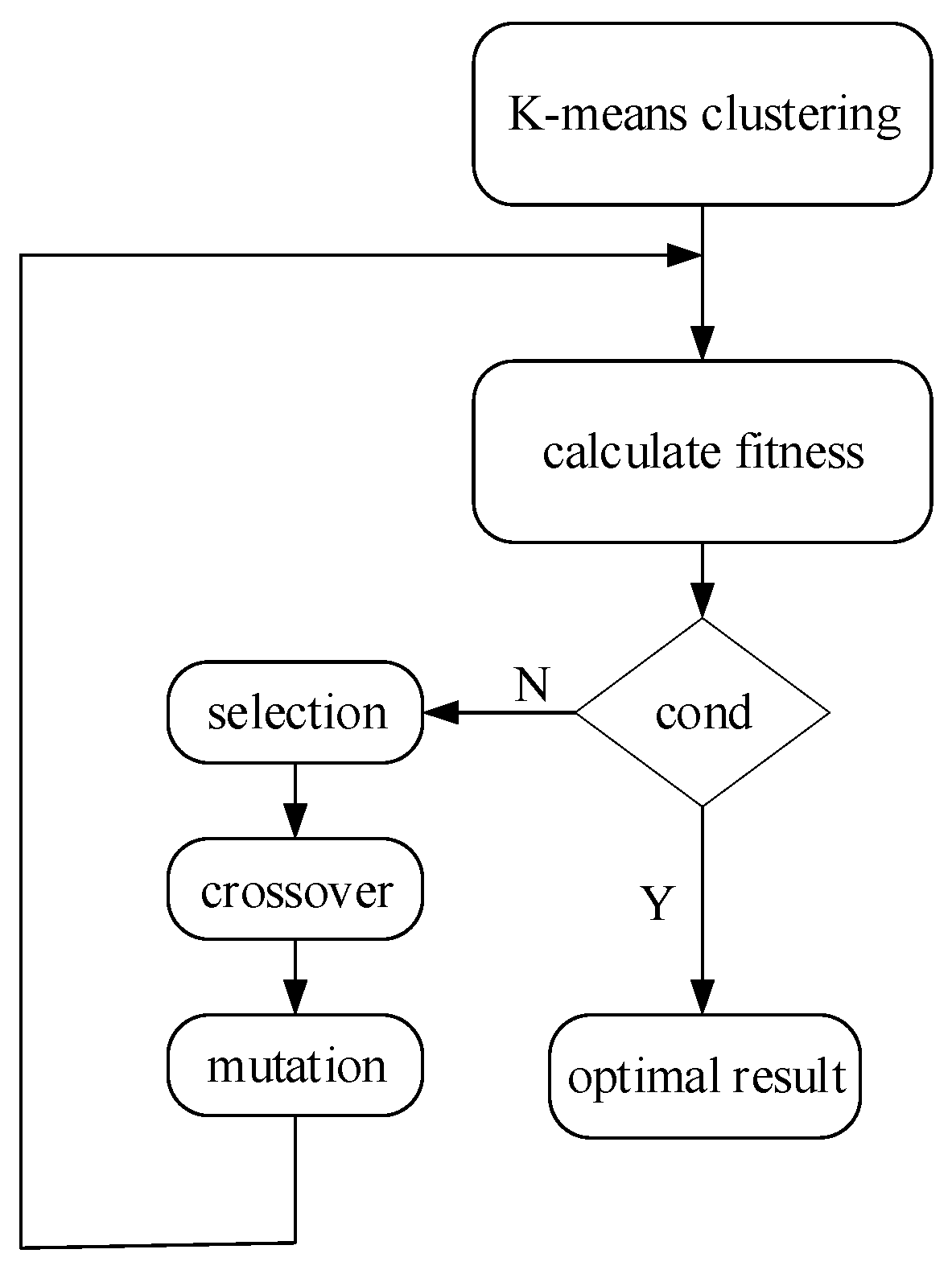
The Anchorage value is an important parameter used to predict the position and size of the object in the target detection algorithm. It is necessary to comprehensively consider the target size distribution, the nature of the training dataset, and other factors to obtain the optimal Anchorage value. In the YOLOv3 and YOLOv3-SPP network structure, there are nine prior boxes with different sizes which are divided into three groups according to the target size to detect small-, medium-, and large-size targets. According to the nature of the dataset in this paper, the size of the original prior box is no longer applicable, and it is necessary to obtain the size of the prior box suitable for this paper. In order to obtain an Anchorage value which is more suitable for target detection, the K-means [19,20] clustering algorithm and genetic algorithm [21] are used to calculate the Anchorage value by mutating the result of the K-means clustering. Among them, the Euclidean distance used in K-means clustering is changed in a distance-based way so that we can cluster to a more appropriate Anchorage value. The method of the abovementioned optimization process is as follows: first, the K-means clustering algorithm with the IoU as the metric of nine random anchors is optimized, and the fitness and the optimal threshold of the bpr (best possible recall) are calculated. The main parameters are bpr, mutation iteration times and fitness function parameters. Through many experiments, it is verified that the prior frame is the best when bpr is set to 0.98, and the best result comes if bpr > 0.98. If bpr < 0.98, GA (Genetic Algorithm) is used for iterative optimization. The number of variation iterations is set to 1000, and the fitness function parameter is a weighted combination of AP_0.5 and AP_0.5-0.9, with a weight ratio of 10% and 90% respectively. This paper mainly considers the gap between the width and height of 9 anchors and gt (ground truth) boxes when calculating bpr, that is, bpr selects the average value of width-height ratio for all gt boxes to meet the highest matching degree of threshold, of which threshold is the set threshold of width-height ratio and the ratio of length to width of gt box to anchor is

\frac{w_{g t}}{w_{a n}}

and

\frac{h_{g t}}{h_{a n}}

, and the value may be greater than 1 or less than 1. The author takes the reciprocal method to make the threshold less than or equal to 1). The algorithm is shown in Figure 5.

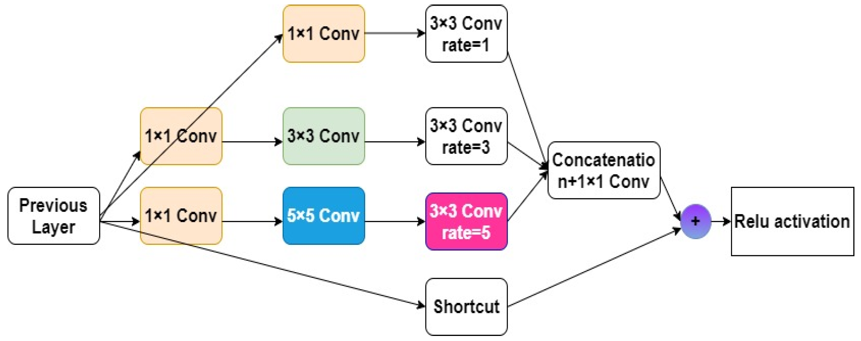
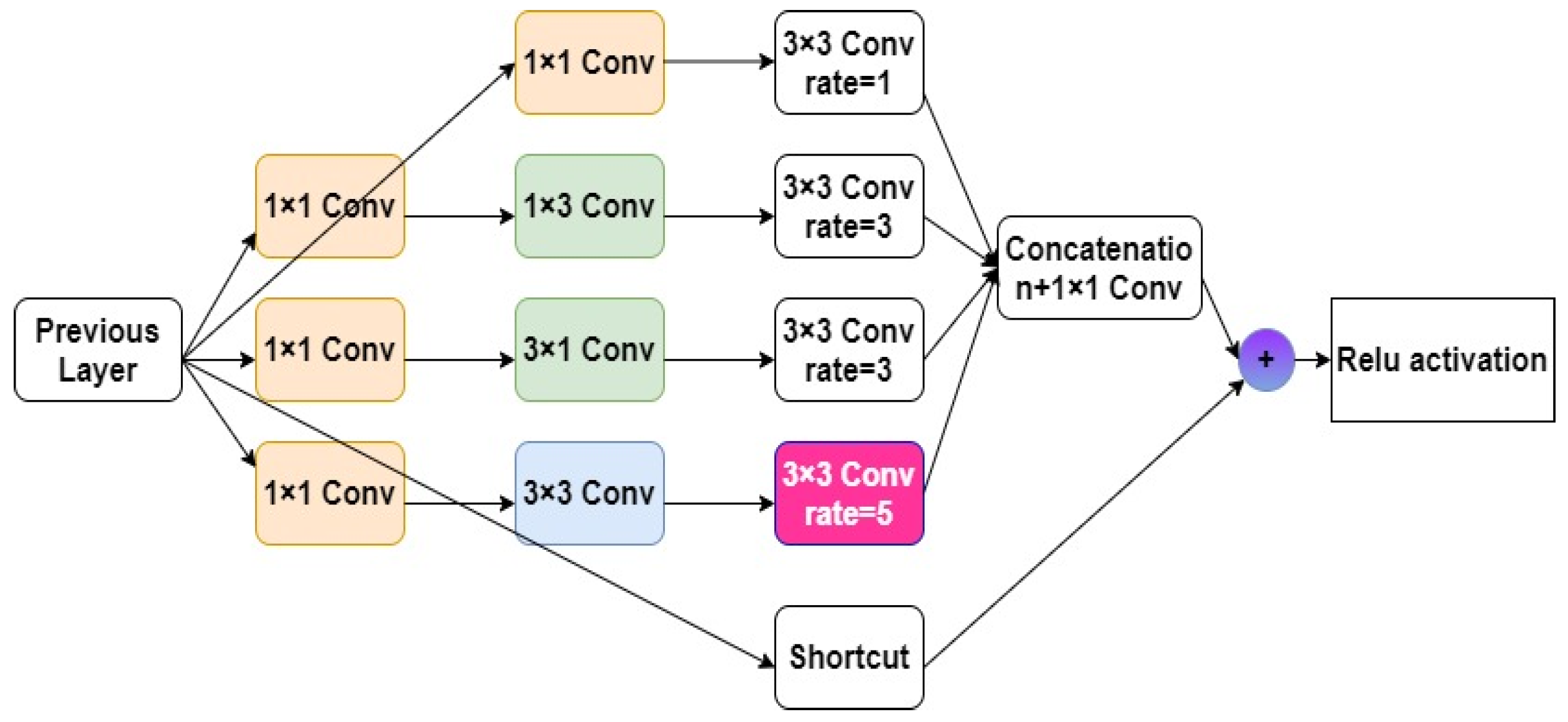
3.2.2. RFB and RFB-s Modules

RFB is a convolution neural network module composed of multi-layer convolution, an attention mechanism, and the ReLU activation function which is used to enhance the target detection algorithm's ability to perceive the target object and improve the detection accuracy. The main characteristics are as follows: (1) the RFB module contains several different convolution layers, each of which have a different convolution kernel size and convolution step length, so they can decipher the characteristics from a different visual field. (2) The attention mechanism is introduced to learn the importance of the features adaptively. (3) The void convolution layer is then introduced to enlarge the receptive field of the model. A different expansion factors rate is used in the RFB structure to represent the parameters of the cavity convolution layer. In the hollow convolution layer, there will be a certain interval between the elements in the convolution core, which is the expansion factor rate. The expansion factor rate represents the distance between the elements in the convolution core, which controls the size of the receptive field of the convolution layer. Specifically, if the size of the input characteristic graph of a convolution layer is HxW, the size of the convolution kernel is KxK, and the expansion factor rate is r, so the receptive field size of the convolution layer is:

(K + (K - 1) \times (r - 1)) \times (K + (K - 1) \times (r - 1))

(6)

It can be seen from the above formula that by adjusting the size of the expansion factor rate, the receptive field of the convolution layer can be changed without changing the size of the convolution core, thus learning the characteristics of different scales. The RFB structure is shown in Figure 6.

The RFB-s module is an improved module which adds a short connection and batch normalization operation to the RFB module. Short connections can make the model easier to train and optimize, avoiding the problems of gradient disappearance and gradient explosion. Batch normalization can accelerate the convergence of the model and improve the robustness of the model. The main advantage of the RFB-s module is that it can improve the detection speed and accuracy, and it is easier to train and optimize than the RFB module. Compared with RFB, RFB-s has two main improvements: (1) replacing the 5 × 5 convolution layer with a 3 × 3 convolution layer, and (2) replacing the 3 × 3 convolution layer with a 1 × 3 convolution layer and a 3 × 1 convolution layer. In order to reduce the amount of calculation and improve the speed and accuracy, this paper uses the RFB-s module to improve the YOLOv3-SPP, and its structure is shown in Figure 7.

3.2.3. Introduce EIoU Loss Function

The loss function used by YOLOv3-SPP is the same as YOLOv3, in which the bounding box position loss function IoU is used to measure the distance between the predicted bounding box and the real box, and this is calculated according to the center point coordinates and the width and height between the two boxes. The formula is as follows:

I o U = \frac{| A \cap B |}{| A \cup B |}

(7)

In the formula, A is the target prediction box and B is the real box.

In this paper, the EIOU loss function is introduced, and the calculation formula is as follows:

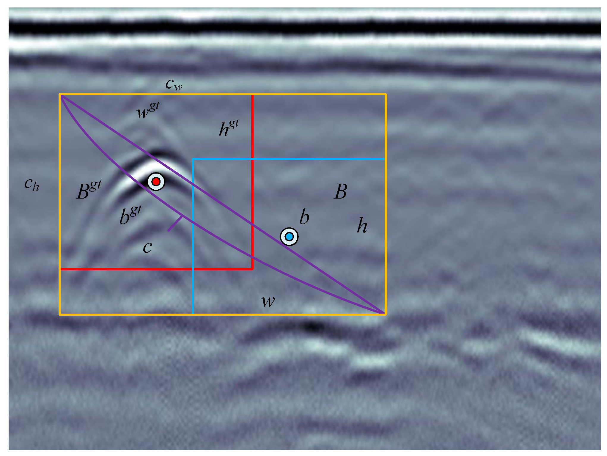
\begin{array}{l} L_{E I o U} (B, B^{g t}) = L_{I o U} + L_{d i s} + L_{a s p} \\ = 1 - I o U + \frac{ρ^{2} (b, b^{g t})}{c^{2}} + \frac{ρ^{2} (w, w^{g t})}{c_{w}^{2}} + \frac{ρ^{2} (h, h^{g t})}{c_{h}^{2}} \end{array}

(8)

The formula includes overlap loss, center distance loss, and width–height loss. The algorithm takes the aspect ratio apart on the basis of CIoU [22] and considers the width–height loss to minimize the width and height difference between the target box and the prediction box, so even if the size difference between the predicted boundary box and the real boundary box is large, the value of the EIoU can remain stable and accelerate convergence, in which the IoU is the ratio of the intersecting area of the prediction box and the target box to the merged area. As shown in Figure 8,

B, B^{g t}

represents the prediction box and the real box,

b, b^{g t}

represents the coordinates of the center point of the prediction box and the real box,

ρ (b, b^{g t})

represents the Euclidean distance between the two,

w, w^{g t}

and

h, h^{g t}

are the width and height of the prediction box and the real box,

c

is the diagonal length of the smallest circumscribed rectangle that can include both the prediction box and the real box, and

c_{w}, c_{h}

is the width and height of the minimum bounding box that can cover both boxes.

3.3 Model Evaluation Index

The YOLO series is used for target recognition using the cross-entropy loss function (cross-entropy loss), L, AP, mean average precision (mAP), and the detection rate FPS.

The cross-entropy loss function can measure the difference between the real value and the predicted value. The smaller the value is, the better the prediction effect of the model is. The formula is as follows:

L = - [\sum_{j = 1}^{N} x^{j} \ln ({\overset{⌢}{x}}^{j}) + (1 - x^{j}) \ln (1 - {\overset{⌢}{x}}^{j})]

(9)

In Formula (9), N is the total number of samples, which is expressed as the true value and predicted value of the j th sample.

AP is defined as the area under the curve of precision P and recall R, and the calculation formulas of the P, R, and AP are:

P = \frac{T_{P}}{T_{P} + F_{P}} \times 100 %

(10)

R = \frac{T_{P}}{T_{P} + F_{N}} \times 100 %

(11)

A P = \int_{0}^{1} P (R) d R

(12)

In the formula,

T_{P}

is the number of samples correctly identified,

F_{P}

is the number of samples mis-detected, and

F_{N}

is the number of samples missed by the model.

The mean AP values of N different categories are calculated, and the mean average precision (mAP) is obtained. As shown in Formula (13), the higher the mean average precision (mAP) value, the better the performance of the model.

m A_{P} = \frac{\sum A_{P c l a s s e s}}{N_{c l a s s e s}} \times 100 %

(13)

In the formula,

\sum A_{P c l a s s e s}

is the sum of the average precision values of each category, and

N_{c l a s s e s}

is the sum of the four categories.

In the application of ground-penetrating radar, if the target can be identified in a short time, preventive and remedial measures can be taken in advance. Therefore, the detection rate is also one of the indicators to measure the pros and cons of the model. The detection rate is defined as FPS, which represents the number of images processed by the model network per second. The formula is:

F P S = n / t

(14)

In Formula (14), n is the total number of frames processed, and t is the time used for corresponding the processing.

4. Analysis of Experimental Results

4.1. Experimental Environment

The network models proposed in this paper are implemented on the publicly available artificial neural network library and Tensor Flow framework. The experimental environment is configured with GPU: NVIDIA GeForce RTX 3060Ti, CPU: Intel(R) Core(TM) i7-10700F CPU @ 2.90GHz, and 64G RAM.

4.2. Model Parameter Setting and Training

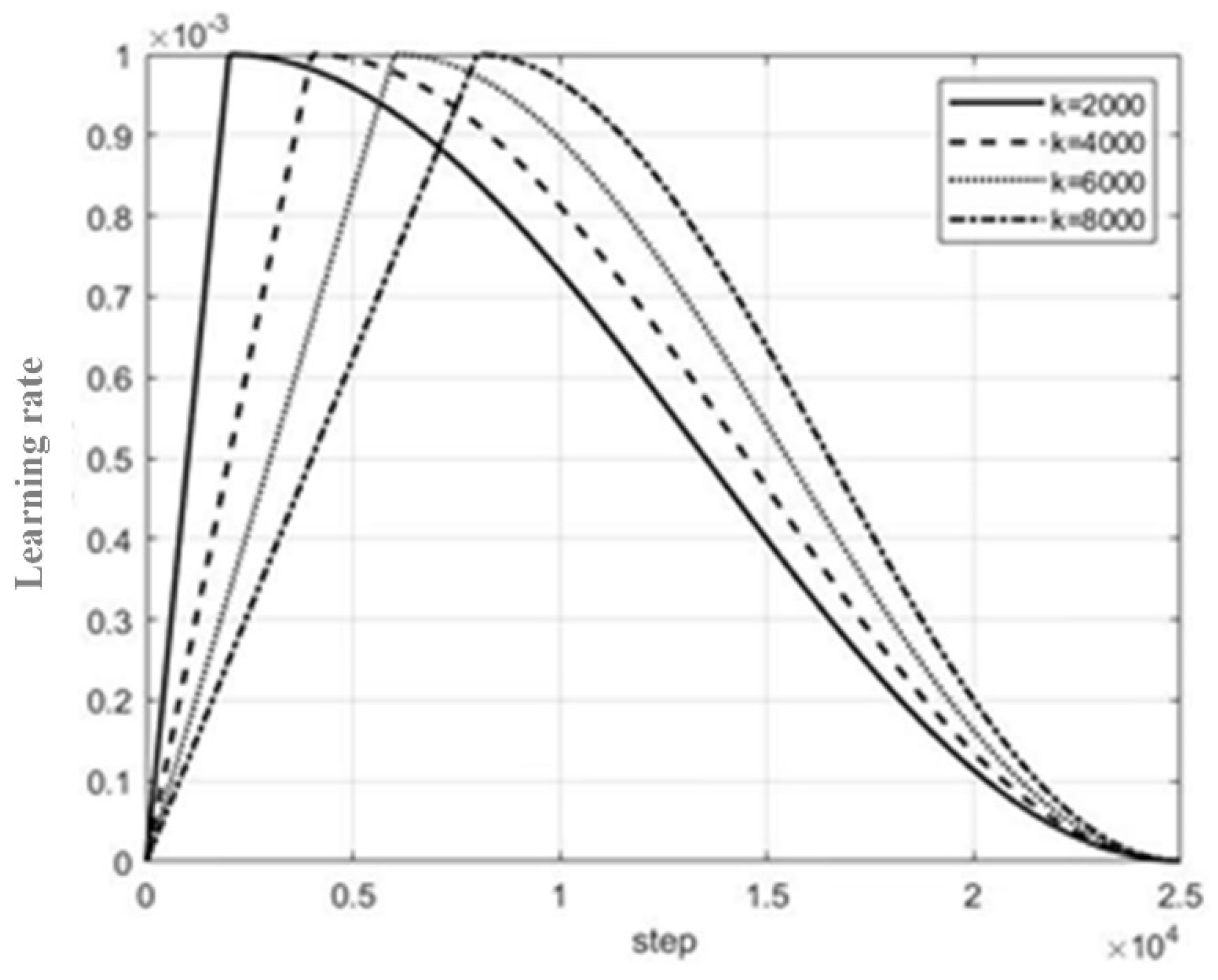
The dataset contains 2000 pictures of 2 kinds of simulation data and 2000 pictures of 3 kinds of real data. The two kinds of labels of simulation data are crack_S and pipe_S, there are no target classes and no tags in the real data, and the other two kinds of labels are crack and pipe. The training set has 3000 pictures, the test set has 1000 pictures, the batch_size in the network setting is 8, that is, 8 pictures are sent to the network for each batch of training, the initial learning rate lr is set to 0.001, the optimizer is set to 60, and the maximum number of iterations is 22500. The training method adopts the method of learning rate preheating; the learning rate increases linearly at first, but when the training times reaches 2000, the learning rate decreases as a cosine function. At the initial stage of training, the learning rate is larger, the convergence speed of the model is faster, and it tends to be stable, while in the later stage, the learning rate is small, which helps the model to converge and gradually approach the best point. The method of transfer learning is used to train the model. The learning rate transformation curve is shown in Figure 9, where the parameter k represents the number of training step required for the learning rate to reach its peak.

4.3. Ablation Experiments

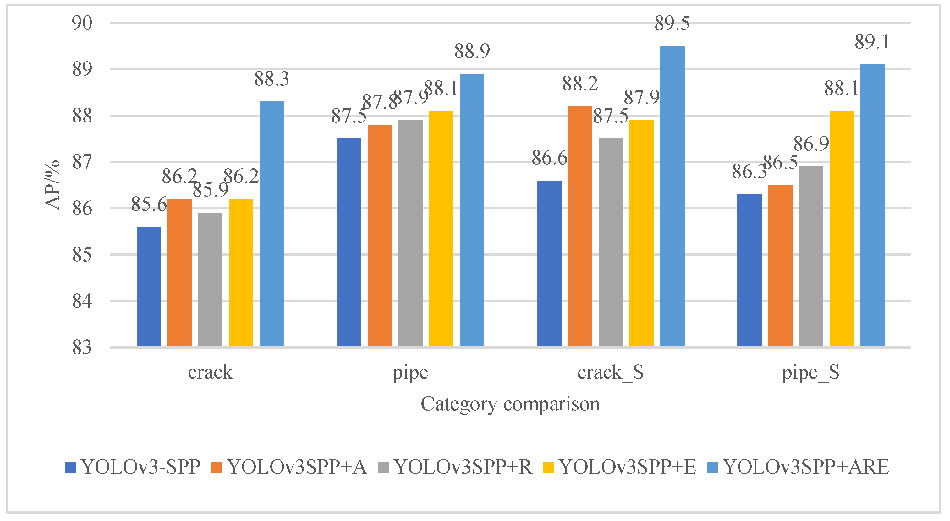
In order to verify the influence of the improved part of the optimization on the performance of the GPR echo image recognition model, we used the improved model based on the YOLOv3-SPP network structure (YOLOv3SPP+A), the improved model using only the RFB-s module (YOLOv3SPP+R), the improved model using the EIoU loss function (YOLOv3SPP+E), and the final improved model (YOLOv3SPP+ARE). The experimental results are shown in Table 1 and Figure 10.

From the data in Table 1 and Figure 10, we can see that in the echo target recognition model with optimized Anchorage values, the four categories of AP increased by 0.6, 0.3, 1.6, and 0.2 percentage points, respectively, and mAP increased by 0.7 percentage points, indicating that re-clustering Anchorage values can effectively improve the accuracy of the model. With the addition of the RFB-s module, although the recognition rate of the model decreased, the AP of the four categories increased by 0.3, 0.4, 0.9, and 0.6 percentage points, and the mAP increased by 0.6 percentage points. After introducing the EIoU loss function, the AP of the four categories identified by the model increased by 0.6, 0.6, 1.3, and 1.8 percentage points, and the mAP increased by 1.1 percentage points. With the introduction of the above three improvement strategies, the AP of the four categories increased by 2.7, 1.4, 2.9, and 2.8 percentage points, and the mAP increased by 2.5 percentage points. The experimental results show that the introduction of the above three improved strategies effectively improved the accuracy of the GPR echo target recognition.

4.4. Comparative Analysis of Models

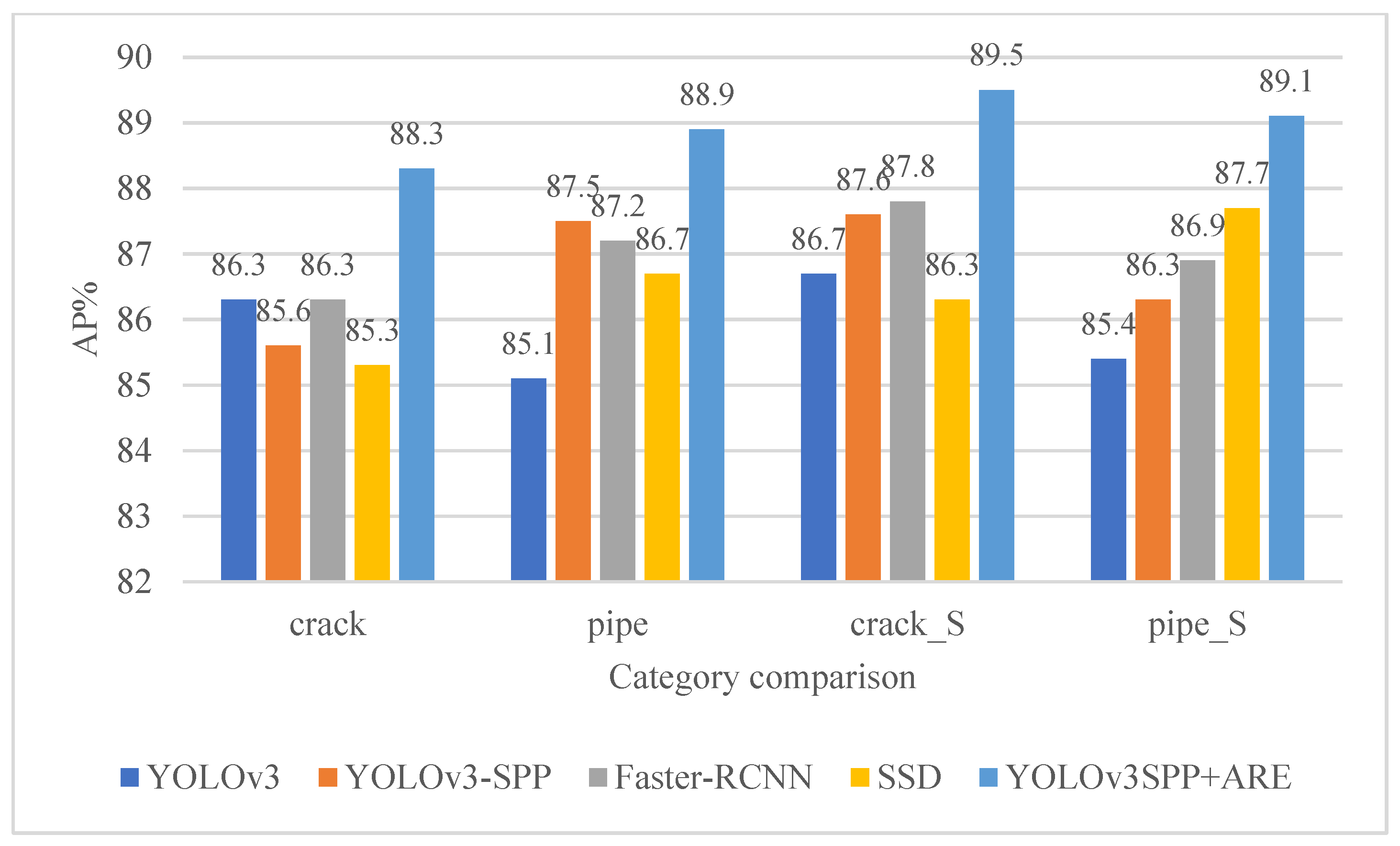
By comparing with other disclosed deep learning models, the comprehensive performance of the improved YOLOv3-SPP can be compared, including YOLOv3, YOLOv3-SPP, Faster R-CNN [23], and SSD (Single Shot MultiBox Detector) [24]. The performance of the algorithm proposed in this paper is evaluated by comprehensively comparing the performance of several models on the test set. The experimental results are shown in Table 2 and Figure 11.

According to the data in Table 2 and Figure 11, the AP of this algorithm is higher than that of each model in the four categories, which is 2, 4.8, 3.2, and 3.7 percentage points higher than that of the other four models with the highest AP. The mAP of this algorithm is 89.0%, which is 3.1, 2.2, 1.9, and 2.5 percentage points higher than the other four algorithm models YOLOv3, YOLOv3-SPP, Faster R-CNN, and SSD (Single Shot MultiBox Detector), respectively. Although the detection rate of the algorithm proposed in this paper is not the best, considering that the detection accuracy is improved and the detection rate is similar to other models, it can be considered that the improved YOLOv3-SPP algorithm model not only achieves a higher recognition accuracy but it also takes into account the detection rate, and has the best effect on GPR echo target recognition.

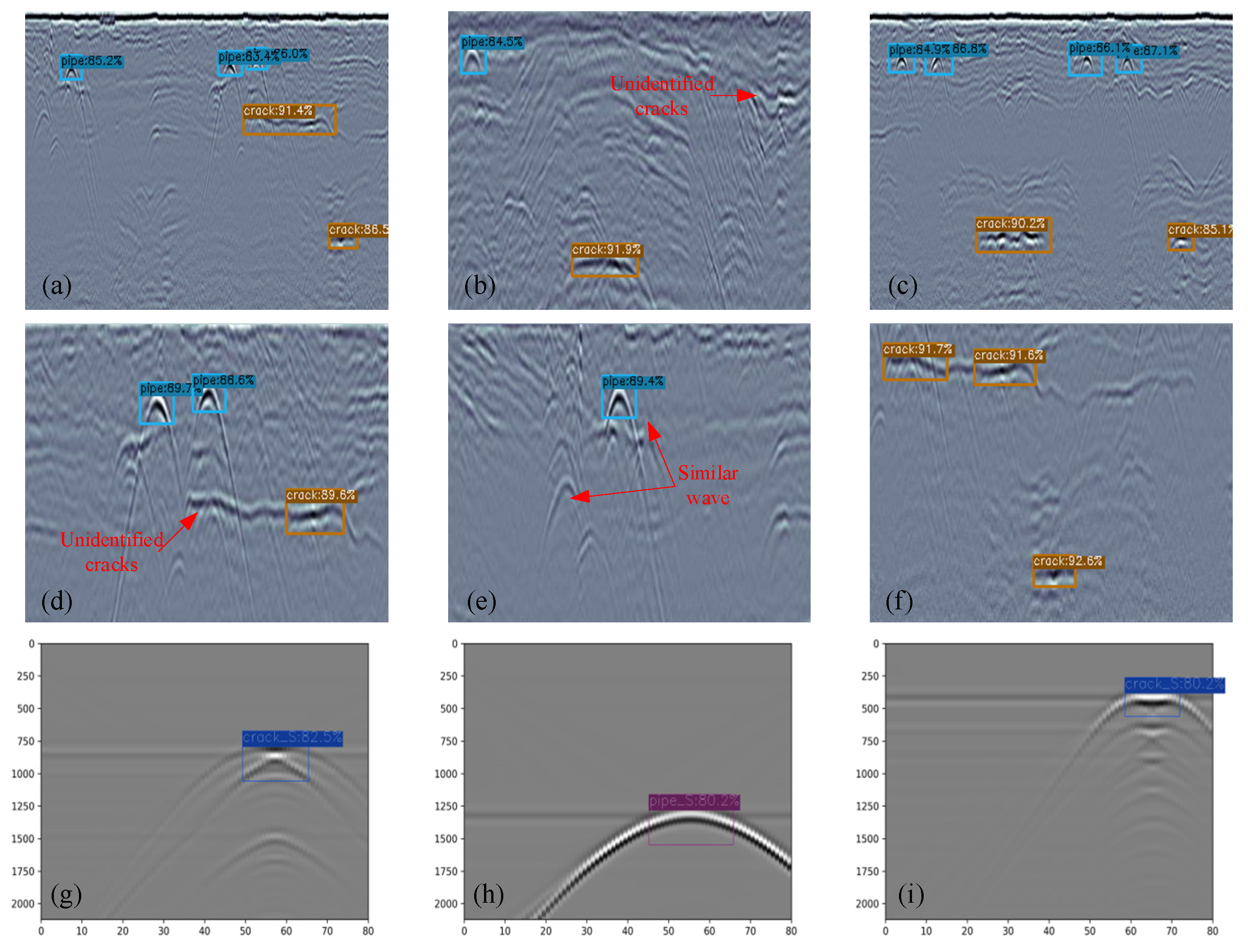
The prediction effect of the improved model is shown in Figure 12 after recognizing the simulated and real GPR images. In figure (a)-(d), the model simultaneously detects the echo characteristics of multiple pipelines and diseases in the GPR map. The echo intensity of the diseases in figure (b) and figure (d) is weak and cannot be identified. There are similar echo characteristics in figure (e) which will not be mistakenly detected. The model in figure (f) can identify the corresponding crack diseases, but it will not be mistakenly detected for some interlayer defects with a weak echo intensity. Figure (g)-(I) is the single target of the disease and pipeline in the simulation data image, which can be identified accurately by the model. The improved YOLOv3-SPP model can identify four kinds of targets and can identify multiple targets in the echo image of the real data, including the location of random targets, and output the confidence and target category of the prediction box.

5. Conclusion

Aiming to solve the problem of target recognition in GPR echo images, this paper proposed an improved strategy based on the YOLOv3-SPP algorithm, which optimizes the Anchorage value, adds the RFB-s module, and introduces the EIoU loss function, which improves the recognition accuracy while maintaining the detection rate. A GPR image dataset simulated by the software was used to preprocess the removal of direct waves, and the processed data and road datasets were used for training and testing. The AP and mAP of the four categories identified by the proposed algorithm model reached 88.3%, 88.9%, 89.5%, 89.1%, and 89.0%, respectively, which were higher than YOLOv3-SPP. Additionally, through the setting comparison experiment, the effectiveness and accuracy of the proposed algorithm were verified. The experimental results show that the comprehensive performance of the algorithm proposed in this paper is better, and it has been proved that the algorithm model can effectively identify and locate the targets in the GPR echo image, which provides a feasible reference for the future of GPR echo image recognition direction.

References

Liu, H.; Huang, Z.G.; Yue, Y.P.; Cui, J.; Hu, Q.F. Characteristics Analysis of Ground Penetrating Radar Signals for Ground water Pipe Leakage Environment. JOURNAL OF ELECTRONICS & INFORMATION TECHNOLOGY 2022, 44, 1257–1264. [Google Scholar]
Stryk, J.; Matula, R.; Pospisil, K.; Derobert, X.; Simonin, J.M.; Alani, A.M. Comparative measurements of ground penetrating radars used for road and bridge diagnostics in the Czech Republic and France. CONSTR BUILD MATER 2017, 154, 1199–1206. [Google Scholar] [CrossRef]
Harseno, R.W.; Lee, S.J.; Kee, S.H.; Kim, S. Evaluation of Air-Cavities behind Concrete Tunnel Linings Using GPR Measurements. REMOTE SENS-BASEL 2022, 14. [Google Scholar] [CrossRef]
Amran, T.; Ismail, M.P.; Ismail, M.A.; Amin, M.; Ahmad, M.R.; Basri, N. , GPR application on construction foundation study. In GLOBAL CONGRESS ON CONSTRUCTION, MATERIAL AND STRUCTURAL ENGINEERING 2017 (GCOMSE2017), AbdRahman, N.; Khalid, F. S.; Othman, N. H.; Ghing, T. Y.; Yong, L. Y.; Ali, N., ^Eds. Global Congress on Construction, Material and Structural Engineering (GCoMSE), 2017; Vol. 271.
Joshaghani, A.; Shokrabadi, M. Ground penetrating radar (GPR) applications in concrete pavements. INT J PAVEMENT ENG 2022, 23, 4504–4531. [Google Scholar] [CrossRef]
Thomas, S.B.; Roy, L.P. Signal processing for coal layer thickness estimation using high-resolution time delay estimation methods. IET SCI MEAS TECHNOL 2017, 11, 1022–1031. [Google Scholar] [CrossRef]
J. , P.; C., L.B.; Y., W.; M., S. Time-Delay Estimation Using Ground-Penetrating Radar With a Support Vector Regression-Based Linear Prediction Method. IEEE T GEOSCI REMOTE 2018, 56, 2833–2840. [Google Scholar] [CrossRef]
Redmon, J.; Farhadi, A. ; IEEE, YOLO9000: Better, Faster, Stronger. In 30TH IEEE CONFERENCE ON COMPUTER VISION AND PATTERN RECOGNITION (CVPR 2017), 30th IEEE/CVF Conference on Computer Vision and Pattern Recognition (CVPR), 2017; pp 6517-6525.
Redmon, J.; Farhadi, A. YOLOv3: An Incremental Improvement. arXiv e-prints 2018. [Google Scholar]
Redmon, J.; Divvala, S.; Girshick, R.; Farhadi, A. ; IEEE, You Only Look Once: Unified, Real-Time Object Detection. In 2016 IEEE CONFERENCE ON COMPUTER VISION AND PATTERN RECOGNITION (CVPR), 2016 IEEE Conference on Computer Vision and Pattern Recognition (CVPR), 2016; pp 779-788.
Balcioglu, Y.S.; Sezen, B.; Gok, M.S.; Tunca, S. IMAGE PROCESSING WITH DEEP LEARNING: SURFACE DEFECT DETECTION OF METAL GEARS THROUGH DEEP LEARNING. MATER EVAL 2022, 80, 44–53. [Google Scholar] [CrossRef]
Han, Y.C.; Wang, J.; Lu, L. ; IEEE, A Typical Remote Sensing object detection Method Based on YOLOv3. In 2019 4TH INTERNATIONAL CONFERENCE ON MECHANICAL, CONTROL AND COMPUTER ENGINEERING (ICMCCE 2019), 4th International Conference on Mechanical, Control and Computer Engineering (ICMCCE), 2019; pp 520-523.
Yang, Z.L. Intelligent Recognition of Traffic Signs Based on Improved YOLO v3 Algorithm. MOB INF SYST 2022, 2022. [Google Scholar] [CrossRef]
T., Y.L.; P., D.; R., G.; K., H.; B., H.; S., B. In Feature Pyramid Networks for Object Detection, 2017 IEEE Conference on Computer Vision and Pattern Recognition (CVPR), 21-26 July 2017; pp. 936–944.
K. , H.; X., Z.; S., R.; J., S. Spatial Pyramid Pooling in Deep Convolutional Networks for Visual Recognition. IEEE T PATTERN ANAL 2015, 37, 1904–1916. [Google Scholar] [CrossRef] [PubMed]
Liu, S.; Huang, D.; Wang, Y. In Receptive Field Block Net for Accurate and Fast Object Detection, Cham, 2018, 2018; Ferrari, V.; Hebert, M.; Sminchisescu, C.; Weiss, Y., Eds. Springer International Publishing: Cham, 2018; pp. 404-419.
Zhang, Y.F.; Ren, W.; Zhang, Z.; Jia, Z.; Wang, L.; Tan, T. Focal and Efficient IOU Loss for Accurate Bounding Box Regression. 2021.
Zhao Di，Ye Shengbo，Zhou Bin. Ground penetrating radar anomaly detection based on convolution Grad-CAM. Electronic Measurement Technology 2020, 43, 113–118. [Google Scholar]
Aggarwal, S.; Singh, P. Cuckoo, Bat and Krill Herd based k-means plus plus clustering algorithms. CLUSTER COMPUT 2019, 22, 14169–14180. [Google Scholar] [CrossRef]
Sinaga, K.P.; Yang, M.S. Unsupervised K-Means Clustering Algorithm. IEEE ACCESS 2020, 8, 80716–80727. [Google Scholar] [CrossRef]
J. , E.; R., G.; B., U.; R., G. Optimization of Sparse Time-Modulated Array by Genetic Algorithm for Radar Applications. IEEE ANTENN WIREL PR 2014, 13, 161–164. [Google Scholar] [CrossRef]
Zheng, Z.; Wang, P.; Liu, W.; Li, J.; Ye, R.; Ren, D. Distance-IoU Loss: Faster and Better Learning for Bounding Box Regression. arXiv 2019. [Google Scholar] [CrossRef]
Ren, S.; He, K.; Girshick, R.; Sun, J. Faster R-CNN: Towards Real-Time Object Detection with Region Proposal Networks. IEEE Transactions on Pattern Analysis & Machine Intelligence 2017, 39, 1137–1149. [Google Scholar]
Berg, A.C.; Fu, C.Y.; Szegedy, C.; Anguelov, D.; Erhan, D.; Reed, S.; Liu, W. SSD: Single Shot MultiBox Detector. 2015.

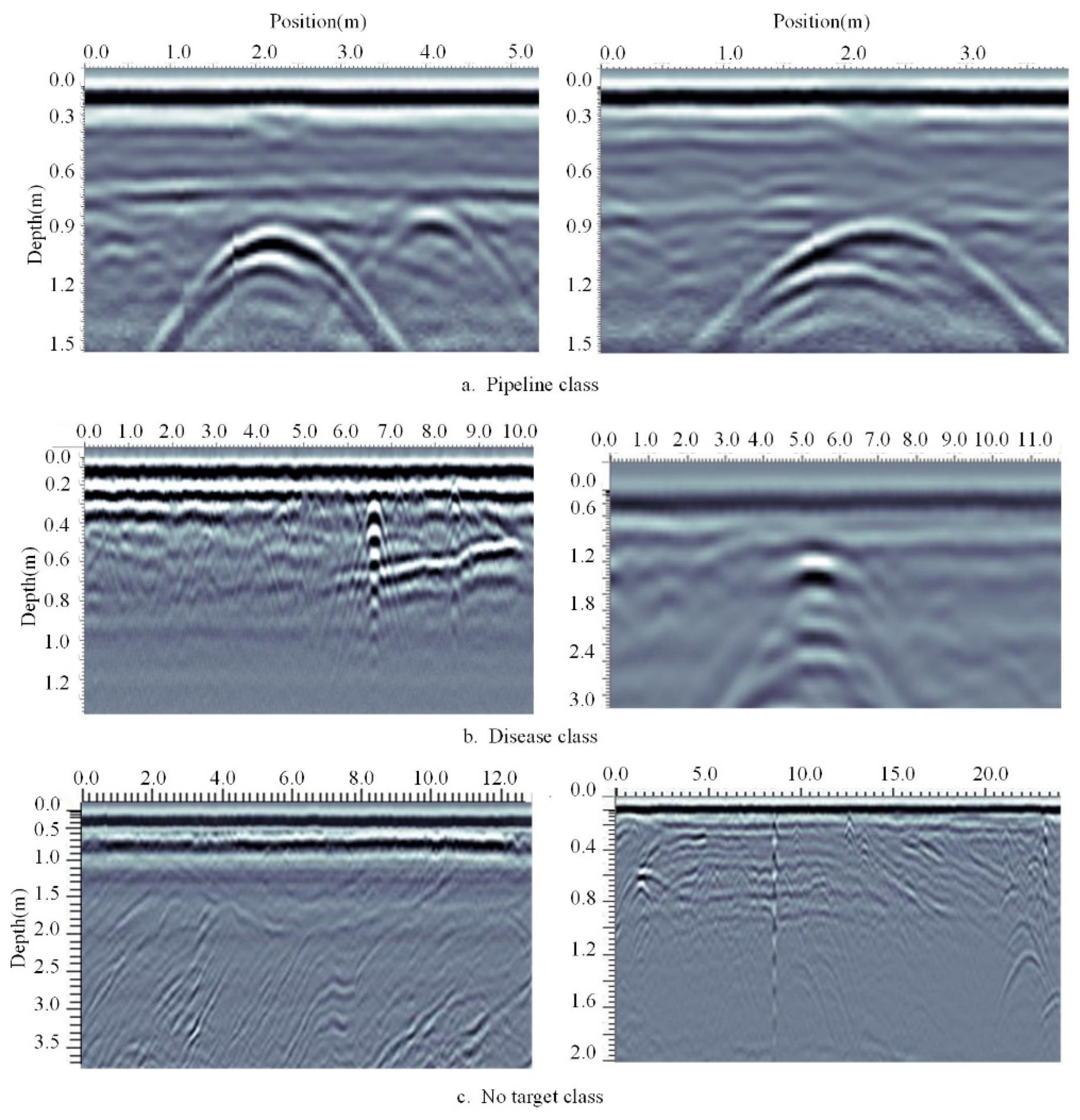
Figure 1. Three ground-penetrating radar echo images.

Figure 2. B-scan original images (including direct waves).

Figure 3. B-scan image after removing direct waves.

Figure 4. Structure of the improved YOLOv3-SPP network.

Figure 5. Algorithm flow chart.

Figure 6. RFB module structure diagram.

Figure 7. RFB-s module structure diagram.

Figure 8. EIoU loss of frame regression.

Figure 9. Learning rate change curve.

Figure 10. Comparison of AP in ablation experiment.

Figure 11. AP comparison diagrams of 4 categories.

Figure 12. Recognition effect picture.

Table 1. Results of ablation experiments.

Models	mAP/%	FPS/(frame/s)
YOLOv3-SPP	86.5	67
YOLOv3SPP+A	87.2	67
YOLOv3SPP+R	87.1	60
YOLOv3SPP+E	87.6	67
YOLOv3SPP+ARE	89.0	60

Table 2. mAP and FPS of each model.

Models	mAP/%	FPS/(frame/s)
YOLOv3	85.9	72
YOLOv3-SPP	86.8	67
Faster R-CNN	87.1	17
SSD	86.5	40
YOLOv3SPP+ARE	89.0	60

Disclaimer/Publisher’s Note: The statements, opinions and data contained in all publications are solely those of the individual author(s) and contributor(s) and not of MDPI and/or the editor(s). MDPI and/or the editor(s) disclaim responsibility for any injury to people or property resulting from any ideas, methods, instructions or products referred to in the content.

© 2023 by the authors. Licensee MDPI, Basel, Switzerland. This article is an open access article distributed under the terms and conditions of the Creative Commons Attribution (CC BY) license (http://creativecommons.org/licenses/by/4.0/).

Copyright: This open access article is published under a Creative Commons CC BY 4.0 license, which permit the free download, distribution, and reuse, provided that the author and preprint are cited in any reuse.

MDPI Initiatives

Important Links

Choose an area of interest and we will send you notifications of new preprints at your preferred frequency.

Disclaimer

GPR Target Recognition Based on Improved YOLOv3-SPP

Abstract

1. Introduction

2. Introduction and Preprocessing of Dataset

2.1 Brief Introduction of Ground-Penetrating Radar

2.2 Experimental Real Data

2.3 GPRMAX Simulation Data

3. Introduction and Improvement of YOLOv3-SPP Algorithm

3.1 YOLOv3-SPP

3.2 Improved YOLOv3-SPP

3.2.1. Optimize the Anchorage Value

3.2.2. RFB and RFB-s Modules

3.2.3. Introduce EIoU Loss Function

3.3 Model Evaluation Index

4. Analysis of Experimental Results

4.1. Experimental Environment

4.2. Model Parameter Setting and Training

4.3. Ablation Experiments

4.4. Comparative Analysis of Models

5. Conclusion

References

MDPI Initiatives

Important Links

Subscribe