Collision Entropy Estimation in a One-Line Formula

Preprint

Article

Collision Entropy Estimation in a One-Line Formula

Altmetrics

Downloads

165

Views

Comments

Alessandro Gecchele^*

This version is not peer-reviewed

Submitted:

23 May 2023

Posted:

24 May 2023

You are already at the latest version

Alerts

Abstract

We address the unsolved question of how best to estimate the collision entropy, also called quadratic or second order Rényi entropy. Integer-order Rényi entropies are synthetic indices useful for the characterization of probability distributions. In recent decades, numerous studies have been conducted to arrive at their valid estimates starting from experimental data, so to derive suitable classification methods for the underlying processes, but optimal solutions have not been reached yet. Limited to the estimation of collision entropy, a one-line formula is presented here. The results of some specific Monte Carlo experiments give evidence of the validity of this estimator even for the very low densities of the data spread in high-dimensional sample spaces. The method strengths are unbiased consistency, generality and minimum computational cost.

Keywords:

Subject: Physical Sciences - Mathematical Physics

1. Introduction

The information theory indices belonging to the parametric family of Rényi entropies are able to express, each with a different weight, the information content of a discrete probability distribution (

D P D

) [1]. Typical members of this family are, for example, Shannon entropy, collision entropy and min-entropy. These indices can also be used to classify the output of experimental processes studied in any branch of the applied sciences, provided their reduction to pseudostationary discrete-state processes and then in the form of

D P D

s. Since usually, during the experiments, only brief realizations can be obtained from the process under investigation, and since the realizations give rise to relative frequency distributions (

R F D

s) and not to

D P D

s, then these indices, being based on probabilities, have to be estimated through the elaboration of the few available data. In this regard, the methods for the estimation of Rényi entropies are of two kinds: 1) those that first aim to estimate the probability distribution from the relative frequencies and then plug the estimated probabilities into the formulas of the entropies and 2) those that circumvent the still-open problem of the estimation of the probabilities and aim to estimate the entropy indices through the application of other elaborations to the data. Despite the numerous studies carried out in the last decades (e.g., [2,3,4,5,6,7,8,9,10,11,12,13,14,15,16,17,18,19,20,21,22,23,24,25,26,27,28,29,30,31,32,33,34]), definitive and universally accepted results for these issues have not been found yet. Moreover, this persistent lack of satisfactory solutions for the estimation of the indices belonging to the Rényi family (and for the estimation of their more rapidly converging derived quantities called Rényi entropy rates) has prompted, as a side effect, an anomalous proliferation of other similar indices conceived in many different ways (e.g. [35,36,37]), but all having the same purpose of classifying data with a nonparametric approach. An overview of this peculiar situation, which, by the way, Shannon in 1956 [38] recommended to avoid, can be found in [39], where Ribeiro et al. collected and described a "galaxy" of at least thirty indices somehow functionally equivalent to those of the family initially proposed by Rényi (and to their rates). Returning to the original question, Skorski ([40,41]) rightly pointed out that the estimation of those integer-order Rényi entropies that have a parameter value greater than one reduces to the estimation of the moments of a

D P D

. Our work just starts from this latter consideration and limits its investigation only to the case of the estimation of the second raw moment, which, in turn, allows the collision entropy to be estimated.

2. Theoretical Methods

2.1. Transforming a Discrete-State Stochastic Process into a DPD

Consider a discrete-state stochastic process (

D S P_{q}

) whose infinite values

\dots, x_{i - 1},

x_{i}, x_{i + 1}, \dots

belong to an alphabet A containing q ordered symbols. Let

Ω (q, d)

be a d-dimensional discrete sample space resulting from the Cartesian product d times of A

Ω (q, d) = \underset{d t i m e s}{\underset{︸}{A \times A \times . . . \times A}},

(1)

and let

n = q^{d}

be the cardinality of the sample space

Ω (q, d)

. Each elementary event

e_{k}

, with

k \in {1, 2, . . ., n}

, is uniquely identified by a vector with d coordinates (

x 1_{k}, x 2_{k}, . . ., x d_{k}

), with

x 1_{k}, x 2_{k}, . . ., x d_{k} \in A

. Following the procedure indicated by Shannon in [42] at pages 5 and 6, the infinite sequence of samples constituting the

D S P_{q}

can be transformed into occurrences

# (e_{k})

of the elementary events of

Ω (q, d)

by progressively considering all the d-grams taken from the samples as if they were the coordinates of the events and counting the number of times that each coordinate appears in the sequence. Then, according to the frequentist definition of probability, the final resulting

D P D

is expressible in set theory notation as

p {(Ω (q, d))}_{D S P_{q}} = \{p {(e_{k})}_{D S P_{q}} = \frac{# {(e_{k})}_{D S P_{q}}}{\sum_{k = 1}^{n} # {(e_{k})}_{D S P_{q}}} | e_{k} \in Ω (q, d)\} .

(2)

In the following, in the absence of ambiguity,

p {(Ω (q, d))}_{D S P_{q}}

—that is, a

D P D

obtained by elaborating the data of a

D S P_{q}

— will be indicated with the bold symbol

p

and one of its elements with

p_{k}

2.2. Integer-Order Rényi $α$ -Entropies as Synthetic Indices for the Characterization of $D P D$ s

In general, a

D P D

can be characterized by some indices, each of which can quantify the presence rate of a particular feature in the distribution. The parametric family of integer-order Rényi α-entropies is composed of synthetic indices suitable for the characterization of

D P D

s from the point of view of their informative content. According to [1] and imposing

α \in N^{+}

, they are defined as

\begin{matrix} α = 1 H_{1} (p) ≜ - \sum_{k = 1}^{n} p_{k} \log p_{k} \\ α \neq 1 H_{α} (p) ≜ \frac{1}{1 - α} \log (\sum_{k = 1}^{n} p_{k}^{α}) 0 \leq H_{α} (p) \leq \log n \\ α \to \infty H_{\infty} (p) ≜ - \log m a x {p} . \end{matrix}

(3)

The corresponding specific integer-order Rényi α-entropy of the

D P D

p

is then defined as

\begin{matrix} α = 1 η_{1} (p) ≜ \frac{H_{1} (p)}{\log n} = - \sum_{k = 1}^{n} p_{k} \log_{n} p_{k} \\ α \neq 1 η_{α} (p) ≜ \frac{H_{α} (p)}{\log n} = \frac{1}{1 - α} \log_{n} (\sum_{k = 1}^{n} p_{k}^{α}) 0 \leq η_{α} (p) \leq 1 \\ α \to \infty η_{\infty} (p) ≜ \frac{H_{\infty} (p)}{\log n} = - \log_{n} m a x {p} . \end{matrix}

(4)

Once the value of a specific entropy is known, it is always possible to retrieve the value of the corresponding plain entropy, expressed in a particular base b and for a particular cardinality n, using the following conversion formula:

H_{α} (p, b, n) ≜ η_{α} (p) {log}_{b} n .

(5)

Specific entropies are preferable to plain entropies because:

1: they are the result of a min-max normalization, that is obtained using the minimum and the maximum possible values of plain entropies (respectively 0 and $\log n$ );
2: they are formally independent from the number of ordered symbols q chosen for the quantization of the range of the output values of the process and independent from the cardinality of the sample space n; for this reason, they allow comparable values to be obtained, even for different distributions in different sample spaces;
3: they allow the doubt on the choice of the base for the logarithm present in the formula of entropies ( $2$ or $e$ or $10$ ) to be removed, thanks to the use of a variable base, depending on the cardinality of the considered sample space ( $n$ );

2.3. Rényi Entropy Rates

Unlike Rényi entropies, whose utility is mainly related to the classification of

D P D

s, Rényi entropy rates are important theoretical quantities useful for the characterization of

D S P_{q}

s [43,44]; they are defined as

H_{α}^{'} (D S P_{q}) ≜ lim_{d \to \infty} \frac{1}{d} H_{α} (p {(Ω (q, d))}_{D S P_{q}}) 0 \leq H_{α}^{'} (D S P_{q}) \leq \log q .

(6)

Moreover, it is known that, for strongly stationary

D S P_{q}

, any Rényi entropy rate converges to the same limit of a sequence of Cesaro means of conditional entropies:

H_{α}^{'} (D S P_{q}) = lim_{d \to \infty} H_{α} (p (A_{d}) | p (A_{1} \times A_{2} \times \dots \times A_{d - 1})) .

(7)

and, as conditional Rényi entropies preserve the chain rule [45,46,47], they can also be calculated as

H_{α}^{'} (D S P_{q}) = lim_{d \to \infty} [H_{α} (p {(Ω (q, d))}_{D S P_{q}}) - H_{α} (p {(Ω (q, d - 1))}_{D S P_{q}})] .

(8)

2.4. Specific Rényi Entropy Rate

Similarly to Formula (4), specific Rényi entropy rate is defined by the following min-max normalization:

\begin{matrix} η_{α}^{'} (D S P_{q}) = \frac{H_{α}^{'} (D S P_{q})}{\log q} = \\ = lim_{d \to \infty} \frac{[H_{α} (p {(Ω (q, d))}_{D S P_{q}}) - H_{α} (p {(Ω (q, d - 1))}_{D S P_{q}})]}{\log q} = \\ = lim_{d \to \infty} [d η_{α} (p {(Ω (q, d))}_{D S P_{q}}) - (d - 1) η_{α} (p {(Ω (q, d - 1))}_{D S P_{q}})], \end{matrix}

(9)

with

0 \leq η_{α}^{'} (D S P_{q}) \leq 1

2.5. Relationship between Specific Rényi Entropy Rate and Specific Rényi Entropy

In summary, the following relationship subsists:

η_{α}^{'} (D S P_{q}) = lim_{d \to \infty} η_{α} (p {(Ω (q, d))}_{D S P_{q}})

(10)

This means that, varying d, the specific Rényi entropy tends to the same value of the specific Rényi entropy rate, with the important difference being that the rate of convergence of the specific Rényi entropy rate is much faster than the rate of convergence of the specific Rényi entropy. For this reason, when possible, using the specific Rényi entropy rate is preferable to using the specific Rényi entropy.

3. Empirical Methods

3.1. Transforming a Realization into a Distribution of Relative Frequencies

For the practical cases, the theoretical procedure described in § Section 2.1 can be adapted according to the following procedure already presented with greater generality in [48] and in [49]: consider the N samples

x_{1}, x_{2}, \dots, x_{d}, x_{d + 1}, \dots, x_{N}

of a realization

r_{q}

extracted from a

D S P_{q}

. Each d-gram composed of d adjacent samples of

r_{q}

is interpreted as the occurrence of the elementary event of a d-dimensional sample space

Ω (q, d)

having just those values as vector components. For example, the first two d-grams taken from

r_{q}

(x_{1}, x_{2}, . . ., x_{d})

and

(x_{2}, x_{3}, . . ., x_{d + 1})

identify the first occurrences of two elementary events. The count of the occurrences of the events is performed for all the d-grams progressively identified in the sequence of the samples of

r_{q}

. Finally, the absolute frequency of every elementary event

# (e_{k})

is divided by the total number of occurrences (

L = \sum_{k = 1}^{n} # {(e_{k})}_{r_{q}} = N - d + 1

), yielding its relative frequency

f {(e_{k})}_{r_{q}}

. The final resulting

R F D

is expressible in set theory notation as

f {(Ω (q, d))}_{r_{q}} = \{f {(e_{k})}_{r_{q}} = \frac{# {(e_{k})}_{r_{q}}}{\sum_{k = 1}^{n} # {(e_{k})}_{r_{q}}} | e_{k} \in Ω (q, d)\}

(11)

In the following, in the absence of ambiguity, an RFD

f {(Ω (q, d))}_{r_{q}}

resulting from the insertion of the data of a realization in a sample space will be simply indicated with the bold symbol

f

and

f_{k}

indicates one of its elements.

3.2. Estimating the Second Raw Moment of a $D P D$

Preliminarily the

α^{t h}

-raw moment of a

D P D

p

and the

α^{t h}

-raw moment of a

R F D

f

are defined as

M_{α} (p) ≜ \sum_{k = 1}^{n} p_{k}^{α}, M_{α} (f) ≜ \sum_{k = 1}^{n} f_{k}^{α} \frac{1}{n^{α - 1}} \leq M_{α} (\cdot) \leq 1

(12)

Limited to the raw moments of Poissonian distributions, Grassberger in [2], Formula (8), and subsequently Schürmann after sixteen years in [12], Formula (6), reported the theoretically demonstrable, unique unbiased estimator, repeated in Formula (13):

\begin{matrix} {\hat{M_{α} (p)}}_{P o i s s o n} = {〈\sum_{k = 1}^{n} \hat{p_{k}^{α}}〉}_{r_{q}} = \sum_{k = 1}^{n} {〈\frac{1}{L^{α}} \frac{# {(e_{k})}_{r_{q}}!}{(# {(e_{k})}_{r_{q}} - α)!}〉}_{r_{q}} \\ \hat{p_{k}^{α}} : = 0 f o r # {(e_{k})}_{r_{q}} < α, \end{matrix}

(13)

where

< \cdot >_{r_{q}}

is the mean over the infinite number of realizations that can be taken from the underlying process. For the specific case of the estimation of the second raw moment, Formula (13) becomes:

\hat{M_{2} (p})_{P o i s s o n} = \sum_{k = 1}^{n} {〈\frac{[# {(e_{k})}_{r_{q}} - 1] # {(e_{k})}_{r_{q}}}{L^{2}}〉}_{r_{q}} = {〈\sum_{k = 1}^{n} f_{k}^{2} - \frac{1}{L}〉}_{r_{q}} = {〈M_{2} (f) - \frac{1}{L}〉}_{r_{q}} .

(14)

As far as we know, the scientific literature does not indicate whether Formula (14) can also be valid for distributions different from Poissonians. So, from now on we proceed assuming provisionally that this hypothesis is true, and we leave the decision concerning its acceptance or rejection to the phase of the interpretation of the results of the Monte Carlo experiments described in one of the following sections. The hypothesis can be resumed as:

\forall D S P_{q} {\hat{M_{2} (p)}}_{D S P_{q}} = {〈m a x \{M_{2} (f) - \frac{1}{L}, \frac{1}{n}\}〉}_{r_{q}},

(15)

where the lower limit

\frac{1}{n}

is necessary because, when the cardinality of the sample space becomes high and the data density becomes too rarefied, the only possible estimate of the probability distribution results in the uniform distribution.

3.3. Estimating the Specific Collision Entropy of a $D S P_{q}$

Collision entropy is the particularization of Formula (3) for

α = 2

, and it is defined as

H_{2} (p) ≜ - \log (\sum_{k = 1}^{n} p_{k}^{2}) = - \log M_{2} (p) 0 \leq H_{2} (p) \leq \log n

(16)

Inserting Formula (16) into Formula (4), the specific collision entropy is defined as

η_{2} (p) ≜ - \frac{H_{2} (p)}{\log n} = - \log_{n} M_{2} (p) 0 \leq η_{2} (p) \leq 1 .

(17)

In the steps of Formulas (13) and (14), the displacements of the symbol that indicates the average over different realizations

{〈\cdot〉}_{r_{q}}

from the outside to the inside of the symbol of summation ∑ and vice versa are mathematically indisputable. But the application of the logarithm to the second raw moment for arriving at the estimation of the collision entropy does not allow these shifts anymore. In fact, although the two possible expressions for the evaluation of the mean over the realizations give similar results in the presence of

R F D

s (i.e

- {〈\log_{n} M_{2} (f)〉}_{r_{q}} ≃ - \log_{n} {〈M_{2} (f)〉}_{r_{q}}

, in general they differ remarkably when the logarithm is applied to the estimate of the second raw moment:

\underset{Mean of Logs of Moment (MLM)}{\underset{︸}{- {〈\log_{n} m a x \{M_{2} (f) - \frac{1}{L}, \frac{1}{n}\}〉}_{r_{q}}}} \neq \underset{Log of Mean of Moments (LMM)}{\underset{︸}{- \log_{n} {〈m a x \{M_{2} (f) - \frac{1}{L}, \frac{1}{n}\}〉}_{r_{q}}}} .

(18)

Consequently, the estimation of the specific collision entropy is performed averaging the previous two possible expressions:

\hat{η_{2}} {(p)}_{D S P_{q}} = \hat{- \log_{n} M_{2} (p)} = \frac{M L M + L M M}{2} .

(19)

This is also the main result of this paper. The estimation of plain collision entropy can be obtained by inserting Formula (19) into Formula (5).

3.4. Estimating the Specific Collision Entropy Rate of a DSPq

Moreover, from Formula (9) and Formula (19), it can be inferred that

\hat{η_{2}^{'}} (p {(Ω (q, d))}_{D S P_{q}}) = [d \hat{η_{2}} (p {(Ω (q, d))}_{D S P_{q}}) - (d - 1) \hat{η_{2}} (p {(Ω (q, d - 1))}_{D S P_{q}})]

(20)

and

\hat{η_{2}^{'}} (D S P_{q}) = m i n \{\hat{η_{2}^{'}} (p {(Ω (q, d))}_{D S P_{q}}) | 1 \leq d < \infty\} .

(21)

3.5. Method of Validation of Entropy Estimators

Monte Carlo simulations are the most correct experiments for observing the average effect of the application of an entropy estimator to every realization extracted from a process under examination. The protocol for the validation of the estimators of entropy and entropy rate consists of the following steps:

1.: choice of a convenient $D S P_{q}$ ,
2.: choice of the number of realizations R,
3.: choice of the length N of each realization,
4.: transformation of the samples of any realization in a $R F D$ according to § 3.1,
5.: extraction of the estimated indices according to Formulas (19) and (20),
6.: production of the diagrams,
7.: and evaluation of the performances of the estimator.

4. Materials: Choice of Convenient $D S P_{q}$ s Suitable for the Experiments

For the validation of the previous estimation formulas three completely different types of processes were used: two types, located at the opposite extreme borders of the entropy scale, are regular processes and independent, identically distributed (IID) processes exhibiting maximum entropy; the third type, located in between, is composed of simple processes with minimal memory, such as stationary, irreducible, and aperiodic Markov processes. All these types of processes have the fundamental characteristic of having known theoretical values of entropy; in this way the empirical values obtained by elaborating the realizations can be compared with precise reference values.

1.

Regular Processes. The first important sanity check for entropy estimators involves the use of a completely regular process, that consists of an infinitely repeating brief symbolic sequence. Once the initial sequence is known, no additional information is brought by the following samples, and the evolution of the process becomes completely determined. So, for these processes we have

\forall d \geq 2 η_{2}^{'} (R e g u l a r) = 0 .

(22)

Then, even for short realizations of this kind of processes, any good estimator of the specific Rényi entropy rate has to rapidly fall to zero during the progressive increment of the dimension of the sample space.

2.

Markov Processes. When the

D S P_{q}

is a stationary, irreducible, and aperiodic Markov process, it is possible to calculate the theoretical value of its specific Rényi entropy rate. In fact, given the transition matrix

p_{q q}

and the unique stationary distribution

μ_{q}^{*}

obtained as the scaled (with rule

\sum μ_{i}^{*} = 1

) right eigenvector associated to eigenvalue

λ = 1

of the equation

{|\begin{matrix} p_{11} & p_{12} & \cdot & p_{1 q} \\ p_{21} & p_{22} & \cdot & p_{2 q} \\ \cdot & \cdot & \cdot & \cdot \\ p_{q 1} & p_{q 2} & \cdot & p_{q q} \end{matrix}|}^{T} |\begin{matrix} μ_{1} \\ \cdot \\ \cdot \\ μ_{q} \end{matrix}| = |\begin{matrix} μ_{1} \\ \cdot \\ \cdot \\ μ_{q} \end{matrix}|

then

η_{2}^{'} (M a r k o v) ≜ lim_{d \to \infty} \frac{1}{d} \frac{H_{2} (p (Ω (q, d)))}{\log q} = - \sum_{i = 1}^{q} μ_{i}^{*} \log_{q} (\sum_{j = 1}^{q} p_{i j}^{2}) .

(23)

3.

Maximum Entropy IID Processes. A third sanity check for entropy estimators involves the use of memoryless IID processes with maximum entropy, because:

with these processes, the distance between the entropy of the relative frequencies and the actual theoretical entropy of the process is the maximum possible (i.e., using these processes, the estimator is tested in the most severe conditions, obliging it to generate the greatest possible correction);
the theoretical value for the specific entropy of the processes generated is a priori known and results in being constant, regardless of the choice of the dimension of the considered sample space because the outcome of each throw is independent from the past history.
having an L-shaped one-dimensional distribution, with one probability bigger than the others, which remain equiprobable, the calculation of their theoretical entropy is trivial;
they are easily reproducible by, for example, simulating the rolls of a loaded die on which a particular preeminence of the occurrence of a side is initially imposed; the general formula is:

$η_{2}^{'} (M a x E n t) ≜ η_{2} {(p (q, d))}_{M a x E n t} |_{\forall d} = - \log_{q} (p_{m a i n}^{2} + \frac{{(1 - p_{m a i n})}^{2}}{q - 1}) |_{d = 1} .$

(24)

5. Results and Discussion

As part of this research, countless Monte Carlo experiments were conducted to validate the novel specific collision entropy estimator

\hat{η_{2}} (p)

obtained in Formula (19) and, consequently, to verify the plausibility of the hypothesis proposed for the estimation of the second raw moment of any

D S P_{q}

described by Formula (15). Here, only some of the most significant results are reported. Each figure presented in this section contains two diagrams that show, for an established number of realizations and for an established length of each realization, the trend of the estimated specific collision entropy and the trend of the estimated specific collision entropy rate, calculated as the dimension of the sample space varies.

5.1. Experiments with Realizations Coming from Completely Regular Processes

For the experiment whose results are reported in Figure 1 the input parameters are:

$D S P_{q}$ = Regular process obtained repeating the ordered numerical sequence of the values associated with the six faces of a die ( $q = 6$ ).
$N = 250$ and $R = 1$ , because every realization is identical.

The upper diagram of Figure 1 shows that, in general, the theoretical specific collision entropy

η_{2} (p)

decreases only asymptotically to zero and does not reach a minimum value in the dimensional range

1 \leq d \leq 20

. For this reason, this quantity is not indicated for the procedure of process classification. Instead, the lower diagram shows that the specific collision entropy rate

η_{2}^{'} (p)

rapidly decreases to the minimum value of zero, overlapping the theoretical trend for

d > 2

. This example shows that, as a first necessary prerequisite, any entropy rate estimator has to exhibit this behavior when dealing with regular processes to be able to be considered suitable for the classification of processes.

5.2. Experiments with Realizations Coming from Processes Presenting Some Sort of Regularity

Consider a Markov process with six possible states (alphabet

A = {1, 2, 3, 4, 5, 6}

and

q = 6

); let the associated transition matrix

p_{66}

and stationary distribution

μ_{6}^{*}

p_{66} = |\begin{matrix} 0.04 & 0.80 & 0.04 & 0.04 & 0.04 & 0.04 \\ 0.04 & 0.04 & 0.80 & 0.04 & 0.04 & 0.04 \\ 0.04 & 0.04 & 0.04 & 0.80 & 0.04 & 0.04 \\ 0.04 & 0.04 & 0.04 & 0.04 & 0.80 & 0.04 \\ 0.04 & 0.04 & 0.04 & 0.04 & 0.04 & 0.80 \\ 0.80 & 0.04 & 0.04 & 0.04 & 0.04 & 0.04 \end{matrix}| μ_{6}^{*} = |\begin{matrix} \frac{1}{6} \\ \frac{1}{6} \\ \frac{1}{6} \\ \frac{1}{6} \\ \frac{1}{6} \\ \frac{1}{6} \end{matrix}| .

For this process, the theoretical value of specific collision entropy rate

η_{2}^{'} (p)

results:

\forall d \geq 2 η_{2}^{'} (p) = \frac{H_{2}^{'} (p)}{\log q} = - \frac{1}{6} 6 \frac{\log (0 . 8^{2} + 5 \cdot 0 . 04^{2})}{\log 6} ≃ 0.242 .

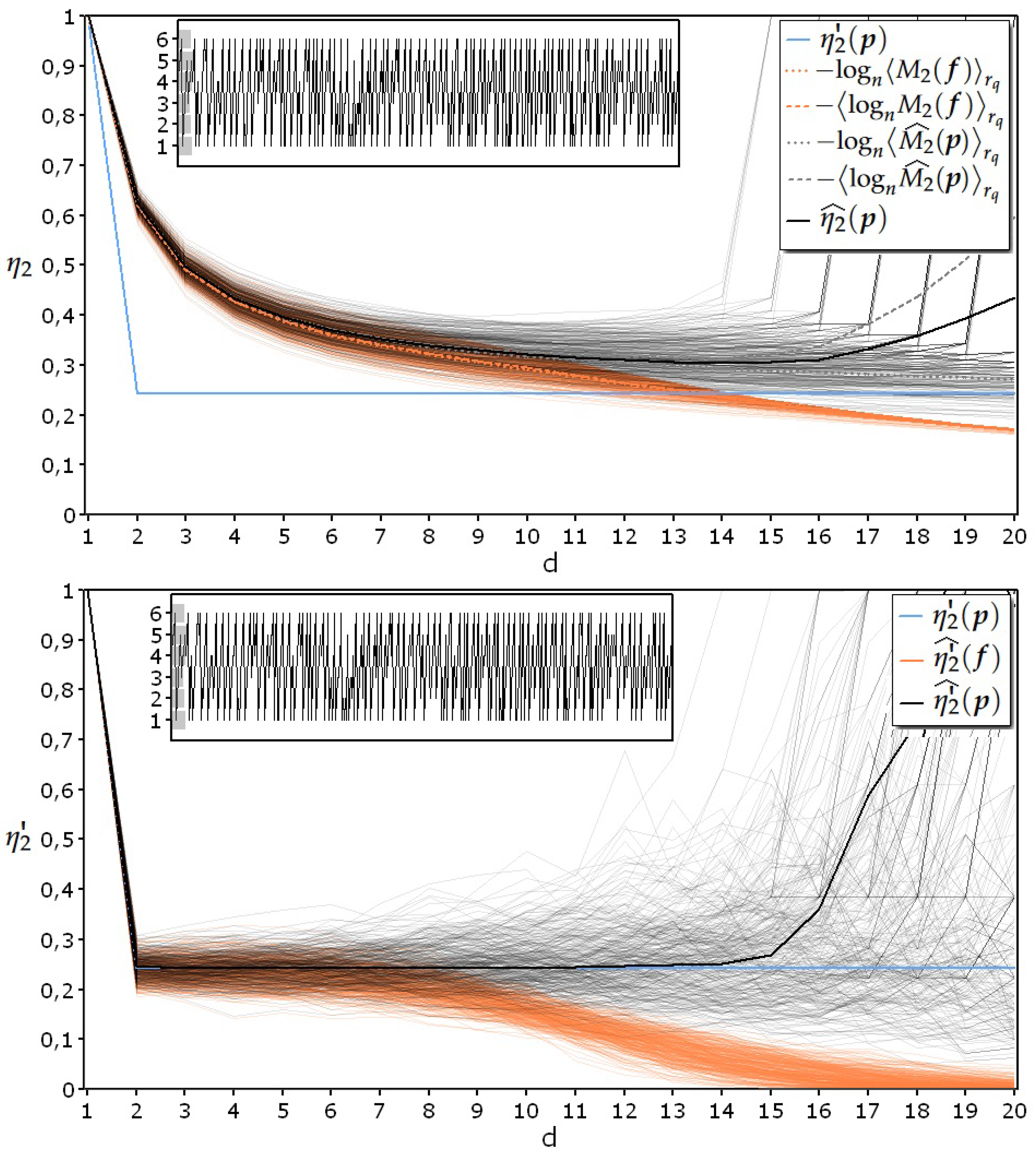
The upper diagram of Figure 2 shows that, in general, for processes whose samples have a dependence from the past, the trend of the estimated specific collision entropy, calculated using Formula (19), presents, at the beginning, a decrease, which depends on the progressive reduction of the topological ambiguity encountered during the detection of recurrences hidden in the data when the dimension of the sample space is increased. The curve subsequently rises due to the reduction of the density of the occurrences in the sample space. This corresponds to a reduction in the reliability of the information supplied by the relative frequencies; as a consequence, the uncertainty contained in the probability estimates grows, and the entropy increases accordingly. This ability to ramp up the curve when the estimate is no longer reliable is the second necessary prerequisite for an estimator. The observation of the diagrams of Figure 2 allow also to infer that

R F D

s cannot be used in place of

D P D

s because they intrinsically lack this capability. In fact, the use of the

R F D

s in the estimator gives poor results because their mean specific collision entropy seamlessly decreases even when the density of the data is actually no longer sufficient for producing any kind of estimation. In the middle of the curve, the minimum value of the specific collision entropy represents the best possible compromise between the request to observe in ever greater detail the regularities contained in the data and the limitations imposed by the shortness of the data. From Figure 2 it is also possible to establish a third necessary prerequisite that an entropy estimator must fulfill: in fact its output has always to be greater or equal than the corresponding theoretical value, because otherwise the estimator would erroneously signal the presence of an excessive amount of regularities in the process, thus violating the fundamental precaution principle required by all those situations in which statistical fluctuations are present. In a sentence: an estimator that expresses values of entropy higher than the correct theoretical ones is preferable to an estimator that expresses lower values.

Moreover, when the trend of the estimated specific collision entropy is compared with the trend of the estimated specific collision entropy rate, it becomes clear once again that this second index produces an impressively more rapid convergence towards the theoretical value (blue line) than the first one.

In the lower diagram of Figure 2 it is possible to see that the adherence of

\hat{η_{2}^{'}} (p)

η_{2}^{'} (p)

persists up to dimension 11; for this dimension the data density in the sample space results:

δ_{m i n} (M a r k o v, R = 300, N = 500) = \frac{L}{n} = \frac{N - d + 1}{q^{d}} = \frac{490}{6^{11}} = 1.35 \cdot 10^{- 6}

5.3. Experiments with Realizations Coming from Maximum Entropy Memoryless IID Processes

For the experiment whose results are reported in Figure 3, the input parameters are:

$D S P_{q}$ = process generated by tossing a loaded die with 50% of the outcomes equal to “1” ( $q = 6$ );
Upper diagram: $R = 2000$ and $N = 250$ ;
Lower diagram: $R = 500$ and $N = 1000$ .

From Formula (24) it results that

η_{2}^{'} (M a x E n t 50 %) = η_{2} (M a x E n t 50 %) = - \log_{6} 0.3 ≃ 0.672 .

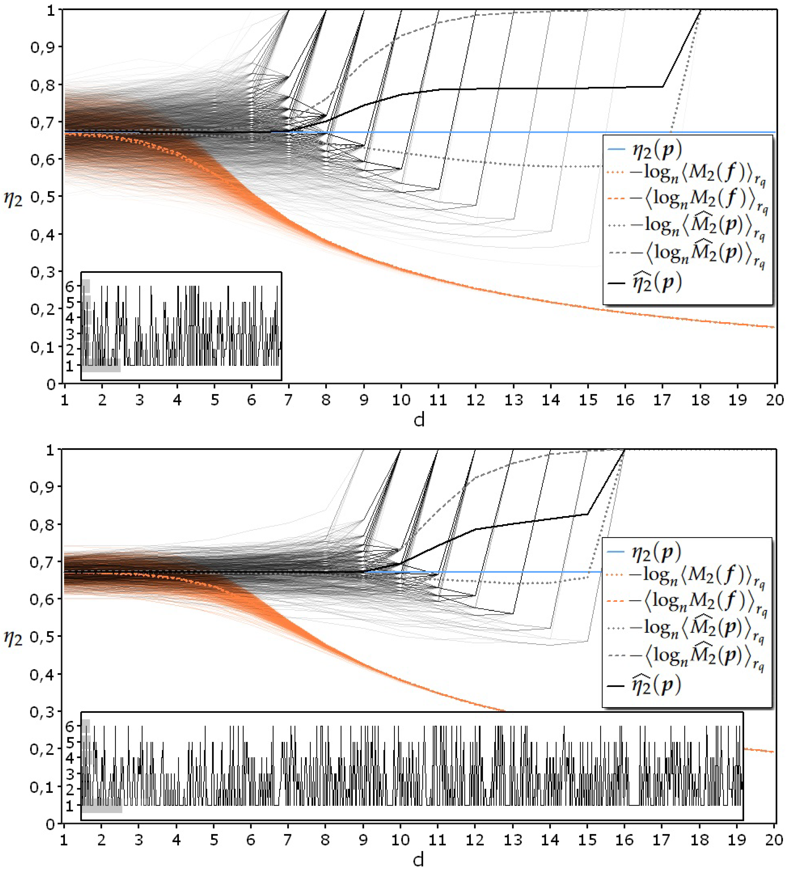
Both diagrams of Figure 3 show that:

the proposed estimator satisfies the aforementioned third prerequisite of never falling below the theoretical line, even in the heaviest test conditions, represented by the elaboration of data coming from a maximum entropy IID process;
when using $R F D$ s to estimate specific collision entropy, there is only a slight difference between the two possible ways of averaging the logarithm of the second raw moment (dotted and dashed lines in orange);
on the contrary, there is a remarkable difference between the two possible ways of averaging the estimates of the logarithm of the second raw moment (dotted and dashed lines in grey) as indicated in Formula (18);
when the data density in the sample space becomes insufficient for a reliable estimate of the entropy, its value rises toward the value corresponding to the uniform distribution.

In the upper diagram of Figure 3 it is possible to see that considering 250 samples per realization the adherence of

\hat{η_{2}} (p)

η_{2} (p)

persists up to dimension 6; for this dimension the data density in the sample space results:

δ_{m i n} (M a x E n t 50 %, R = 2000, N = 250) = \frac{L}{n} = \frac{N - d + 1}{q^{d}} = \frac{245}{6^{6}} = 5.25 \cdot 10^{- 3}

and the statistical fluctuations are considerable because of the shortness of the realizations. In the lower diagram of Figure 3 it is possible to see that considering 1000 samples per realization the adherence of

\hat{η_{2}} (p)

η_{2} (p)

persists up to dimension 9 (three dimensions more than the other situation); for this dimension the data density in the sample space results:

δ_{m i n} (M a x E n t 50 %, R = 500, N = 1000) = \frac{L}{n} = \frac{N - d + 1}{q^{d}} = \frac{992}{6^{9}} = 9.84 \cdot 10^{- 5}

and the statistical fluctuations are reduced because of the greater number of samples of each realization. From the comparison of the two diagrams, it can be seen that the increment in the availability of the data improves all the performance indicators of the estimator, and this fact proves its consistency even in the most severe test conditions. In general, to obtain an adequate horizontal trend of

\hat{η_{2}^{'}}

for at least two consecutive dimensions, it is necessary to rely on a sufficiently large number of samples per realization N or, alternatively, on a sufficiently high number of realizations R. The total number of aggregated samples (i.e., R x N) necessary for a good result of the estimation depends on the effective degree of irregularity of the signal. In fact, for completely regular processes with an alphabet composed of few symbols, even only

5 q

samples are sufficient for a correct estimate. In contrast, for almost random processes, at least

1, 000, 000

aggregated samples seem to be necessary.

Finally, concerning the hypothesis made at the beginning about the possibility of estimating the second raw moment of the

D P D

s coming from any kind of

D S P_{q}

using Formula (15), the evidences that emerged from the results of the experiments made for the validation of the estimator have not provided any counterexample that may exclude its validity. For this reason, the following statistics postulate is proposed:

Postulate

Given a sample space

Ω (q, d)

with cardinality

n = q^{d}

, and given a set of relative frequency distributions

{f {(Ω (q, d))}_{r_{q}}}_{D S P_{q}}

, each composed of L occurrences, resulting from the transformation of R short realizations

r_{q}

taken from the underlying discrete stochastic process

D S P_{q}

, to which an unknown discrete probability distribution

p (Ω (q, d))

is associated, then the unbiased and consistent estimator of the second raw moment of

p (Ω (q, d))

is inferred as

\forall D S P_{q} {\hat{M_{2} (p)}}_{D S P_{q}} = {〈m a x \{M_{2} (f) - \frac{1}{L}, \frac{1}{n}\}〉}_{r_{q}} .

6. Conclusions

Figure 2 and Figure 3 show that the proposed specific collision entropy rate estimator

\hat{η_{2}^{'}}

allows a very prolonged and consistent stay of its output, exactly at the values expected by the theory. This highly desirable and very uncommon feature, the simplicity of its formula and its complete usability with any discrete stationary process make this estimator a valid tool, suitable for measuring the degree of irregularity in experimental data from the perspective given by the collision entropy. Possible future research directions include:

the evaluation of the admissibility of this estimator by comparing it to other similar estimators and by using the same kind of processes for the tests;
the characterization of the variability of the values returned by the estimator $\hat{η_{2}^{'}}$ as the number of aggregated samples and the irregularity of the processes vary;
further studies on the methods of estimation in presence of the logarithm operator.

Funding

This research received no external funding.

Conflicts of Interest

The author declares no conflict of interest.

Abbreviations

The following abbreviations are used in this manuscript:

A	alphabet composed of q ordered symbols
$Ω (q, d)$	Sample space resulting from the Cartesian product d times of the alphabet A
$n = q^{d}$	cardinality of the sample space $Ω (q, d)$
$D S P_{q}$	Discrete-state stochastic process using an alphabet A
$D P D$	Generic discrete probability distribution
$p {(Ω (q, d))}_{D S P_{q}}$	$D P D$ obtained from a $D S P_{q}$ whose d-grams are inserted in $Ω (q, d)$
$r_{q}$	Realization of a $D S P_{q}$
$R F D$	Relative frequency distribution
$f {(Ω (q, d))}_{r_{q}}$	$R F D$ obtained from a realization $r_{q}$ of a $D S P_{q}$ whose d-grams are inserted in $Ω (q, d)$
$M_{2} (f)$	Second raw moment of an $R F D$
$M_{2} (p)$	Second raw moment of a $D P D$
$\hat{M_{2}} (p)$	Estimate of the second raw moment of a $D P D$
$H_{2} (f)$	Collision entropy of an $R F D$
$H_{2} (p)$	Collision entropy of a $D P D$
$\hat{H_{2}} (p)$	Estimated collision entropy of a $D P D$
$η_{2} (f)$	Specific collision entropy of an $R F D$
$η_{2} (p)$	Specific collision entropy of a $D P D$
$\hat{η_{2}} (p)$	Estimated specific collision entropy of a $D P D$
$η_{2}^{'} (f)$	Specific collision entropy rate of an $R F D$
$η_{2}^{'} (p)$	Specific collision entropy rate of a $D P D$
$\hat{η_{2}^{'}} (p)$	Estimated specific collision entropy rate of a $D P D$

References

Rényi, A. On measures of entropy and information. In Proceedings of the Proceedings of the Fourth Berkeley Symposium on Mathematical Statistics and Probability, Volume 1: Contributions to the Theory of Statistics, Berkeley, CA, USA, 1961; pp. 547–561.
Grassberger, P. Finite sample corrections to entropy and dimension estimates. Physics Letters A 1988, 128, 369–373. [Google Scholar] [CrossRef]
Cachin, C. Smooth Entropy and Rényi Entropy. In Proceedings of the Advances in Cryptology — EUROCRYPT ’97; Fumy, W., Ed. Springer-Verlag, 5 1997, Vol. 1233, Lecture Notes in Computer Science, pp. 193–208.
Schmitt, A.; Herzel, H. Estimating the Entropy of DNA Sequences. Journal of theoretical biology 1997, 188, 369–77. [Google Scholar] [CrossRef]
Holste, D.; Große, I.; Herzel, H. Bayes’ estimators of generalized entropies. Journal of Physics A: Mathematical and General 1998, 31, 2551–2566. [Google Scholar] [CrossRef]
Strong, S.P.; Koberle, R.; de Ruyter van Steveninck, R.R.; Bialek, W. Entropy and Information in Neural Spike Trains. Phys. Rev. Lett. 1998, 80, 197–200. [Google Scholar] [CrossRef]
de Wit, T.D. When do finite sample effects significantly affect entropy estimates? The European Physical Journal B - Condensed Matter and Complex Systems 1999, 11, 513–516. [Google Scholar] [CrossRef]
Antos, A.; Kontoyiannis, I. Convergence properties of functional estimates for discrete distributions. Random Structures & Algorithms 2001, 19, 163–193. [Google Scholar] [CrossRef]
Nemenman, I.; Shafee, F.; Bialek, W. Entropy and inference, revisited. In T. G. Dietterich, S. Becker, and Z. Ghahramani, editors, Advances in Neural Information Processing Systems 2002, 14, 471–478. [Google Scholar]
Paninski, L. Estimation of entropy and mutual information. Neural Computation 2003, 15, 1191–1253. [Google Scholar] [CrossRef]
Chao, A.; Shen, T.J. Non parametric estimation of Shannon’s index of diversity when there are unseen species. Environ. Ecol. Stat. 2003, 10, 429–443. [Google Scholar] [CrossRef]
Schürmann, T. Bias analysis in entropy estimation. Journal of Physics A: Mathematical and General 2004, 37, L295. [Google Scholar] [CrossRef]
Paninski, L. Estimating entropy on m bins given fewer than m samples. IEEE Transactions on Information Theory 2004, 50, 2200–2203. [Google Scholar] [CrossRef]
Bonachela, J.; Hinrichsen, H.; Muñoz, M. Entropy estimates of small data sets. Journal of Physics A: Mathematical and Theoretical 2008, 41, 9. [Google Scholar] [CrossRef]
Grassberger, P. Entropy Estimates from Insufficient Samplings, 2008, [arXiv:physics.data-an/physics/0307138].
Hausser, J.; Strimmer, K. Entropy inference and the James-Stein estimator, with application to nonlinear gene association networks. J. Mach. Learn. Res. 2009, 10, 1469–1484. [Google Scholar]
Lesne, A.; Blanc, J.; Pezard, L. Entropy estimation of very short symbolic sequences. Physical Review E 2009, 79, 046208. [Google Scholar] [CrossRef]
Xu, D.; Erdogmuns, D. Renyi’s Entropy, Divergence and Their Nonparametric Estimators. In Information Theoretic Learning: Renyi’s Entropy and Kernel Perspectives; Springer New York: New York, NY, 2010; pp. 47–102. [Google Scholar] [CrossRef]
Vinck, M.; Battaglia, F.; Balakirsky, V.; Vinck, A.; Pennartz, C. Estimation of the entropy based on its polynomial representation. Phys. Rev. E 2012, 85, 051139. [Google Scholar] [CrossRef] [PubMed]
Valiant, G.; Valiant, P. Estimating the Unseen: Improved Estimators for Entropy and Other Properties. J. ACM 2017, 64. [Google Scholar] [CrossRef]
Zhang, Z.; Grabchak, M. Bias Adjustment for a Nonparametric Entropy Estimator. Entropy 2013, 15, 1999–2011. [Google Scholar] [CrossRef]
Acharya, J.; Orlitsky, A.; Suresh, A.; Tyagi, H. The complexity of estimating Rényi entropy. In Proceedings of the Proceedings of the twenty-sixth annual ACM-SIAM symposium on Discrete algorithms. SIAM, 2014, pp. 1855–1869.
Archer, E.; Park, I.; Pillow, J. Bayesian entropy estimation for countable discrete distributions. The Journal of Machine Learning Research 2014, 15, 2833–2868. [Google Scholar]
Li, L.; Titov, I.; Sporleder, C. Improved estimation of entropy for evaluation of word sense induction. Computational Linguistics 2014, 40, 671–685. [Google Scholar] [CrossRef]
Acharya, J.; Orlitsky, A.; Suresh, A.; Tyagi, H. , The complexity of estimating Rényi entropy. In Proceedings of the 2015 Annual ACM-SIAM Symposium on Discrete Algorithms (SODA); pp. 1855–1869.
Zhang, Z.; Grabchak, M. Entropic representation and estimation of diversity indices. Journal of Nonparametric Statistics 2016, 28, 563–575. [Google Scholar] [CrossRef]
Acharya, J.; Orlitsky, A.; Suresh, A.; Tyagi, H. Estimating Rényi entropy of discrete distributions. IEEE Transactions on Information Theory 2017, 63, 38–56. [Google Scholar] [CrossRef]
de Oliveira, H.; Ospina, R. A Note on the Shannon Entropy of Short Sequences 2018. [CrossRef]
Berrett, T.; Samworth, R.; Yuan, M. Efficient multivariate entropy estimation via k-nearest neighbour distances. The Annals of Statistics 2019, 47, 288–318. [Google Scholar] [CrossRef]
Verdú, S. Empirical estimation of information measures: a literature guide. Entropy 2019, 21, 720. [Google Scholar] [CrossRef]
Goldfeld, Z.; Greenewald, K.; Niles-Weed, J.; Polyanskiy, Y. Convergence of smoothed empirical measures with applications to entropy estimation. IEEE Transactions on Information Theory 2020, 66, 4368–4391. [Google Scholar] [CrossRef]
Contreras Rodríguez, L.; Madarro-Capó, E.; Legón-Pérez, C.; Rojas, O.; Sosa-Gómez, G. Selecting an effective entropy estimator for short sequences of bits and bytes with maximum entropy. Entropy 2021, 23. [Google Scholar] [CrossRef]
Kim, Y.; Guyot, C.; Kim, Y. On the efficient estimation of Min-entropy. IEEE Transactions on Information Forensics and Security 2021, 16, 3013–3025. [Google Scholar] [CrossRef]
Grassberger, P. On Generalized Schürmann Entropy Estimators. Entropy 2022, 24. [Google Scholar] [CrossRef]
Pincus, S. Approximate entropy as a measure of system complexity. Proc Nati.Acad.Sci.USA 1991, 88, 2297–2301. [Google Scholar] [CrossRef] [PubMed]
Richman, J.S.; Moorman, J.R. Physiological time-series analysis using approximate entropy and sample entropy. American Journal of Physiology-Heart and Circulatory Physiology 2000, 278, H2039–H2049. [Google Scholar] [CrossRef] [PubMed]
Manis, G.; Aktaruzzaman, M.; Sassi, R. Bubble entropy: An entropy almost free of parameters. IEEE Transactions on Biomedical Engineering 2017, 64, 2711–2718. [Google Scholar] [CrossRef]
Shannon, C. The bandwagon (Edtl.). IRE Transactions on Information Theory 1956, 2, 3–3. [Google Scholar] [CrossRef]
Ribeiro, M.; Henriques, T.; Castro, L.; Souto, A.; Antunes, L.; Costa-Santos, C.; Teixeira, A. The entropy universe. Entropy 2021, 23. [Google Scholar] [CrossRef] [PubMed]
Skorski, M. Improved estimation of collision entropy in high and low-entropy regimes and applications to anomaly detection. Cryptology ePrint Archive, Paper 2016/1035, 2016.
Skorski, M. Towards More Efficient Rényi Entropy Estimation. Entropy 2023, 25, 185. [Google Scholar] [CrossRef] [PubMed]
Shannon, C. A mathematical theory of communication. The Bell System Technical Journal 1948, 27, 379–423. [Google Scholar] [CrossRef]
Kamath, S.; Verdú, S. Estimation of entropy rate and Rényi entropy rate for Markov chains. In Proceedings of the 2016 IEEE International Symposium on Information Theory (ISIT); 2016; pp. 685–689. [Google Scholar] [CrossRef]
Golshani, L.; Pasha, E.; Yari, G. Some properties of Rényi entropy and Rényi entropy rate. Information Sciences 2009, 179, 2426–2433. [Google Scholar] [CrossRef]
Golshani, L.; Pasha, E. Rényi entropy rate for Gaussian processes. Information Sciences 2010, 180, 1486–1491. [Google Scholar] [CrossRef]
Teixeira, A.; Matos, A.; Antunes, L. Conditional Rényi Entropies. IEEE Transactions on Information Theory 2012, 58, 4273–4277. [Google Scholar] [CrossRef]
Fehr, S.; Berens, S. On the Conditional Rényi Entropy. IEEE Transactions on Information Theory 2014, 60, 6801–6810. [Google Scholar] [CrossRef]
Packard, N.H.; Crutchfield, J.P.; Farmer, J.D.; Shaw, R.S. Geometry from a Time Series. Phys. Rev. Lett. 1980, 45, 712–716. [Google Scholar] [CrossRef]
Takens, F. Detecting strange attractors in turbulence. In Proceedings of the Dynamical Systems and Turbulence, Warwick 1980: proceedings of a symposium held at the University of Warwick 1979/80. Springer, 1981-2006, pp. 366–381.

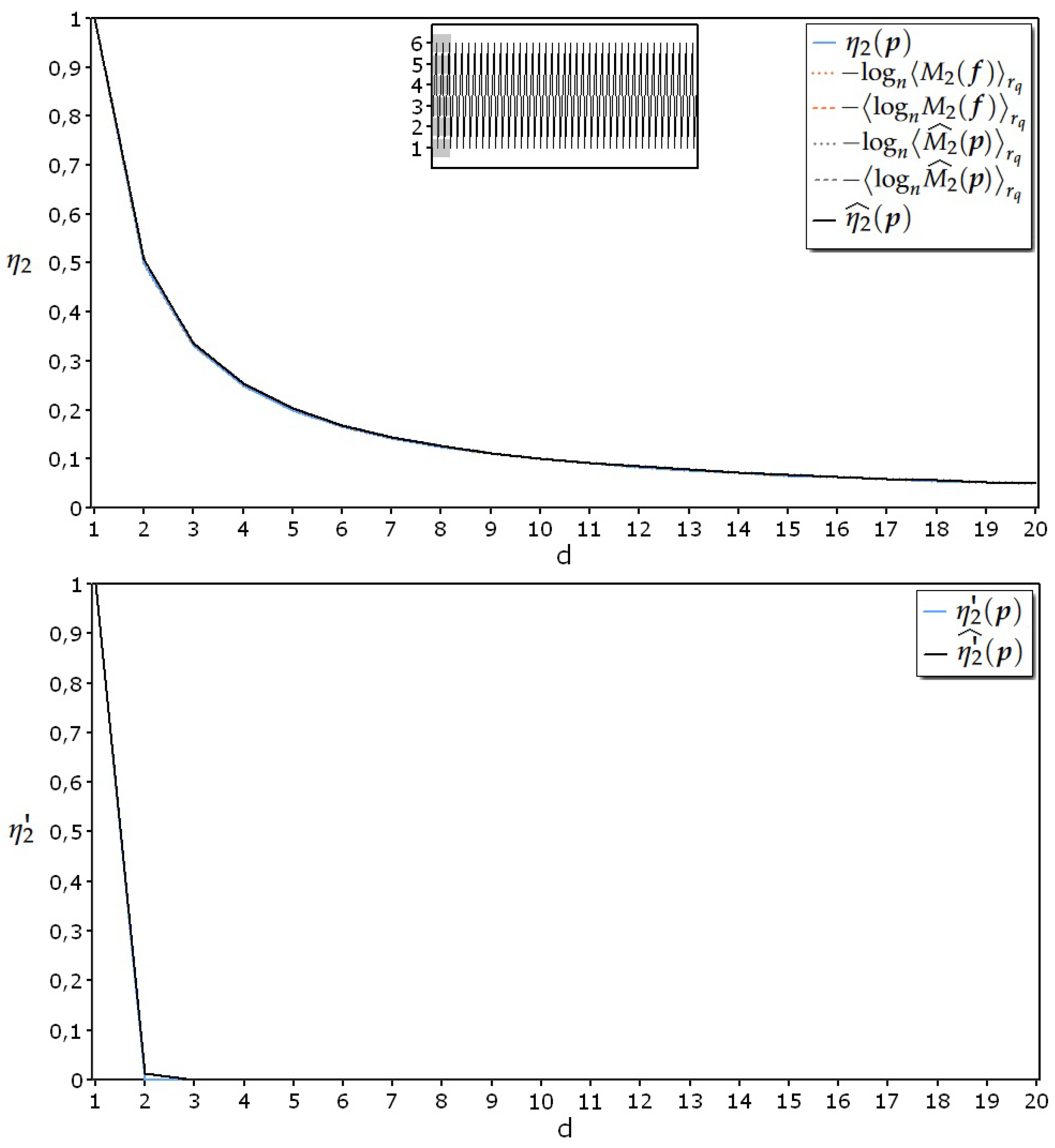
Figure 1. Trend of

η_{2}

(upper diagram) and trend of

η_{2}^{'}

(lower diagram) for a realization composed of 250 samples taken from a regular process.

Figure 1. Trend of

η_{2}

(upper diagram) and trend of

η_{2}^{'}

(lower diagram) for a realization composed of 250 samples taken from a regular process.

Figure 2. Trends of

η_{2}

(upper diagram) and

η_{2}^{'}

(lower diagram) for 300 realizations, each composed of 500 samples taken from the Markovian process described by the previous transition matrix

p_{66}

and stationary distribution

μ_{6}^{*}

Figure 2. Trends of

η_{2}

(upper diagram) and

η_{2}^{'}

(lower diagram) for 300 realizations, each composed of 500 samples taken from the Markovian process described by the previous transition matrix

p_{66}

and stationary distribution

μ_{6}^{*}

Figure 3. Trends of

η_{2}

for the realizations of a process generated by tossing a loaded die with 50% of the outcomes equal to “1”. Upper diagram: 2000 realizations, each 250 samples long; lower diagram: 500 realizations, each 1000 samples long.

Figure 3. Trends of

η_{2}

Disclaimer/Publisher’s Note: The statements, opinions and data contained in all publications are solely those of the individual author(s) and contributor(s) and not of MDPI and/or the editor(s). MDPI and/or the editor(s) disclaim responsibility for any injury to people or property resulting from any ideas, methods, instructions or products referred to in the content.

© 2023 by the authors. Licensee MDPI, Basel, Switzerland. This article is an open access article distributed under the terms and conditions of the Creative Commons Attribution (CC BY) license (http://creativecommons.org/licenses/by/4.0/).

Copyright: This open access article is published under a Creative Commons CC BY 4.0 license, which permit the free download, distribution, and reuse, provided that the author and preprint are cited in any reuse.

MDPI Initiatives

Important Links

Choose an area of interest and we will send you notifications of new preprints at your preferred frequency.

Disclaimer

Collision Entropy Estimation in a One-Line Formula

Abstract

1. Introduction

2. Theoretical Methods

2.1. Transforming a Discrete-State Stochastic Process into a DPD

2.2. Integer-Order Rényi α -Entropies as Synthetic Indices for the Characterization of D P D s

2.3. Rényi Entropy Rates

2.4. Specific Rényi Entropy Rate

2.5. Relationship between Specific Rényi Entropy Rate and Specific Rényi Entropy

3. Empirical Methods

3.1. Transforming a Realization into a Distribution of Relative Frequencies

3.2. Estimating the Second Raw Moment of a D P D

3.3. Estimating the Specific Collision Entropy of a D S P q

3.4. Estimating the Specific Collision Entropy Rate of a DSPq

3.5. Method of Validation of Entropy Estimators

4. Materials: Choice of Convenient D S P q s Suitable for the Experiments

5. Results and Discussion

5.1. Experiments with Realizations Coming from Completely Regular Processes

5.2. Experiments with Realizations Coming from Processes Presenting Some Sort of Regularity

5.3. Experiments with Realizations Coming from Maximum Entropy Memoryless IID Processes

6. Conclusions

Funding

Conflicts of Interest

Abbreviations

References

MDPI Initiatives

Important Links

Subscribe

2.2. Integer-Order Rényi $α$ -Entropies as Synthetic Indices for the Characterization of $D P D$ s

3.2. Estimating the Second Raw Moment of a $D P D$

3.3. Estimating the Specific Collision Entropy of a $D S P_{q}$

4. Materials: Choice of Convenient $D S P_{q}$ s Suitable for the Experiments