Preprint
Article

Investigation of Auxetic Structural Deformation Behavior of PBAT Polymers Using Process and Finite Element Simulation

Altmetrics

Downloads

123

Views

34

Comments

0

A peer-reviewed article of this preprint also exists.

Submitted:

21 May 2023

Posted:

22 May 2023

You are already at the latest version

Alerts
Abstract
The current work investigates the auxetic tensile deformation behavior of the inversehoneycomb structure with 5 × 5 cells made of biodegradable poly(butylene adipate-coterephthalate) (PBAT). Fused deposition modeling, an additive manufacturing method, produced such specimens. Residual stress (RS) and warpage, more or less, always exist in such specimens due to layer-by-layer fabrication, i.e., repeated heating and cooling. The RS influences the auxetic deformation behavior, but its measurement is challenging due to the very fine structure. Instead, the finite-element(FE)-based process simulation realized by an ABAQUS plug-in numerically predicts the RS and warpage. The predicted warpage shows a negligible slight deviation compared to the design topology. This process simulation also delivers the temperature evolution of a small volume material, revealing the local cyclic heating and cooling. The achieved RS serves as the initial condition for the FE model used to investigate the auxetic tensile behavior. With the outcomes from FE calculation without considering RS at hand, the effect of the RS on the deformation behavior is discussed for the global force-displacement curve, the structural Poisson’s ratio evolution, the deformed structural status, the stress distribution, and evolution, where the first three and the warpage are also compared with experimental results. Furthermore, the FE simulation can easily provide the global stress-strain flow curve with the total stress calculated from the elemental ones.
Keywords: 
Subject: Engineering  -   Other

1. Introduction

A promising class of materials for structural components is metal materials with auxetic behavior. Auxetic structures own a negative Poisson’s ratio [1], which means such structures behave counterintuitively. They are generally cellular and also called auxetic 5 materials. Detailed descriptions of Poisson’s ratios can be referred to [1, 2, 3, 4, 5, 6, 7, 8], which present both general definition of the Poisson’s ratio and specific deduction of auxetic cells. Most existing auxetic structures are synthetic ones [9], so-called mechanical metamaterials. A few natural ones are found, e.g., reported in [10, 11, 12]. A review of auxetic structures is given in Kelkar et al. [13] and Negrea [14]. In producing auxetic 10 structures, additive manufacturing (AM) has provided an efficient production process from design to prototype and final applicable components. This technique also allows the quick production of complex geometries. 3D printing belongs to AM. Some review articles about AM can be found in [15, 16, 17]. The layer-by-layer production process causes reheating of underlying materials near the place of extrusions. Still, reheated materials 15 also undergo repeated cooling. These heating-cooling cycles, besides the type of contract between the printed part and the build part, result in residual stresses (RSes) in the structure. In order to obtain knowledge of the RS in the structure after printing, numerical prediction can be used, e.g. finite element (FE) simulation.
This work is a continuation of Schneider et al. [18]. In the current work, the biodegra-20 dable poly(butylene adipate-co-terephthalate) (PBAT) is preferred as sample material, which is commercially available. The aim is to investigate the tensile deformation characteristics of auxetic structures. Experiments and FE simulations, including the FE-based process simulation, are performed. The inverse honeycomb shape, a type of re-entrant structure, is selected. The RS, more or less, exists in the specimen. In this work, RS is 25 predicted by a FE-based process simulation, which is realized through an ABAQUS plugin “AM Modeler” [19, 20]. Such simulation enables the consideration of the RS in the FE simulation for subsequent tensile tests. It refers to Hufert et al. [21] and Schneider et al. [18] for the detailed description of the experiments. The comparison is performed between experimental and numerical results, including with and without considering RS.

2. Material and Experiment

Commercial PBAT Ecoflex F Blend C1200, a fully biodegradable plastic, was purchased from BASF, Ludwigshafen, Germany. A schematic illustration of the PBAT’s chemical structure can be referred to [22, 23]. It refers to Hufert et al. [21] and Schneider et al. [18] for some detailed description of the material.
35 The tensile flow behavior of a standard specimen is used to calibrate the FE-simulated stress-strain behavior in searching for a suitable material model (theory) to predict PBAT deformation behavior. The tensile specimen is printed according to DIN EN ISO 527-1 standard. Generally, the same test is repeated no less than five times. The experimental results [18, 21], Young’s modulus, yield stress Rp0.2, ultimate tensile strength and strain, 40 and stress-strain flow behavior, are comparable with those found in literature [24, 25]. The mean value of all measured data is used for comparison with numerical predictions in this work. Furthermore, both measurement [21] and FE simulation [18] found that an auxetic structure with 5 × 5 cells is the optimum one among 3 × 3, 5 × 5, and 7 × 7 to represent the auxetic behavior well. Still, this selection of 5 × 5 cells is material independent. It 45 means the experimental and numerical studies emphasized structures with 5 × 5 cells. The dimensions of a unit cell and this 5 × 5 structure are presented in [18, 21]. The results of auxetic structural deformation behavior, such as the force-displacement curve, deformed status according to loading, calculation methods of Poisson’s ratio, and the evolution of Poisson’s ratio are referred to [18]. In case of no other specification, all the 50 tests are performed at the IKT Institute, University of Stuttgart, Germany.
The in-situ micro-computed tomography (µCT) is performed in RIF e. V. Dortmund, Germany. The tests have been carried out with the v |tome| x L 240 (GE Sensing & Inspection Technologies GmbH, Wunstorf, Germany). For PBAT, the test parameter is 120 keV and 80 µA with a voxel size of 25 µm. Limited by the vertical space of the testing 55 rig and PBAT’s extra high tensile deformation ability, the auxetic specimen with 3 × 3 cells is used. Four scans were performed at loadings of 0, 5, 10, and 15 mm. Hufert et al. [21] presented more detailed descriptions of the test and measured results.

3. Process and FE Simulation

In order to numerically predict the auxetic structural deformation behavior, FE cal60 culations covering cases of the (printing) process and mechanical loading simulation are performed. The former delivers the warpage and RSes for the latter. Practically, the RS is mapped to the mechanical loading simulation, and the warpage is omitted since it is negligibly small. The RS is estimated to be low, around one MPa. Here, a numerical calculation of the RS is done using the process simulation, which is realized by an ABAQUS 65 plug-in called ”AM Modeller” [20]. It employs the toolpath-meshing intersection module and a few subroutines to assist the calculations [19] and provides an additional interface to define new parameters to set up the simulation. The user interface is subdivided into three parts: data setup, model setup, and simulation setup. The event series and table collection are defined in the data setup part and list time, location, and power values, 70 representing the printing path. The event series originated from G-code, a programming language widely used by various manufacturing machines [26]. The machine controller reads the G-code to regulate the motors for their moving direction and velocity [26]. The following subsection 3.1 describes the process simulation steps in more detail and the model used in this work. The model set-sup for the mechanical FE simulation is referred 75 to Schneider et al. [18]. Here, only a brief introduction is given in subsection 3.2.

3.1. Simulation of additive manufacturing using FE method

3.1.1. Approach of additive manufacturing process simulation

The advantages of AM simulations can be predicting RSes in part, minimizing differences between the part design and the manufactured part, and numerical evaluating part 80 performance under real load conditions. ABAQUS offers the toolpath-mesh intersection function for AM simulations. This function enables the detection of geometric intersections between a toolpath and an FE meshing of a part to be manufactured. ABAQUS has two methods for simulating AM processes: a thermomechanical and an eigenstrain-based simulation. The latter has been successfully used to evaluate RSes from welding proces- 85 ses. The results obtained by this method are usually more accurate compared to those obtained by thermomechanical simulation. The main drawback of the latter is that more effort is required to calibrate the eigenstrain values either by experiments or by running other simulations.
The thermomechanical simulation requires a separation of the simulation into two 90 parts: a heat transfer analysis is performed using a thermal model first, and then a stress analysis is conducted using a mechanical model to calculate the deformations in the component and the stress distribution. The heat transfer analysis delivers the evolution of the temperature distribution based on a moving heat source and thermal boundary conditions, such as convection, conduction, or radiation. This temperature distribution, presented as 95 the temperature at each node in every time increment, is then transferred to the stress analysis as a predefined field. Finally, the deformations and stresses can be calculated with the mechanical constraints. With this method, it is possible to include machine information and process parameters, such as laser power, layer thickness, toolpath, support structures, and a substrate where the part and the support are built, in order to evaluate 100 their influences on thermal behavior, part distortions, and residual stresses.
Sequential thermomechanical simulation of the additive manufacturing process. The AM simulation has to include the typical characteristics of the 3D printing process: a progressive material deposition, a progressive heating of the deposited material, and a progressive cooling of the printed part. The progressive material deposition is mo105 deled using the progressive element activation function provided by ABAQUS/Standard. Elements with this characteristic can be either partially or completely filled with material or simply remain empty, i.e., inactive. The material deposition is defined through a so-called “event series”, which defines the time and space coordinates. Still, event series also define the objective of controlling the amount of material added to an element in a 110 given time increment.
Thermal Analysis. The conducted three-dimensional heat transfer analysis is governed by the heat transfer energy balance, which is written as:
Preprints 74253 i001
where ρ, Cp, T, t, Q, and r are the material density, the specific heat capacity, the temperature, the time, the heat source, and the relative reference coordinate, respectively. q is the heat flux vector, calculated as:
q = −k∇T,
where k is the thermal conductivity of the material. The thermal condition on the boundaries is described by the mechanism’s radiation, conduction, or convection. The first mechanism depends on the surface quality and the color, affecting emissivity. Radiation and convection are due to heat loss into the environment via the component’s surface. Conduction is observed if the component is in contact with another component, which could be a substrate or fixation to position the component. In comparison, convection depends on the surrounding medium and the flow behavior of this medium. The heat flux on a surface due to convection is governed by:
q = −h(TT0)
where h is the coefficient of convection and T0 is the ambient temperature. Due to missing data to assign a certain amount of heat loss on a surface by radiation, the effect of radiation is taken into account as part of convection.
In the process simulation, a moving heat source represents the laser or heat source, 115 which assigns a calculated heat flux to a defined volume. Such a heat flux distribution within a defined volume can be calculated by using different formulations. In the past, the heat source models introduced the heat at the surface of the component, such as the circular disc model proposed by Pavelic et al., which describes a Gaussian surface flux distribution on the surface of a component [27]. Further investigations lead to the 120 development of a hemi-spherical power density distribution or ellipsoidal power density distribution to introduce the heat within a volume.
In ABAQUS, three different ways can define the shape of the moving heat source. The first one is in the form of a moving concentrated heat flow. This is recommended when the size of the finite elements is significantly larger than the size of the laser spot. When the laser spot size is comparable to the element size, it is recommended to specify the moving heat source with a so-called Goldak distribution or a uniform distribution. The first is a double ellipsoidal power density distribution often used in welding simulations. The second one distributes the laser power uniformly over a box-shaped volume. Then, the volumetric heat power Pvol is calculated as follows:
Preprints 74253 i002
where η is the absorption coefficient, Plaser the laser power, v the scan speed of the AM process, w the width of the box-shaped volume, and h the height of the box-shaped volume. The heat source is then defined by the basic geometry. The absorption coefficient 125 η depends on the optical properties of the material, the laser wavelength, and the surface temperature [28]. For the FDM process, the nozzle represents the laser, which extrudes the molten filament. In this case, the absorption coefficient is assumed to be one.
Mechanical analysis. The stress analysis requires the set-up of a mechanical model first. Then, the stresses and the deformations are determined by performing a three-dimensional quasi-static incremental analysis. Finally, the build plate needs to be constrained to represent the experimental conditions to avoid rigid body movement. The mechanical analysis is performed under the consideration of a quasi-static equilibrium state. The contact between the build plate and the printed part is assumed to be ideal. The mechanical load or thermal stress σth results from the applied temperature evolution and the different thermal expansion coefficients of the build plate material and the printed material, which is given by:
σth = Eα(T − T0),
where E is the Young’s modulus and α the thermal expansion coefficient. Plastic deformation at elevated temperatures, accompanied by the reduced yield strength compared 130 to room temperature, results in RSes contained in a solid material despite the absence of external forces. The RSes can be either tensile or compressive at a given place. Generally, a component contains a combination of both stresses because the sum of all RSes over the whole component needs to be zero.

3.1.2. Current process simulation

135 Components manufactured with the fused filament fabrication (FFF) process have warpage and RSes due to the layer-by-layer building and thermal differences in the volume [29]. Additionally, materials with a high coefficient of thermal expansion are prone to experience more deformation in the AM process [30]. Hence, the material model in process simulation needs various properties to be defined. The properties defined for this study are 140 density, elasticity, plasticity, specific heat, thermal expansion, and thermal conductivity. It refers to [19, 20, 31] for a more detailed description of the process simulation.
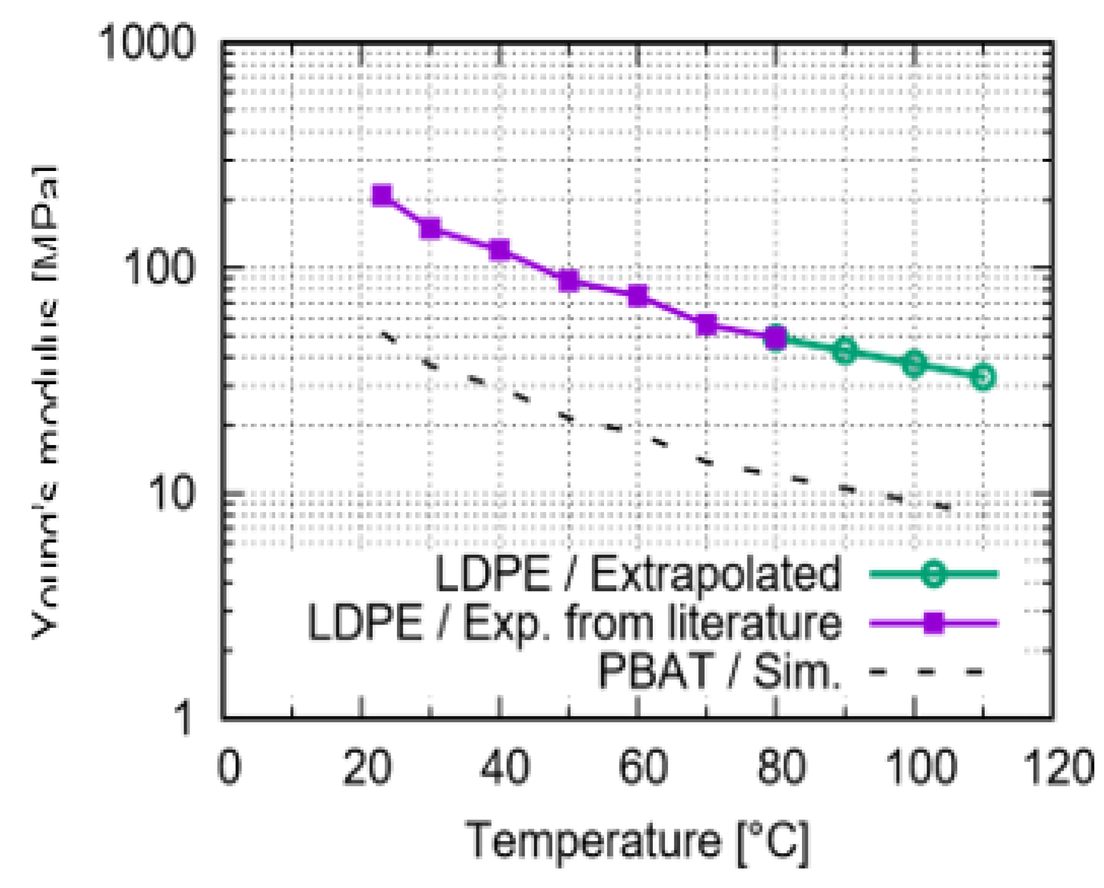
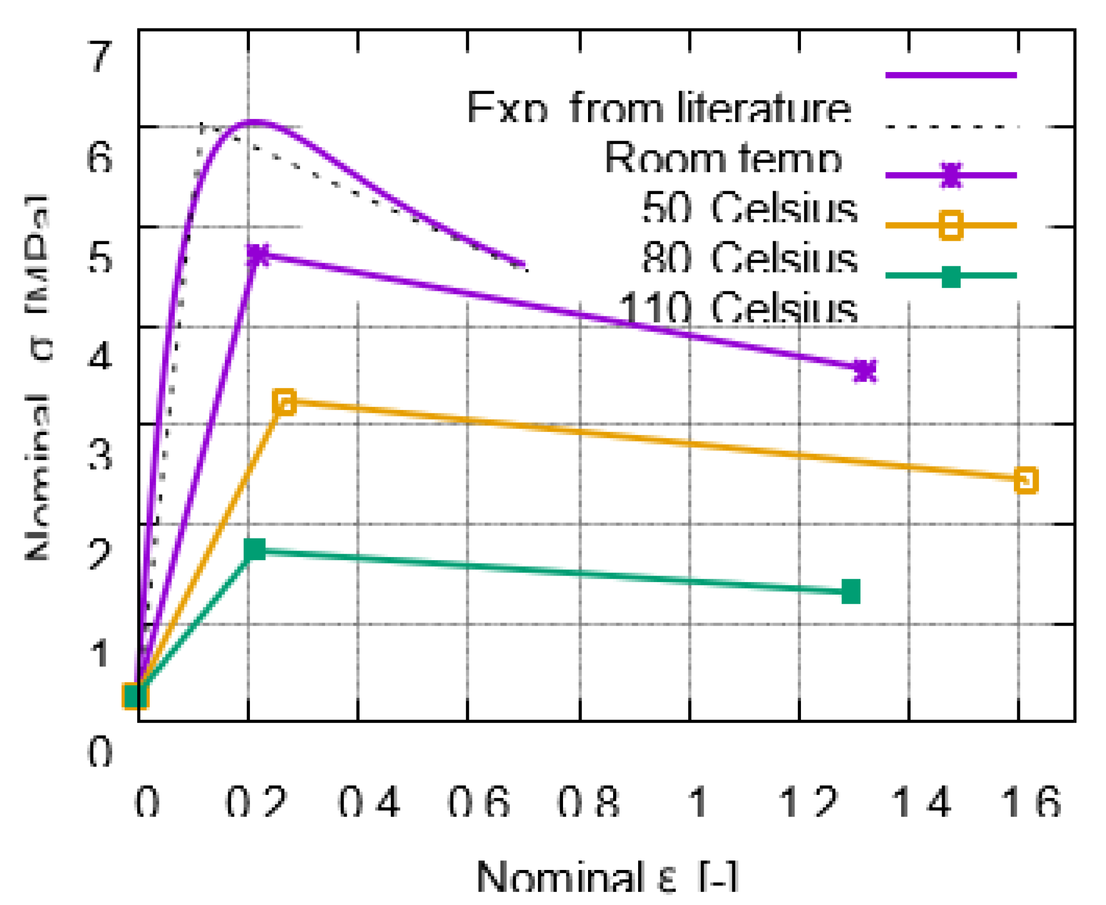
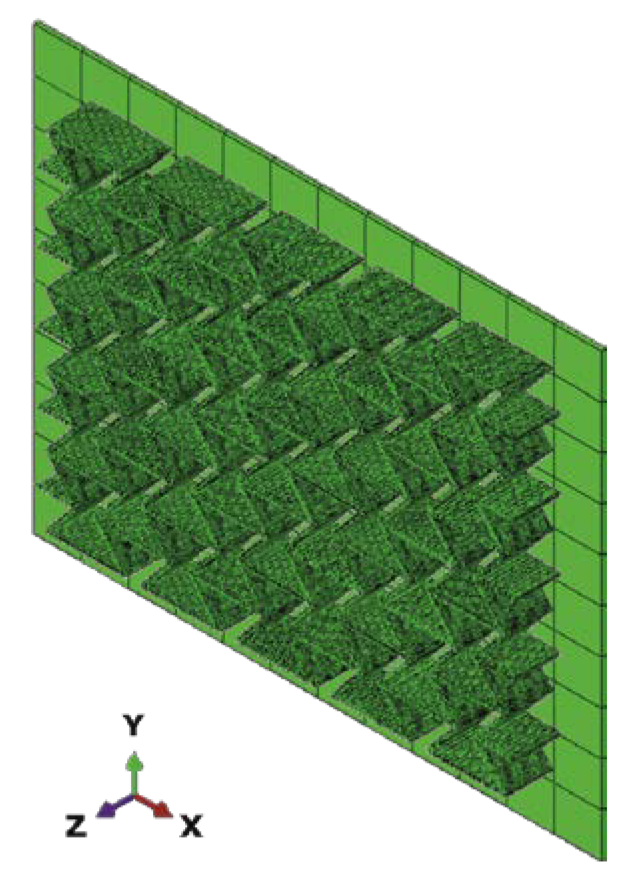
The melting temperature of PBAT is 110-120 C [25, 32]. Due to the available data for PBAT being limited from the current investigation and the literature, it is challenging to find its data at elevated temperatures. Thus, some of the required input data were 145 interpolated with the help of low-density polyethylene (LDPE) data in higher temperature regimes since PBAT and LDPE behave similarly under loading. LDPE is also a semi-crystalline polymer with a melting point of approximately 110 C [33, 34] and glass transition temperature of -32.2 C [33], which are comparable to the PBAT data. The Poisson’s ratio is assumed to be 0.41 for the entire temperature range. Fig. 1 presents 150 the temperature-dependent Young’s modulus of LDPE [35] and the estimated values of PBAT. These data are used in the current work. Fig. 2 denotes the estimated nominal stress-strain behavior at different temperatures, where the linear behavior fulfills the requirements of the ABAQUS plug-in mentioned above. The endpoint of the increasing part of each curve in Fig. 2 corresponds to the yield stresses at the given temperature. 155 Concerning the FE-based process simulation, Fig. 3 illustrates the meshed plate and the auxetic structure. The plate has a constant temperature of 60 C during the printing. The meshing of the auxetic structure is identical to the one used in the mechanical loading.
Figure 1. Temperature dependent LDPE.
Preprints 74253 g001
Figure 2. Estimated temperature-dependent ABAQUS plug-in [19]. Young’s modulus values for elasticity model [35] and the estimated values for PBAT [35]. norminal stress-strain behavior for PBAT [35], where the linear behavior is the request of the.
Preprints 74253 g002
Figure 3. Meshing used in the process simulation and the plate with 60 C, where the meshing of the auxetic structure is identical in the FE and in the process simulation.
Preprints 74253 g003

3.2. FE simulation with mechanical loading
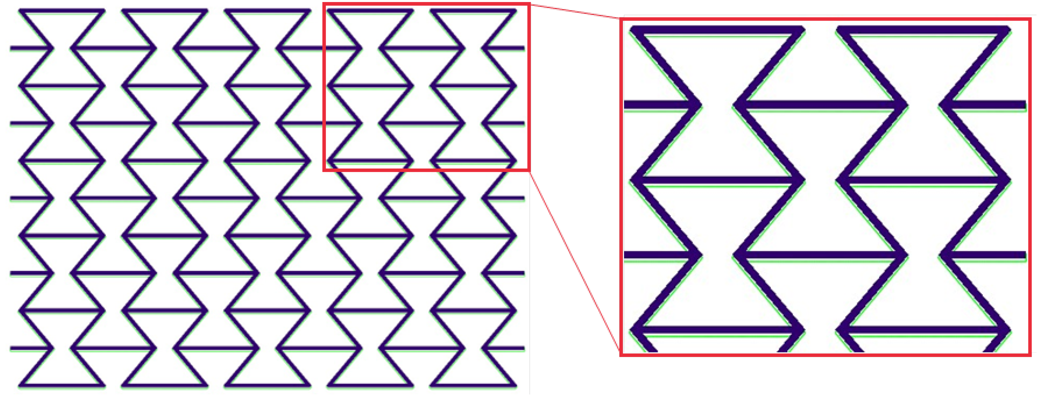
Using ABAQUS [19, 36] inherent functions (theory/material models) to predict the 160 polymer deformation behaviors is preferred. Schneider et al. [18] found that the “Ogden” model with N=4 is suitable for predicting the PBAT deformation behavior. There is a total of 738,760 octagonal and hexagonal elements with types of C3D8H and C3D6H. Detailed descriptions of the selection and a brief review of FE simulation applied for polymers can be referred to Schneider et al. [18]. The current work follows Schneider 165 et al. [18, 37], i.e., “Ogden N=4” model used. As mentioned, the predicted warpage caused by the printing process is negligible small, and to be simple, the current work used the initial CAD-design geometry, which is identical to the meshed structure applied for process simulation (Fig. 3). Fig. 4 illustrates the overlay view of the initial CAD-design geometry and the predicted deformed state after cooling, where the green contour presents 170 the initial state and the dark purple area shows the state at room temperature 23 C after cooling. Homogenous boundary conditions (BCs) are used. The initial state considers the RS distribution calculated by the process simulation.
Figure 4. Overlay view for the inital and after cooling state with warpage of the PBAT auxetic structue with 5 × 5 cells: green contour presenting the initial state and the dark purple area presenting the state after cooling at room temperature 23 C.
Preprints 74253 g004

4. Simulated Results with Comparison of Test Data

4.1. Numerical results predicted by process simulation
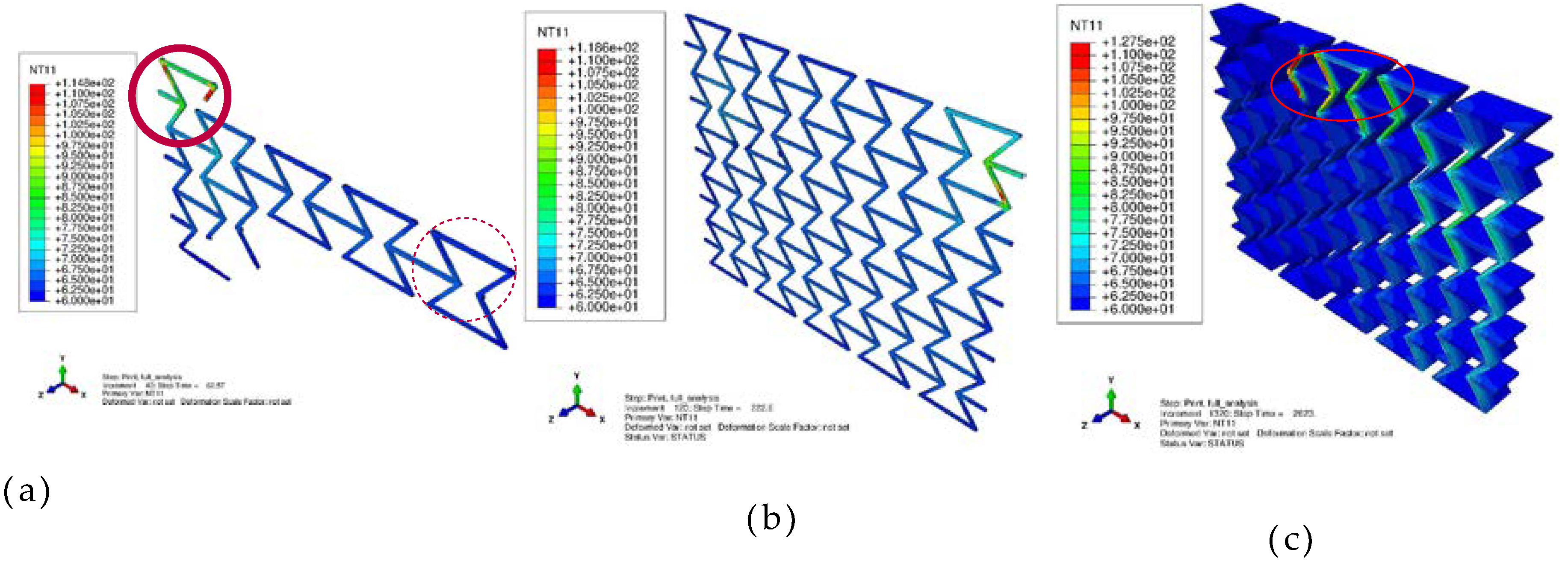
175 The printed materials experience reheating-and-cooling processes during printing, especially when additional material is deposited in the neighborhood. Fig. 5 illustrates the temperature distribution during the printing process. Fig. 5(a) presents the status during printing the first layer. Not a single layer has been completely printed yet. The solid circle marks the place where the just-printed material still shows a high temperature.
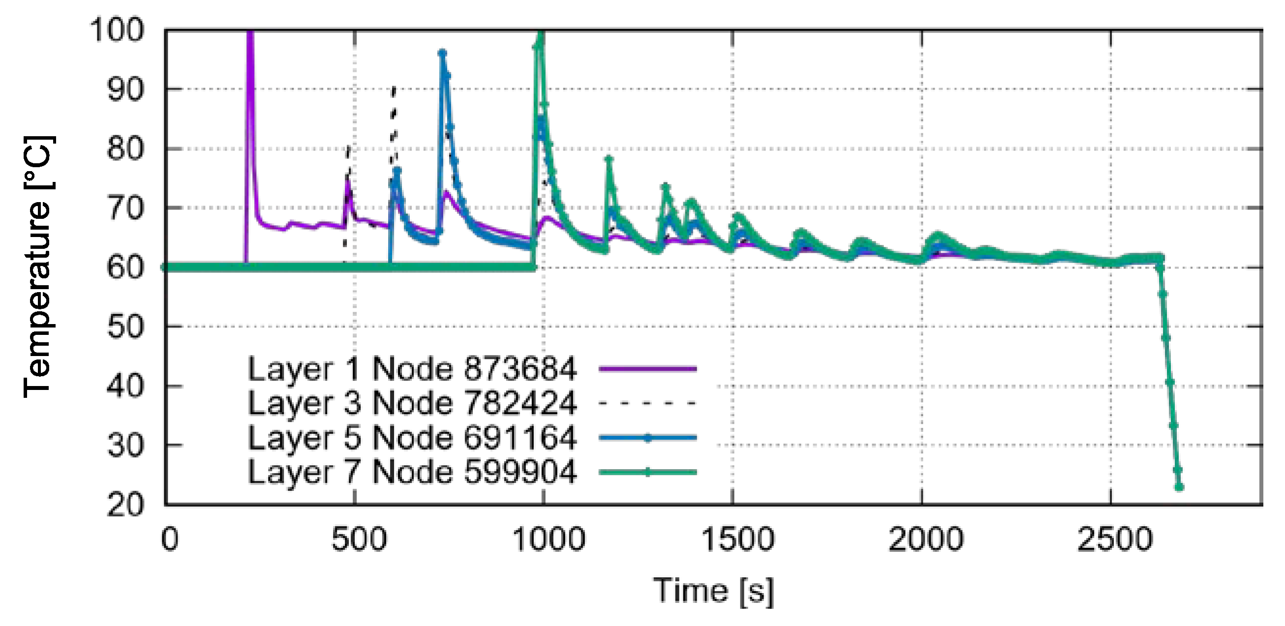
180 The material marked with the dashed circle has already cooled down to or very near to the plate temperature 60 C. Fig. 5(b) and (c) demonstrate the printed status at which the first layer or the whole structure is completely printed, respectively. As mentioned in section 3.1, the temperature is evaluated at each node in the process simulation. In order to show the temperature evolution in detail during the printing, Fig. 6 presents 185 the nodal temperature time history for four nodes, on top of the layer 1, 3, 5, and 7. The maximum temperature during printing is around 100 C. One essential factor influencing the further deformation behavior of the specimen is the RS. Its distribution is given in Fig. 7 after-cooling to room temperature.
Figure 5. Temperature distribution during the process simulation: (a) at the beginning of printing; (a) the first layer completely printed; (c) the whole structure printed.
Preprints 74253 g005
Figure 6. Nodal temperature evolution according to time for the nodes with same (X, Y) positions in different layers.
Preprints 74253 g006
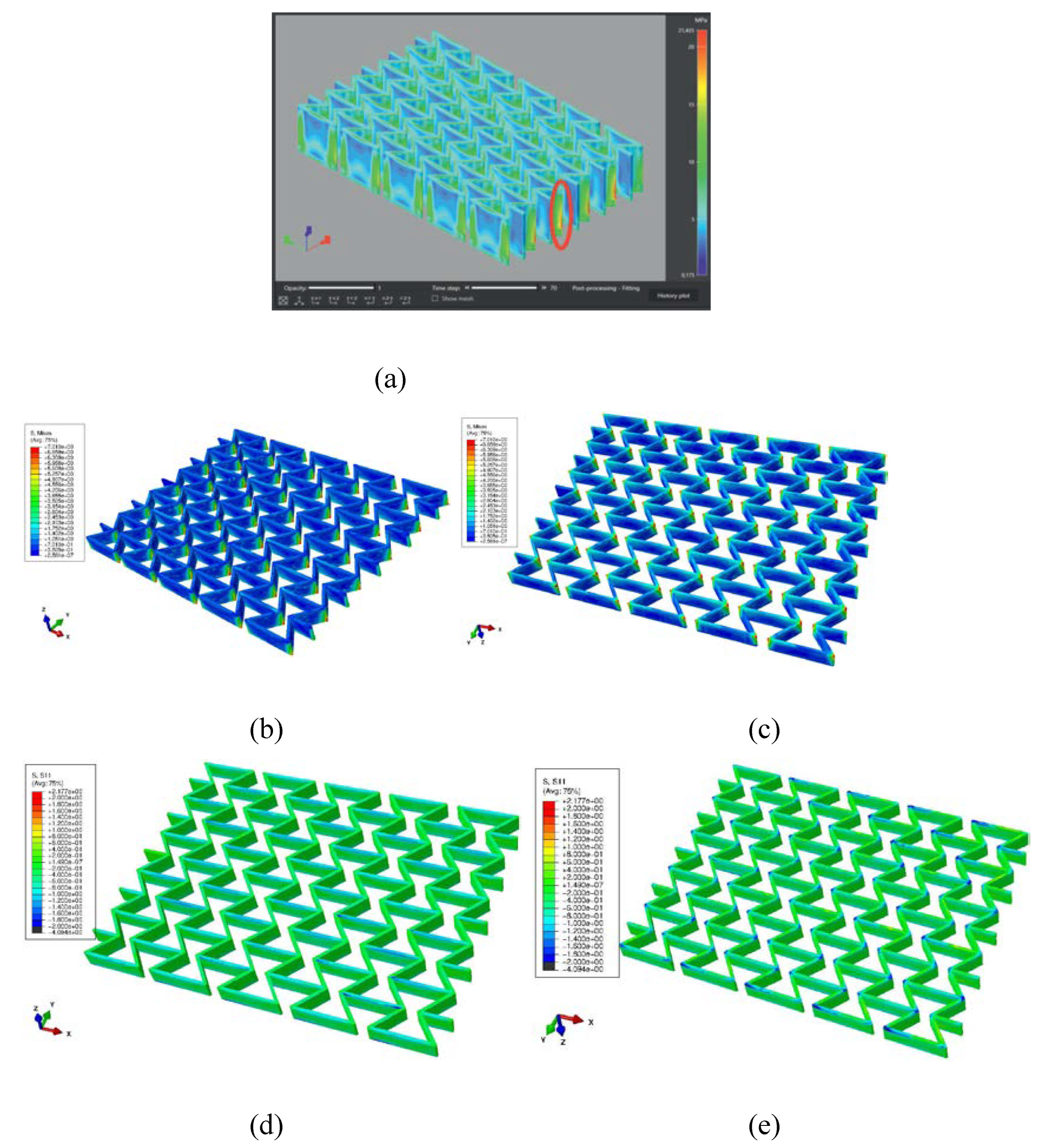
Figure 7. The process-simulation predicted RS distribution after the printing process and cooling down to room temperature: (a) using Digimat-AM [38] with ABS as the sample material; (b-e) using ABAQUS plug-in [19, 20] with PBAT, where (b-c) and (d-e) are presented as von Mises and X-direction (loading direction for further tension) stress.
Preprints 74253 g007
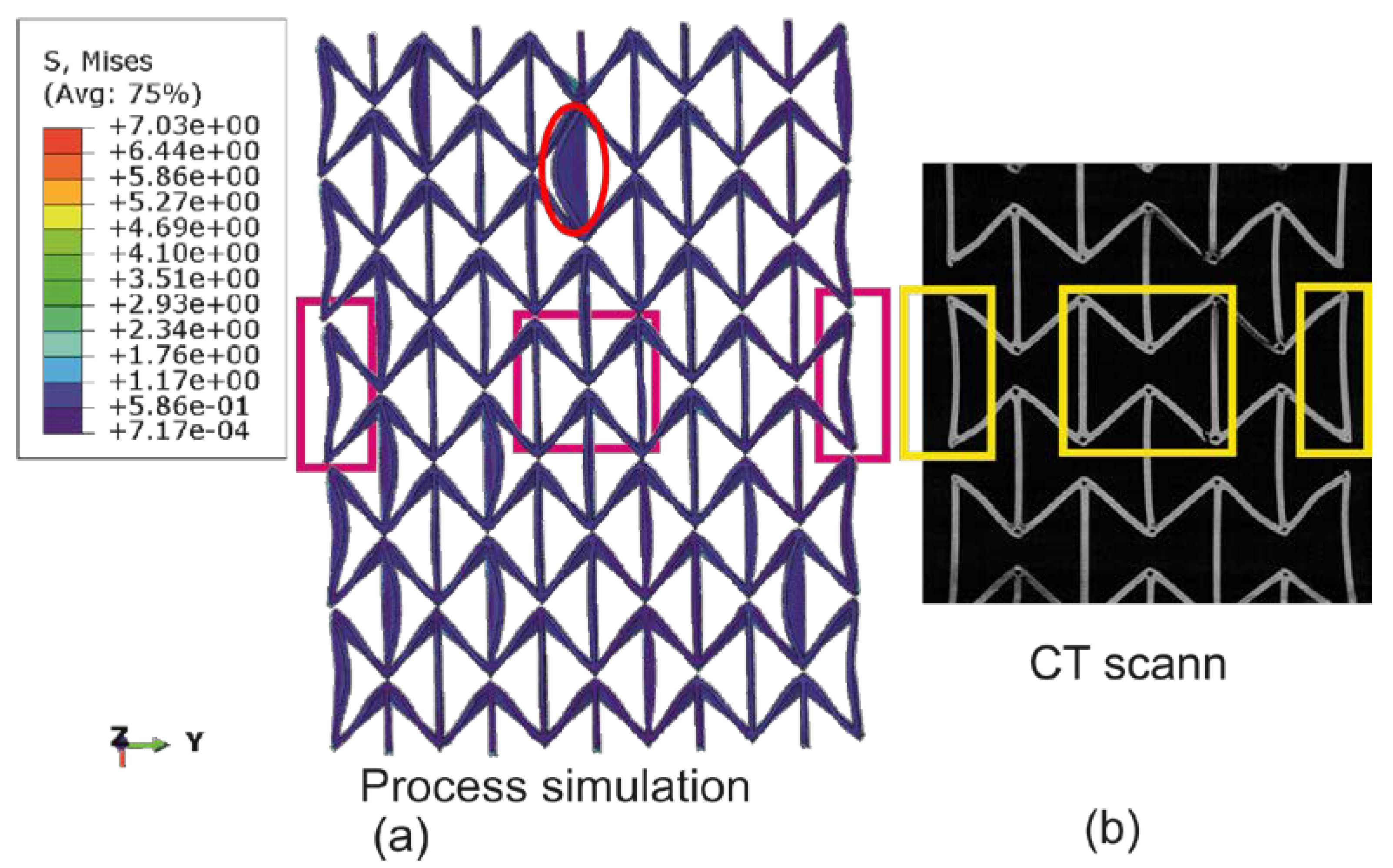
Fig. 7(a) results from another process simulation by using software Digimat-AM [38] 90 and for a sample material of acrylonitrile butadiene styrene (ABS) [39]. The oval marks the region with relatively high RSes. This subfigure is used to prove that the RS distribution predicted by using ABAQUS AM-Modeller is trustable since both types of process simulations show similar distribution patterns. Fig. 7(b)-(e) show results predicted by using ABAQUS plug-in [19, 20] for specimens made of PBAT, where (b-c) and (d-e) are 195 presented as von Mises and X-direction (loading direction in further tensile loading) stress. Fig. 8 illustrates the histogram of RSes after cooling predicted by the process simulation. Fig. 8(a) shows von Mises stress with the mean value of 0.984 MPa and (b) for stress in the X-direction with the mean value of -0.167 MPa. The repeated heating-cooling cycles in the printing process would also introduce warpages besides the RS. Fig. 9 compares 0 the warpage between the predicted and measured results, where (only) the warpage in Fig. 9(a) is the enlarged view with a deformation scale factor of five. As mentioned in section 2, the µCT test is performed on a PBAT specimen with 3 × 3 cells due to limited space in the facility. However, it is taken that the numerically predicted warpage marked in magenta rectangles and the square in Fig. 9(a) are still comparable to those marked205 in yellow in Fig. 9(b). The warpage distribution is non-homogeneous and, to show this, the red oval in Fig. 9(a) notices a strut with a relatively high warpage.
Figure 8. Histogramm of RSes after cooling predicted by the process simulation: (a) von Mises stress with the mean value of 0.984 MPa; (b) stress in the X-direction.
Preprints 74253 g008
Figure 9. Warpage comparison between experiment and simulation as inital status for tensile loading: (a) from the process simulation shown as the first printed layer on the outer side with a zoom-in factor of 5 for the warpage; (b) a selected CT scan image nearest to the surface from a sample with 3×3 cells.
Preprints 74253 g009

4.2. Numerical results predicted by mechanical simulation
The auxetic deformation behavior is studied under tension by using a structure with 5×5 cells made of PBAT. The result comparison between FE simulation (with and without 210 consideration of the RS) and experiment can deliver more detailed information about the structural deformation behavior. Furthermore, the RS influence on material behavior can be evaluated. The FE prediction without consideration of the RS is analyzed in Schneider et al. [18]. The current work presents the FE results simulated with consideration of the RS and the comparison with those without consideration of the RS.
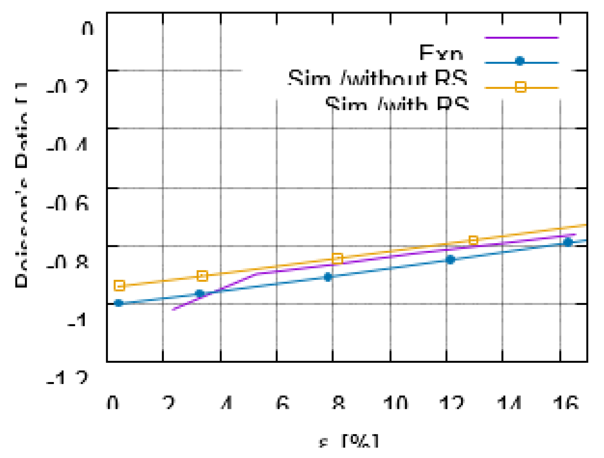
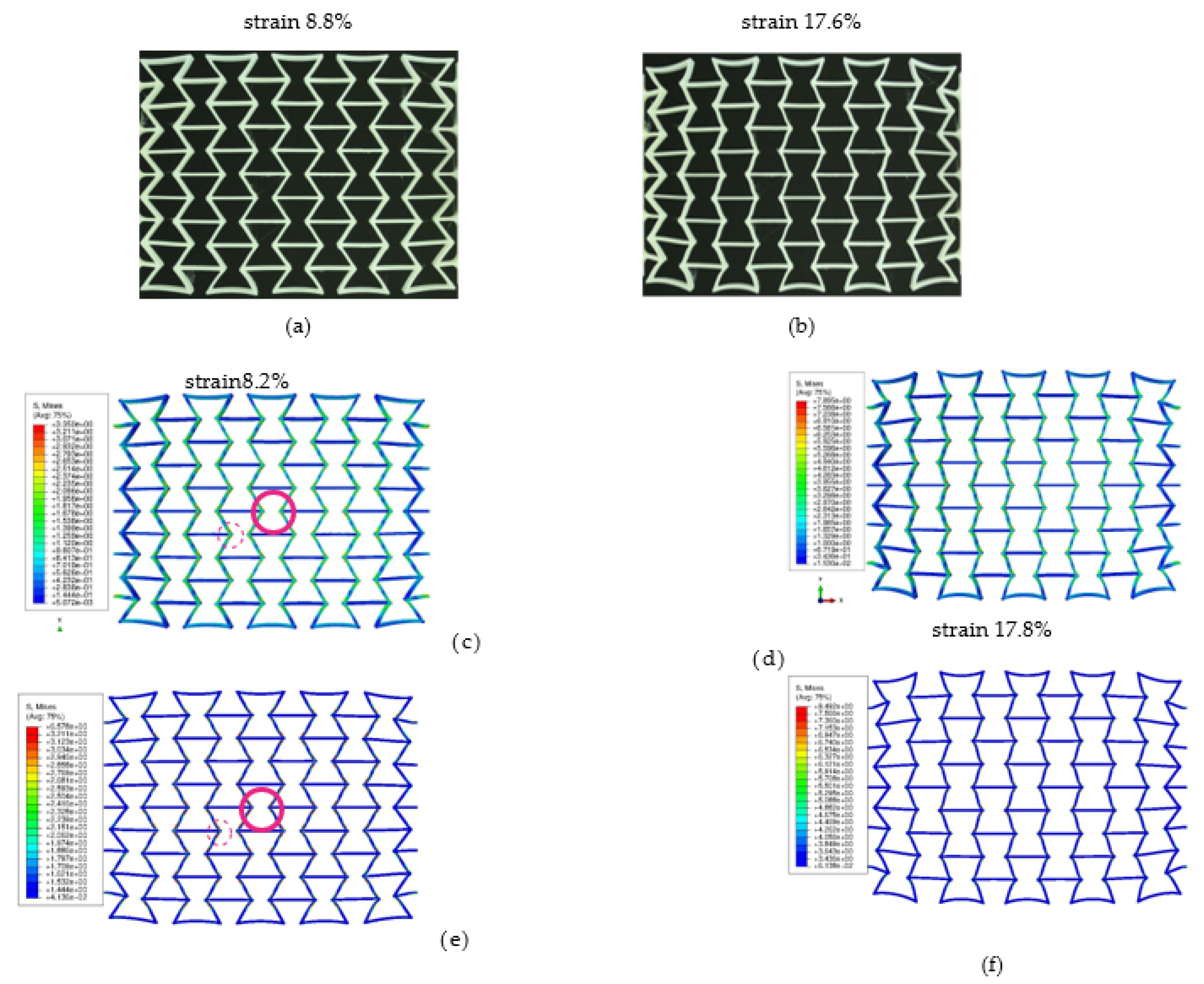
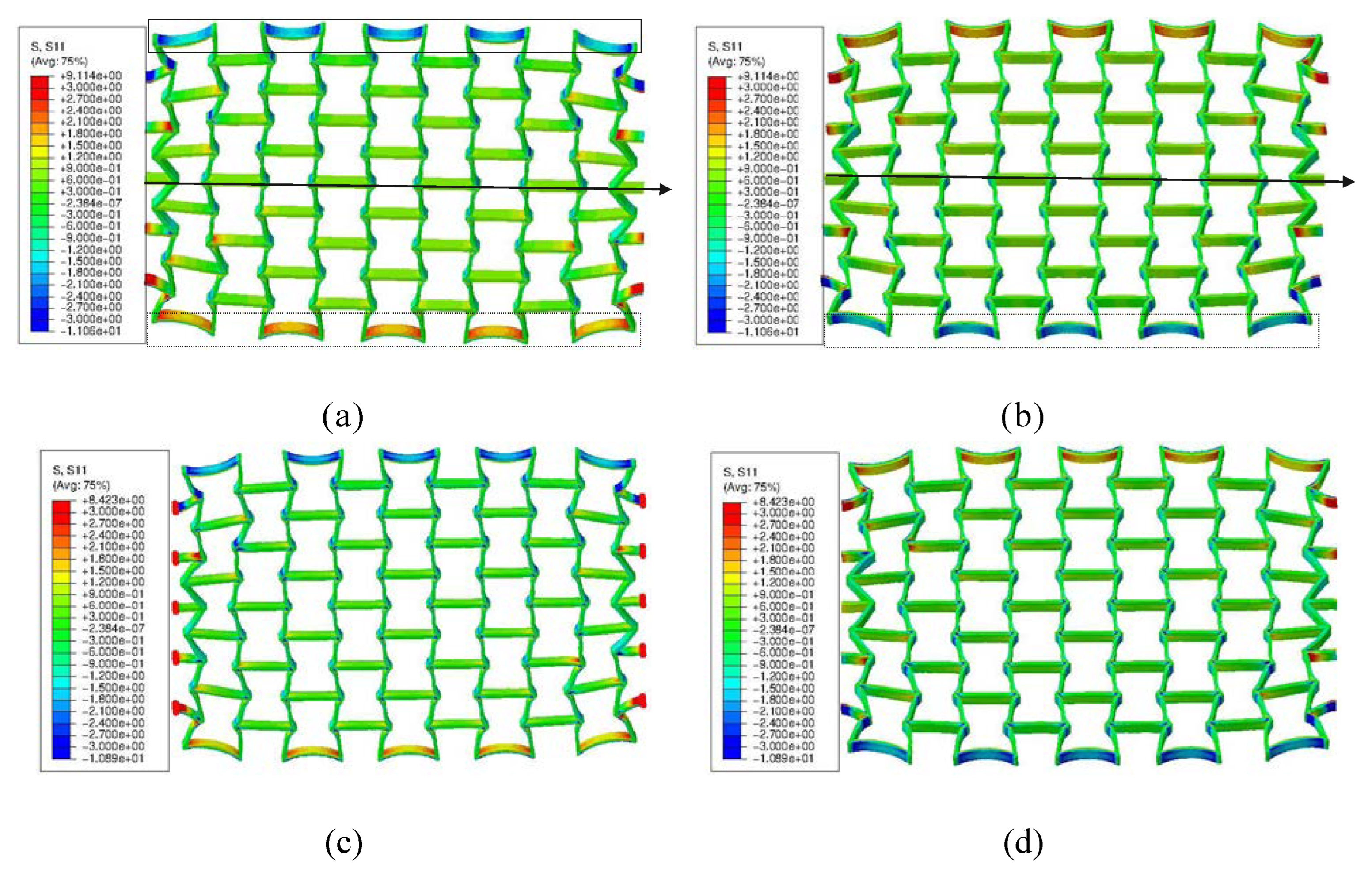
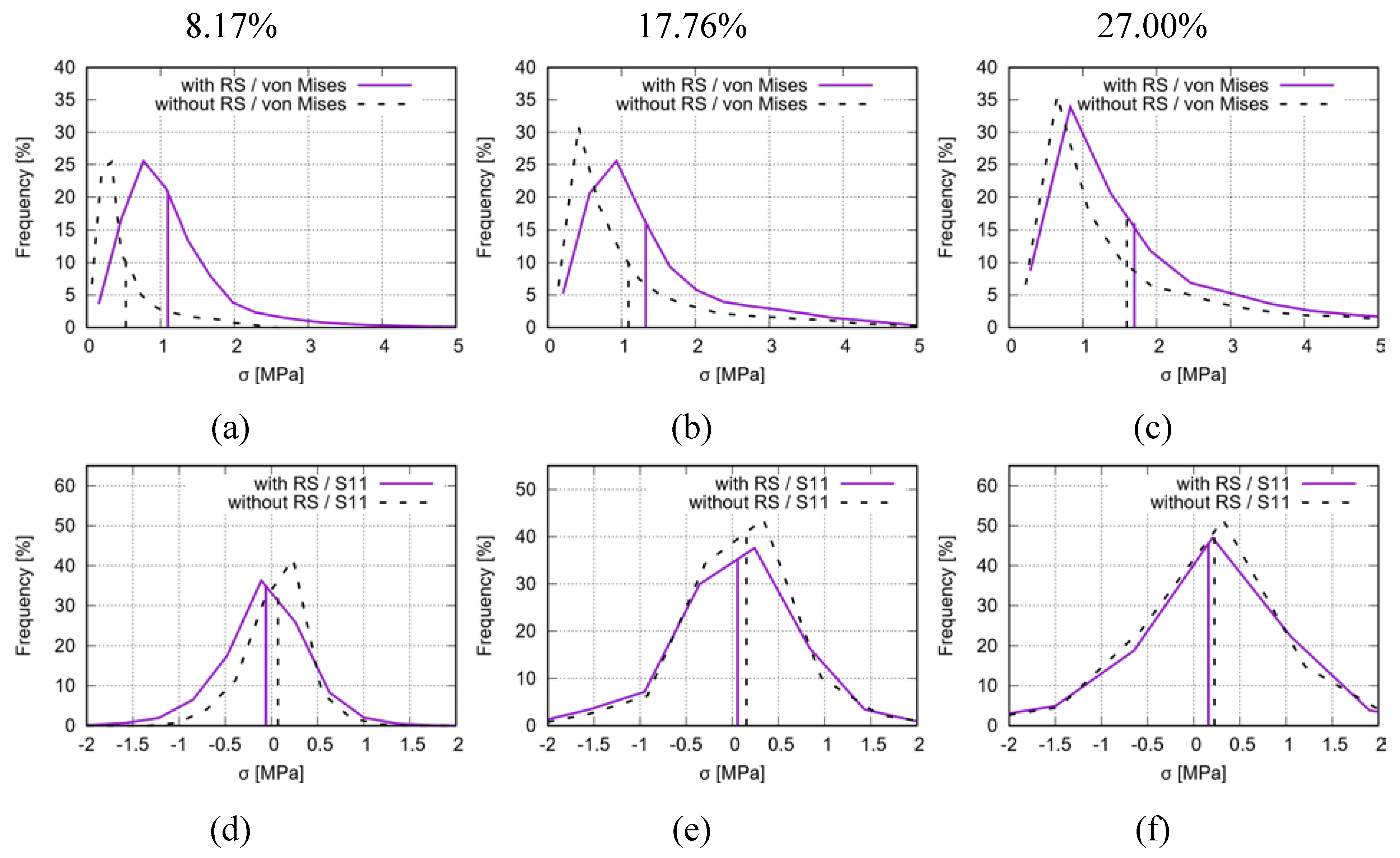
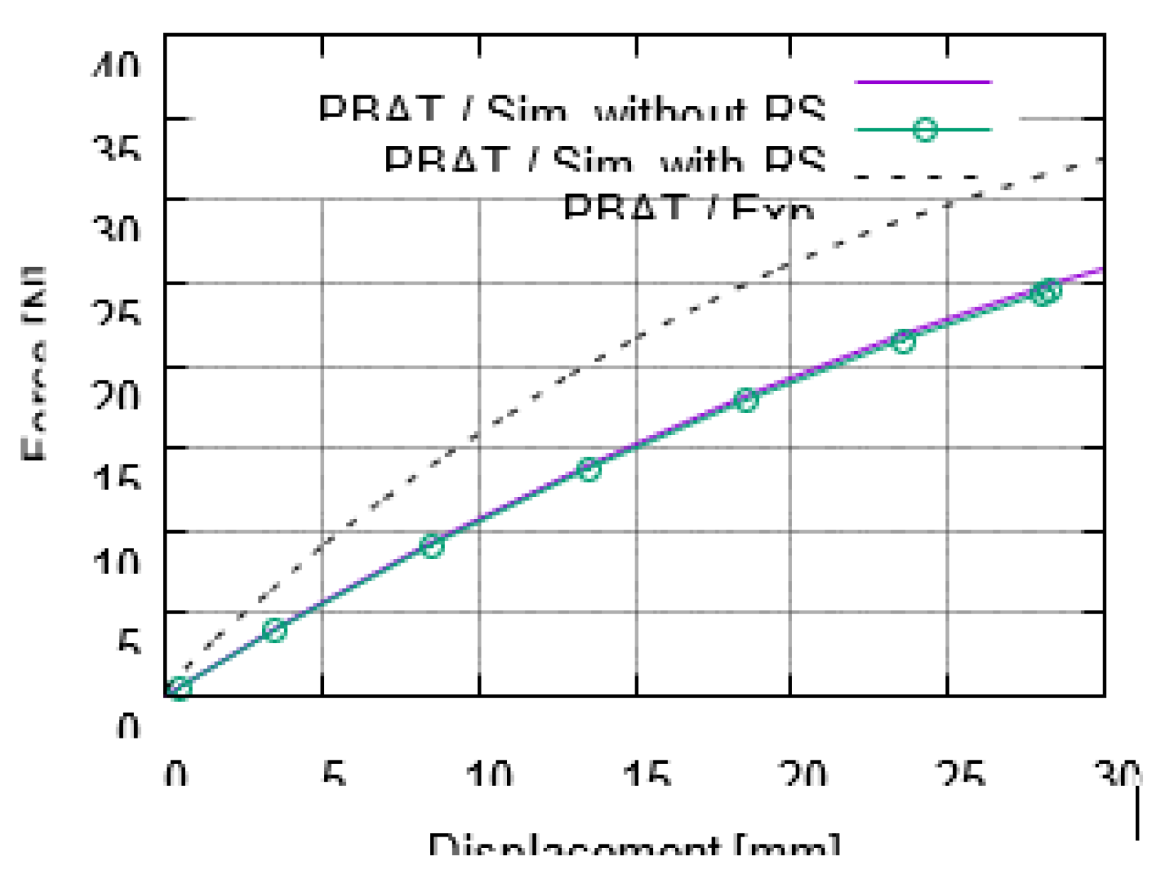
215 Fig. 10 plots the force-displacement curves from the test and from the FE prediction with and without [18] considering the RS. Fig. 11 illustrates the global stress evolution behavior according to the loading (engineering) strain. The global stress is calculated based on the elemental stresses, considering the weighting factor of the element volume fraction. Fig. 11(a) - (c) presents the evolution of the von Mises, the loading direction, and 220 the absolute value of loading direction stress. According to loading (engineering strain), Fig. 12 illustrates the structural Poisson’s ratio evolution obtained from the measurement and simulation, including with and without considering the RS for the auxetic structure with 5 × 5 cells. This calculation considers only the middle three rows for the experimental and numerical results since the auxetic deformation of the neighboring rows of clamping 225 jaws is affected by the BCs too much to show trustable auxetic behavior [18]. Fig. 13 shows the overlay view of the deformed auxetic structures from the experiment and the FE simulation, where the grey contour presents measured data and the colored area the simulated ones. The legends in Fig. 13 are only valid for the FE results. Fig. 13(a) compares the measured and FE predicted deformed status without considering the RS, 230 where the distance between the two nodes marked in red is 99.8 mm in the simulation and 100.8 mm in the experiment. For the case of FE simulation with consideration of the RS, the results are shown in Fig. 13(b) analogously. The experimentally measured and numerically predicted deformed status is given in Fig. 14 for a PBAT auxetic structure with 5×5 cells. Fig. 14(a) - (b) are measured ones at 8.8% and 17.6% loading strain, 235 respectively. Fig. 14(c) - (d) show the FE-predicted von Mises stress at 8.2% and 17.8% strain without considering RS, respectively, while (e) - (f) present FE-predicted von Mises stress at 8.2% and 17.8% strain with considering RS, respectively. Similar to von Mises stress (Fig. 14(c) - (e)), the loading direction stress distribution is plotted in Fig. 15 at different (engineering) loading status. Fig. 15(a) - (b) present the deformed status at240 27.35% strain with two perspective views, where the RS is not considered. Fig. 15(c) (d) are similar to Fig. 15(a) - (b), but with consideration of the RS. Fig. 16 illustrates the histogram of FE-predicted stress from simulations with and without consideration of RS in the deformed auxetic structure with 5 × 5 cells at various loading (engineering) strains. Fig. 16(a) - (c) show the von Mises stress at 8.17%, 17.76%, and 27% (without 245 RS 27.35%, with RS 27.07%), respectively. Fig. 16(d) - (f) are the same as (a) - (c), but for the loading direction stress.
Figure 10. Comparison of the global force-displacment curves achieved from the experiment and FE simulation including with and without [18] considering the RS for the auxetic structure with 5×5 cells made of PBAT.
Preprints 74253 g010
Figure 11. FE-predicted global stress evolution according to loading for a PBAT auxetic structure with 5×5 cells: (a) - (c) von Mises, loading direction, and the absolute value of loading direction stress, respectively.
Preprints 74253 g011
Figure 12. Comparison of the structural Poisson’s ratio evolution according to engineering strian achieved from the experiment and FE simulation including with and without [18] considering the RS for the auxetic structure with 5×5 cells made of PBAT.
Preprints 74253 g012
Figure 13. Comparison of PBAT deformed auxetic structures with 5×5 cells between experiment (gray contour) and FE simulation (colored area), where the legend only presents the FE result for the von Mises stress distribution: (a) FE simulation without RS; (b) FE simulation with RS.
Preprints 74253 g013
Figure 14. Experimentally measured and numerically predicted deformed status according to loaded engineering strain for a PBAT auxetic structure with 5×5 cells: (a)-(b) measured at 8.8% and 17.6% strain, respectively; (c)-(d) FE-predicted von Mises stress at 8.2% and 17.8% strain without considering RS, respectively; (e)-(f) FE-predicted at 8.2% and 17.8% strain considering RS, respectively.
Preprints 74253 g014
Figure 15. FE-predicted stress distribution in the loading direction for a PBAT auxetic structure with 5×5 cells: (a) - (b) without considering RS at 27.35% engineering loading strain at two different view apsect; (c) - (d) same as (c) - (b), but with considering RS at 27.07% strain.
Preprints 74253 g015
Figure 16. Histogram of FE-predicted stress from simulations with and without consideration of RSes in deformed auxetic structure with 5 × 5 cells at loading (engineering) strains: (a) - (c) von Mises stress at 8.17%, 17.76%, and 27% (without RS 27.35%, with RS 27.07%); (d) - (f) same as (a) - (c), but for loading direction stress.
Preprints 74253 g016
After this time, the entire printed auxetic structure cooled down to room temperature 23 C.
After cooling down to room temperature, no testing data is available for the residu-al stress, about which simulation can provide some basic knowledge. The FE-predicted residual stress is presented in Fig. 7 and Fig. 8 and warpage in Fig. 9.

5. Discussion

5.1. Residual stress and warpage

In the current work, the significant results from the process simulation include the 250 evolution and distribution of the nodal temperature and the RS. Here, the von Mises and the X-direction stress are presented. The X-direction corresponds to loading direction in studying the auxetic structural deformation behavior.
After being printed, a material with a small volume, presented as an element in the FE simulation, will cool down. This small volume of material will heat its neighbors at the 255 beginning of this cooling process. Furthermore, its neighbors will heat their neighbors. It leads to some regions near the just printed material (with a small volume) showing higher temperatures than other regions far away. This reheating process will be repeated due to layer-by-layer printing. From Fig. 5(a)-(c), it is evident that the places (region A) just after the printing, e.g., the region marked by a circle with a solid line in Fig.260 5(a), possess higher temperature around the melting temperature than other ones far away from region A, e.g., the region marked by a dashed circle in Fig. 5(a). Fig. 5(b) presents that the printing is simulated layer by layer, i.e., no elements in the next layer are activated before the previous layer is entirely printed. The already printed neighbors (neighboring materials) both in the same layer and underlaid layers are heated again by 265 the just printed materials, as shown in the region marked with an oval in Fig. 5(c). Due to this repeated heating, the relatively high temperature is shown in a larger region than the region covered by the just-printed material. Besides the temperature distribution, it is possible to track the node temperature evolution during the whole (pseudo) printing time (Fig. 6). Here, it is assumed that all the nodes have a temperature no less than 270 60 C since the plate’s temperature is set to be 60 C. The four selected nodes are on top of each other (similar Z coordinates according to Fig. 5). Among these selected four nodes, the node with a smaller layer number is firstly printed than the one with a higher layer number. Taking the node in the first layer as an example, its temperature evolution is shown in the purple curve in Fig. 6. It means the corresponding element is printed at 275about 240 s and has the highest temperature at this printing time point. Then, it quickly cooled down to about 68 C. Before it can further cool down, its neighboring material in the third layer is printed at the time point of about 500 s, leading to a reheating of the node in the first layer. The purple curve illustrates that a second peak appears, which is lower than the peak at the just printed status (at about 240 s). Generally, the values of 280 the following temperature peaks for a given node are gradually decreased according to its increased distance to the just printed node (element). If the current printing position is already far away from the considered node (element in the first layer), the temperature of the node in the first layer would further decrease, i.e., lower than 68 C and converging to the plate temperature 60 C. The whole printing process took 2631 s (pseudo time).
Fig. 7(a) shows the predicted RS distribution (von Mises) for ABS after the printing process and cooling down, where the software Digimat-AM is used. One characteristic of this distribution is non-homogeneous and the other is that the region marked with an oval in Fig. 7(a), the junction place of two inclined struts, possesses relatively high temperature. Still, the regions (with relatively low Z coordinate) near to the plate possess slightly 295 higher RS than those far away from the plate. One reason could be that the plate hinders the heat transfer from the printed structure to the environment. The RS distribution (von Mises) for the PBAT specimen in Fig. 7(b) is from the prediction by applying the ABAQUS plug-in AM-Modeller. Fig. 7(b) catches all the above-metioned three characteristics of the RS distribution in Fig. 7(a). It means the Digimat-AM and AM-Modeller 300 deliver the similar results. Fig. 7(c) is identical to Fig. 7(b), simply presented in another perspective view. By comparing Fig. 7(b) and (c), it is obvious that the region near to the plate owns higher RS. Fig. 7(d) and (e), results predicted by AM-Modeller, present the X-direction RS distribution at two different perspective views. Generally, both positive and negative residual stress exist in the structure for any given component in the stress 305 tensor as presented in Fig. 7(d) and (e). Fig. 8(a) and (b) illustrate the histograms of the RSes for the von Mises and the X-direction stress, respectively. The mean value of the von Mises stress (Fig. 8(a)) is about 0.984 MPa, which is very near to the expected value around 1 MPa. Theoretically, the mean value for the X-direction RS (one component of the stress tensor) should be zero, but, practically, there are always some small numerical 310 errors in FE simulations since numerical solutions are presented (no theoretical solutions are valaible). This is the reason that the mean value in Fig. 8(b) is about -0.167 MPa, but not 0 MPa.
Fig. 9 compares the predicted and measured warpage. Fig. 9(a) presents the same material status as Fig. 7(b) and (c), but with a scaling factor of five for the warpage.
The specimen with 3×3 cells, a cut view of which is shown in Fig. 9(b), possesses larger warpage than other ones. Normally, the warpage is much smaller than the one shown in Fig. 9(b). The exact reason causing the large warpage (Fig. 9(b)) is unclear. Possibly, this specimen (Fig. 9(b)) is a trial product while testing the best suitable environment for printing and cooling. However, this specimen’s in-situ µCT data enabled a good com-320 parison for the numerical prediction by chance. Another possibility is that the printing process is unstable, which causes abnormal residual stresses and warpages. Here, both the scaled warpage from the numerical result (Fig. 9(a)) and the selection of a specimen with extra large warpage (Fig. 9(b)) from the experiment aim to get the large enough deflection for the identification by naked eyes. From Fig. 9, the process simulation delivers 325 a predicted warpage well matchable to the measured ones. Such a good match is shown for the struts of cells located in the middle and on the left and right sides of the whole specimen, which are marked by rectangles in Fig. 9(a) and (b). The initially straight bars marked in rectangles (Fig. 9(b)) deformed and turned out to be arc-shaped after cooling. These phenomena are also predicted well by the FE-based process simulation (Fig. 9(a)), 330 where rectangles also mark the simulated result. Still, it is also possible that some local places possess higher warpage than others, and this phenomenon should depend on the element-activation path in the process simulation. It means the order of the activated element positions varies from layer to layer. Different activation sequences locally cause different heating-cooling cycles, leading to non-homogeneous local warpage.

5.2. Auxetic structural deformation behavior

With the numerical predicted residual stress at hand, the initial status in the FE model for simulation of the auxetic deformation behavior under tension can be set more realistically. The discussion of the tensile deformation behavior covers the global forcedisplacement curves, the global stress-strain flow behavior, the structural Poisson’s ra-340 tio evolution, the deformed status, and the stress distribution characteristics. Whenever available, the comparison is performed between experimental and numerical results. The latter includes the cases of with and without consideration of the RS. In the following, the FE model without considering the RS is called Model-NORS, and the one with Model-RS.
As mentioned, the force-displacement curve is preferred to present the macro tensile 345 deformation behavior of auxetic structures with the possibility of comparing FE and testing results. Fig. 10 illustrates the comparison of the force-displacement curves between the test and simulations with and without [18] considering the RS. Still, the FE-predicted curve considering the RS behaves minimal softer than the one without. The two curves from Model-NORS and Model-RS show a negligible slight difference. The FE-predicted 350 displacement-force curves catch the experimental flow behavior well (Fig. 10) in aspects of the non-linearity and flow behavior, even though the numerical ones behave softer than the reality at a given loading. As mentioned, the testing data of the global stress and strain is not available since the calculated stress using measured force might be too high due to the small cross-section of the auxetic structure. Otherwise, the experimental result 355 might be misleading in presenting the structural strength. In this case, the FE prediction shows superiority since the global stresses can be calculated based on elemental ones. Fig. 11 illustrates a global stress-strain curve for the PBAT specimen with 5 × 5 cells.
In Fig. 11(a), the global von Mises stress starts at 0 MPa and increases non-linearly according to the global engineering strain in the case without considering the RS. The 360 stress value reaches 1.4 - 1.6 MPa at 22.5% strain. For the simulation with RS, the initial value equals the mean value from the process simulation (Fig. 7(a), 0.984 MPa). Then, the curve shows a plateau region until about 8% strain. After that, it increases non-linearly, and the increasing ratio shows a significant discrepancy compared to the one from the FE model without considering RS. Generally, the von Mises stress level is higher 365 in the Model-RS than in the Model-NORS. However, the two curves approach each other with increasing loading, which means the RS influences the global von Mises stress at early loading more stronger than later. In reality, the warpage also has a contraction, i.e., compressive stress exits. To show this compression, the global loading direction stress is plotted in Fig. 11(b). The curve calculated from the Model-NORS starts at zero and in-370 creases nearly linearly. The curve calculated from the Model-RS starts at the mean value (-0.167 MPa, Fig. 8(b)) of the residual stress and reaches zero MPa at about 13% strain. Generally, this curve (Model-RS) increases for the whole loading range and locates lower than the curve calculated from Model-NORS. Fig. 11(c) plots the absolute value of the loading direction stress flow behavior. It means calculated curves in Fig. 11(b) and Fig.375 11(c) are based on the same original numerical data. The curve predicted by Model-RS starts at the mean value (about 0.276 MPa) of the RS for the whole auxetic structure after cooling down, and it locates above the curve predicted by the Model-NORS until about 15% loading strain. Both curves (Fig. 11(c)) increase non-linearly, especially at the beginning of loading. Then, they approach each other nearer and nearer from 10%380 strain on and meet each other at about 17% strain, from which on both curves develop nearly identically.
Fig. 12 illustrates that the Poisson’s ratio increases linearly according to loading. The value range of Poisson’s ratio presented by the experimental curve covers ≈-1 to -0.76 in the loading range of 2.3% to 16.6% (engineering strain). It means the auxetic deformation 385 ability reduces according to increasing loading strain. The Poisson’s value of -0.76 at about 16.6% loading strain indicates that the structure still possesses an excellent auxetic deformation potential since this value is still much lower than zero. The comparison of the measured and predicted Poisson’s ratio evolution of the auxetic structure (Fig. 12) shows that the numerical curves of both FE models (Model-NORS and Model-RS) capture 390 the experimental one well for both the linearity and the value range. The numerical curve predicted by the Model-NORS locates slightly lower than the experimental curve. It means the prediction presents a better auxetic behavior than the reality since the values in this FE curve are nearer to the optimum value of -1. Since the other FE curve (from Model-RS) is located above the FE curve (from Model-NORS) and nearly at the same position as the 395 measured curve, the RS improves the numerical prediction. It also implies that the RS negatively influences the auxetic deformation behavior. A further numerical investigation is necessary to map the higher gradient in the experiment in the loading range of about 2.3% to 5%. The speculation is that this higher ratio is geometric parameters of the auxetic structure dependent, and the current FE simulation did not include such parameters in 400 the material model (theory).
The deformed topologies predicted by the Model-NORS and the Model-RS at about 12% loading (engineering) strain are very similar since both FE results match the measured one very well (Fig. 13). However, the stress range from the Model-RS (Fig. 13, right) covers a larger distance than the one from the Model-NORS (Fig. 13, left). It405 means the RS obviously influences the stress magnitude and distribution but not much of the deformed topology. Concerning the auxetic behavior, the results from both cases prove that the two rows as neighbors of clamping jaws should be excluded in calculating the Poisson’s ratio or analyzing the auxetic structural deformation behavior since the deformation of cells in these two rows is strongly influenced by the BCs. Such cells’ 410 deformation is not the same as those in other rows. For a more detailed discussion about the deformed status, it might refer to Schneider et al. [18].
Fig. 14 compares further deformed status of the tested (Fig. 14(a)-(b)) and FEpredicted (Fig. 14(c)-(f)) auxetic structures. The latter (Fig. 14(c)-(f)) also illustrates the von Mises stress distribution and its covered value range. The FE prediction of both 415 Model-NORS and Model-RS matches the experimental topological deformation characteristics well. Similar to the results shown in Fig. 13, cells in the middle three rows deform less than those at the end rows. The struts of each cell on structural free edges (e.g., left and right rows in Fig. 14(c)) experience higher deformation than the other struts.
The major reason should be the BCs. The first type of struts mentioned above is free of 420 constraints from neighboring cells. The cells as neighbors of the clamping jaw deformed much, where the rotation and the distortion are apparent. At about 8% loading strain, the stress range is about (0, 3.35) MPa predicted by the Model-NORS (Fig. 14(c)), while it is about (0, 6.58) MPa by the Model-RS (Fig. 14(e)). At about 17.5%, the maximum stress values are about 7.89 and 9.49 MPa in the Model-NORS and the Model-RS, respective425 ly. The stress difference in the two FE models decreases according to increasing loading. It implies that the residual stress influences the structural stress more obviously in the early loading stage. Still, joining positions of horizontal and inclined struts (region-tip), e.g., denoted in magenta circles (Fig. 14(c) and (e)), present relatively high stress in the whole structure and for both cases. Here, regions with high stress and with high strain are 430 coincident. Due to geometrical factors, the strain gradient at such places is high, which results in high strain values. Comparing Fig. 14(c) to (e) and Fig. 14(d) to (f), another characteristic is that the stress distribution in Model-RS (Fig. 14(e) and (f)) shows higher local concentration than the one in Model-NORS (Fig. 14(c) and (d)). Most regions in the former (Fig. 14(e) and (f)) show blue color (very low stress) and small areas near 435 to region-tip present high-stress values (red color). However, in the latter (Fig. 14(c) and (d)), blue regions (with low-stress values) are much less than in the former. Still, the green-yellow regions (with intermediate stress values) exit. The large local discrepancy of the stress distribution negatively influences the structural loading burden capacity, which leads to the assumption that the specimen with RS would first break compared to the one 440 without. In reality, it can be taken that the specimen with larger residual stress would be broken earlier than the one with less since every specimen is expected with RS. Another characteristic of deformation and stress distribution is that both deformation and stress distribution is approximately symmetric according to the geometrical middle line of the specimen in the tension direction. It is more apparently shown in Fig. 15. The loading 445 direction stress distribution in Fig. 15(a) and (b) (Model-NORS) is identical, simply shown in different perspective views. The upper struts marked in the solid rectangle and the lower struts marked in the dashed rectangle show symmetric deformation according to the marked arrow (Fig. 15). The stress distribution on the outside surface in the upper struts (marked in solid rectangle in Fig. 15(a)) is almost the same as the one on the 450 outer surface in the lower struts (marked in the dashed rectangle in Fig. 15(b)). The same deformation and stress distribution characteristic is also presented by the Model-RS (Fig. 15(b)(d)). From all the four images in Fig. 15, a further conclusion is that the struts connecting the clamping jaw, ends of which are denoted with red points in Fig. 15(c), are critical regions which possess both large deformation and high stress. 455 Concerning the conclusion that the RS influence on the stress distribution decreases, it is more evident from the histograms of von Mises and loading direction stresses shown in Fig. 16. The discrepancy for both the curve position and the mean value of the von Mises stress between the results predicted by the Model-NORS and the Model-RS (Fig. 16(a)-(c)) reduces according to loading. The discrepancy caused by RS and its reduction means 460 the less-and-less effect of RS on the stress in the structure. The mean values of the von Mises stress of the whole auxetic structure are 0.53, 1.01, and 1.60 MPa at 8.17%, 17.76%, and 27.35% loading (engineering) strain from the Model-NORS, while these three values are 1.10, 1.33 and 1.70 MPa (1.70 MPa at 27.07% strain) from the Model-RS. Recalling the RS stress value 0.918 MPa (von Mises) at the beginning of the loading, its effect 465 is gradually minimized for the structural stress values, but its influence on the stress distribution pattern remains (comparing Fig. 14(d) and (f)), at least the effect vanishing not as quick as for the stress value. Analogously, Fig. 16(d)-(f) present the results for the loading direction stress and show similar characteristics as in Fig. 16(a)-(c), but with a smaller discrepancy for the curve position and the stress value.

6. Conclusion

The current work investigates the tensile deformation behavior of auxetic structures made of PBAT polymers and emphasizes the RS’s influence on the deformation behavior. The FE-based process simulation predicts the warpage and the RS. The reconstructed auxetic structure from µCT images calibrates the predicted warpage. Since the predicted 475 warpage is negligibly small, it is not considered in the further FE calculation. Testing data are unavailable for the RS. The numerical RS serves as the initial condition for the FE model under tension. The FE results from the models with and without considering the RS are compared. When testing data are available, the comparison is also made between FE simulation and experiment. It leads to the following conclusions:
  • FE-based process simulation:
-
After cooling down, the junction places of the two inclined struts present higher residual stress than other places in the cell.
-
After cooling down, the inhomogeneous warpage among cells or inside one cell is well predicted compared to the µCT measured real specimen.
-
The histogram shows a mean value of the RS, taking von Mises stress as an indicating factor, slightly less than 1 MPa, which can be served as a reference value in estimating the real residual stress.
  • Auxetic structural tensile deformation:
-
The force-displacement curve predicted by the FE model considering the RS 490 shows negligible softer behavior compared to the one without. Both FE curves capture the highly non-linear and evolution behavior of the experimental one, where the numerical result behaves softer than reality.
-
At the beginning of loading, the RS illustrates a stronger influence on the global stresses (von Mises stress and stress in the loading direction) of the 495 auxetic structure. From about 15% global (engineering) strain on, the global stresses predicted by FE models with and without RS approach to each other.
-
The Poisson’s ratio evolution predicted by both FE models matches the experimental result very well for the auxetic structure. The FE model, with consideration of the RS, presents an even better mapping of the experimental 500 one.
-
The RS affects the topological deformation much less than the stress value and distribution. By overlapping the deformed status of the auxetic structure from the test and the FE calculation, it shows that both FE models can predict the real auxetic deformation characteristics in detail.
-
The FE results predicted by both models show that the deformation and stress distribution present symmetric behavior according to the geometric middle line paralleling the loading direction.
-
Generally, RS negatively affects the auxetic deformation behavior.

Author Contributions

conceptualization Y.S., V.G., S.S.; methodology Y.S., V.G., 510 S.S., J.K.; experiment and data collection J.H., A.G., C.B.; thesis supervision Y.S., V.G.; FE simulation Y.S., V.G., A.S.; writing—original draft preparation Y.S., V.G.; review and editing all authors. All authors have read and agreed to the submitted version of the manuscript.

Funding

This work was supported by the German Scientific Foundation (DFG) [grant numbers of SCHM 746/221-1 and BO 1600/51-1].

Data Availability Statement

Data is contained within the manuscript.

References

  1. K. E. Evans, Auxetic polymers: a new range of materials, Endeavour 15 (4) (1991) 170–174 (1991). [CrossRef]
  2. K. Wojciechowski, Remarks on “Poisson ratio beyond the limits of the elasticity theory”, Journal of the Physical Society of Japan 72 (7) (2003) 1819–1820 (2003). [CrossRef]
  3. X. Ren, R. Das, P. Tran, T. Ngo, Y. Xie, Auxetic metamaterials and structures: a 525 review, Smart Mater. Struct. 27 (23001) (2018). [CrossRef]
  4. J. Grima, R. Gatt, Perforated sheets exhibiting negative Poisson’s ratios, Advanced Engineering Materials 12 (2010) 460–464 (2010). [CrossRef]
  5. R. Almgren, An isotropic three-dimensional structure with Poisson’s ratio=-1, Journal of Elasticity 15 (1985) 427–430 (1985). [CrossRef]
  6. L. Ai, X.-L. Gao, Metamaterials with negative Poisson’s ratio and nonpositive thermal expansion, Composite Structures 162 (2017) 70–84 (2017). [CrossRef]
  7. S. Pandini, A. Pegoretti, Time and temperature effects on Poisson’s ratio of poly(butylene terephthalate, eXPRESS Polymer Letters 5 (8) (2011) 685–697 (2011). [CrossRef]
  8. L. J. Gibson, M. Ashby, G. S. Schajer, C. I. Robertson, The mechanics of twodimensional cellular materials, Proceedings of the Royal Society of London. A. 382 (1982) 25–42 (1982). [CrossRef]
  9. C. Mercer, T. Speck, J. Lee, D. S. Balint, M. Thielen, Effects of geome-540 try and boundary constraint on the stiffness and negative Poisson’s ratio behaviour of auxetic metamaterials under quasi-static and impact loading, International Journal of Impact Engineering 169 (104315) (2021) 1–12 (2021). [CrossRef]
  10. T. Masselter, G. Bold, M. Thielen, O. Speck, T. Speck, Bioinspired materials and 545 structures: A case study based on selected examples, in: G. Yang, L. Xiao, L. Lamboni (Eds.), Bioinspired Materials Science and Engineering, Wiley, Wuhan, 2018, pp. 251– 266 (2018). [CrossRef]
  11. Buhrig-Polaczek,¨ C. Fleck, T. Speck, P. Schuler,¨ S. Fischer, M. Caliaro, M. Thielen, Biomimetic cellular metals-using hierarchical structuring 550 for energy absorption, Bioinspir Biomim 11 (4) (2016) 045002 (2016). [CrossRef]
  12. S. Choi, Z. Ku, S. Kim, K. Choi, A. Urbas, Y. Kim, Silk is a natural metamaterial for self-cooling: An oxymoron?, in: 2018 Conference on Lasers and Electro-Optics (CLEO), 2018, pp. 1–2 (2018).
  13. P. U. Kelkar, H. S. Kim, K.-H. Cho, J. Y. Kwak, C.-Y. Kang, H.-C. Song, Cellular auxetic structures for mechanical metamaterials: A review, Sensors 20 (3132) (2020) 1–26 (2020). [CrossRef]
  14. R. Negrea, Brief review of metamaterials and auxetic materials, Automotive Series XXVII (31) (2021) 1–9 (2021). [CrossRef]
  15. T. D. Ngo, A. Kashani, G. Imbalzano, K. T. Nguyen, D. Hui, Additive manufacturing (3D printing): A review of materials, methods, applications and challenges, Composites Part B: Engineering 143 (2018) 172–196 (2018). [CrossRef]
  16. B. Praveena, N. Lokesh, B. Abdulrajak, N. Santhosh, B. Praveena, R. Vignesh, A 565 comprehensive review of emerging additive manufacturing (3D printing technology): Methods, materials, applications, challenges, trends and future potential, Materials Today: Proceedings 52 (2022) 1309–1313, international Conference on Smart and Sustainable Developments in Materials, Manufacturing and Energy Engineering (2022. [CrossRef]
  17. M. Manoj Prabhakar, A. Saravanan, A. Haiter Lenin, I. Jerin Leno, K. Mayandi, P. Sethu Ramalingam, A short review on 3D printing methods, process parameters and materials, Materials Today: Proceedings 45 (2021) 6108–6114, international Conference on Mechanical, Electronics and Computer Engineering 2020: Materials Science (2021). [CrossRef]
  18. Y. Schneider, V. Guski, S. Schmauder, J. Kadkhodapour, J. Hufert, A. Grebhardt, C. Bonten, Deformation behavior investigation of auxetic structure made of poly(butylene adipate-co-terephthalate) biopolymers using finite element method, Polymers 15 (7) (2023) 1–23 (2023). [CrossRef]
  19. ABAQUS/Standard, Hibbitt, Karlsson & Sorensen, Inc., 2020 (2020). ABAQUS, AM Modeler (2020)Download link: https://github.com/Dr-Ning-An/ebmabaqus.
  20. J. Hufert, A. Grebhardt, Y. Schneider, C. Bonten, S. Schmauder, Deformation behavior of 3D printed auxetic structures of thermoplast polyermers: PLA, PBAT, and blends, Polymers 15 (2) (2023). [CrossRef]
  21. J. Jiao, X. Zeng, X. Huang, An overview on synthesis, properties and applications of poly(butylene-adipate-co-terephthalate)–PBAT, Advanced Industrial and Engineering Polymer Research 3 (2020) 19–26 (2020). [CrossRef]
  22. B. Liu, T. Guan, G. Wu, Y. Fu, Y. Weng, Biodegradation behavior of degradable mulch with poly (butylene adipate-co-terephthalate) (PBAT) and poly (butylene 590 succinate) (PBS) in simulation marine environment, Polymers 14 (8) (2022) 1515–1– 12 (2022). [CrossRef]
  23. F. Ferreira, L. Cividanes, R. Gouveia, L. Lona, An overview on properties and applications of poly(butylene adipate-co-terephthalate)– PBAT based composites, Polymer Engineering and Science 59 (2019). [CrossRef]
  24. L. Jiang, M. P. Wolcott, J. Zhang, Study of biodegradable polylactide/poly(butylene adipate-co-terephthalate) blends, Biomacromelecules 7 (2006) 199–207 (2006). [CrossRef]
  25. M. Mori, A. Hansel, M. Fujishima, Machine Tool, Springer Berlin Heidelberg, Berlin, Heidelberg, 2014, pp. 792–801 (2014). [CrossRef]
  26. V. Pavelic, R. Tanbakuchi, P. S. Uyehara, A. O. und Myers, Experimental and computed temperature histories in gas tungsten arc welding of thin plates, Welding Journal Research Supplement 48 (1969) 296–305 (1969).
  27. N. Pierron, P. Sallamand, J. M. Jouvard, E. Cicala, S. Matte¨ı, Determination of an empirical law of aluminium and magnesium alloys absorption coefficient during Nd:.
  28. YAG laser interaction, Journal of Physics D: Applied Physics 40 (2007) 2096–2101 (2007). [CrossRef]
  29. Gibson, D. Rosen, B. Stucker, M. Khorasani, Material extrusion, in: Additive Manufacturing Technologies, in Additive Manufacturing Technologies, Springer International Publishing, Cham, 2021, pp. 171–201 (2021). [CrossRef]
  30. Q. Sun, Z. Shan, L. Zhan, S. Wang, X. Liu, Z. Li, S. Wu, Warp deformation model of polyetheretherketone composites reinforced with carbon fibers in additive manufacturing, Materials Research Express 8 (12) (2021) 125305 (2021). [CrossRef]
  31. N. An, G. Yang, K. Yang, J. Wang, M. Li, J. Zhou, Implementation of abaqus usersubroutines and plugin for thermal analysis of powder-bed electron-beam-melting additive manufacturing process, Materials Today Communications 27 (2021) 102307 (2021). [CrossRef]
  32. BASF (2013) 1–3Last visit May 03, 2022 (2013). [link]. URL https://documents.basf.com/c32f5c099d8e29ac42869b975517bdbdda6e62f4/ecoflex_F.
  33. Z. Ali, H. Youssef, H. M. Said, H. Saleh, Thermal stability of LDPE, iPP and their blends, Thermochimica Acta 438 (1) (2005) 70–75 (2005). [CrossRef]
  34. M. Ta¸sdemir, H. Biltekin, G. T. Caneba, Preparation and characterization of ldpe and 625 pp-wood fiber composites, Journal of Applied Polymer Science 112 (2009) 3095–3102 (2009). [CrossRef]
  35. M. Bednarik, D. Manas, M. Manas, A. Mizera, M. Reznicek, Effect of ionizing beta radiation on the mechanical properties of poly(ethylene) under thermal stress, MATEC Web of Conferences 76 (02019) (2016) 1–4 (2016). [CrossRef]
  36. ABAQUS/Standard, Hibbitt, Karlsson & Sorensen, Inc., 2018 (2018).
  37. O. Sahin, Finite element simulations of additively manufactured PBAT polymer with auxetic behavior in 2D and 3D (2022).
  38. Digimat AM, last visit Nov. 17, 2022 (2019).
  39. C. Hou, Numerical investigations on additive manufacturing of metamaterials with 2d structure (2020).
Disclaimer/Publisher’s Note: The statements, opinions and data contained in all publications are solely those of the individual author(s) and contributor(s) and not of MDPI and/or the editor(s). MDPI and/or the editor(s) disclaim responsibility for any injury to people or property resulting from any ideas, methods, instructions or products referred to in the content.
Copyright: This open access article is published under a Creative Commons CC BY 4.0 license, which permit the free download, distribution, and reuse, provided that the author and preprint are cited in any reuse.
Prerpints.org logo

Preprints.org is a free preprint server supported by MDPI in Basel, Switzerland.

Subscribe

© 2024 MDPI (Basel, Switzerland) unless otherwise stated