Preprint
Article

Wideband DOA Estimation Utilizing Hierarchical Prior Based on Variational Bayesian Inference

Altmetrics

Downloads

112

Views

26

Comments

0

Submitted:

12 May 2023

Posted:

23 May 2023

You are already at the latest version

Alerts
Abstract
Sparse direction-of-arrival (DOA) estimation of wideband signal has attracted widespread researches for its unique high-resolution performance. Numerous existing methods based on sparse Bayesian learning (SBL) don’t possess the ability to enhance sparsity even if they have already enjoyed high favor among sparse recovery approaches. In view of this, we propose a novel hierarchical Bayesian prior framework that enhance sparsity evidently and derive its corresponding iterative algorithm. On analysis, the computational complexity of the iterative are less than most existing other state-of-the-art algorithms. Not only that, proposed method possesses high angular estimation precision and sparsity performance by utilizing joint sparsity of multiple measure vector (MMV) models. Last but not least, the method obtains the ability to stabilize the estimated values between different frequencies or snapshots such that flat spatial spectrum. Extensive simulation results are presented to prove the superior performance of our methods
Keywords: 
Subject: Physical Sciences  -   Other

1. Introduction

DOA estimation is an important research focus that has developed rapidly during the past three decades in array signal processing, and its applications are spread across military and civilian fields such as radar, sonar, wireless detection, mobile communication, and biomedicine [1]. It is a remarkable fact that most current researches are based on narrowband signal, while the study for wideband-signal DOA estimation is of equal importance since the common assumption that signals incident from different angles occupy the same frequency band does not always hold in practice [2,3]. In addition, compared to narrowband signals, band signals are characterized by high resolution, which means higher estimation accuracy and better robustness to correlated sources.
Traditional DOA estimation methods for wideband signals can be roughly divided into two categories, one is incoherent signal subspace methods (ISSM) [4,5] and the other is coherent signal subspace methods (CSSM) [6,7,8]. The common point between them is to convert no-spectrum-aliasing wideband signals into narrowband signals for processing, while the most obvious difference is that CSSM can handle coherent sources with lower operational complexity. It is worth noting that there are two methods based on orthogonal testing between ISSM and CSSM, though some literature classifies them as special ISSM category. One is the test of orthogonality of projected subspaces (TOPS), the other is the test of orthogonality of frequency subspaces (TOFS). TOPS and TOFS are with different principles such that they place different emphasis on DOA estimation problems. Their common features are that they can solve the problem of seeking the optimal reference frequency point, and find a balance between the signal to noise ratio (SNR) and the computational complexity. However, all of them need to face the following basic limitations: (ⅰ) Most of them need pre-estimation procedure. (ⅱ) The relatively higher snapshot accumulation is necessary for accurate angular estimation. (ⅲ) A priori of the number of sources is required. (ⅳ) Most of their performance is constrained by the SNR.
For aforementioned limitations, many algorithms based on compressed sensing and sparse representation have been proposed and gradually developed [9,10]. These methods possess better performance than traditional ones such as locating coherent sources well, depending less on high SNR and snapshots and operating with higher efficiency. According to the current research, the methods based on sparse representation for wideband-signal DOA estimation can be broadly classified into three categories: the first one is based on basis pursuit, such as matching pursuit (MP) [11] and orthogonal matching pursuit (OMP) [12]; the second one is based on convex optimization, such as JLZA [13], l 1 -SVD [14] and W-SpSF [15]; the final one is based on Bayesian compressed sensing [16,17]. The methods’ comprehensive performance of sparse Bayesian learning (SBL) is reported to be better than that based on basis pursuit or convex optimization, though this conclusion was drawn by narrowband signals [18]. There exist several methods based on sparse Bayesian learning, but they all adopted single measure vector model (SMV) [17] or generalized SMV model [16]. In other words, these methods aim at single-snapshot models or vectorized multiple-snapshot models, which would result in a simple decoupling between snapshots. In fact, a reasonable use of temporal correlation not only represents the time-domain coherence of sources, but also improves the algorithm performance. In conclusion, it has been shown that the MMV model has better properties than the SMV model (e.g., stronger joint sparsity and better sparse recovery) [19,20].
In view of this, a novel method, based on the block sparse Bayesian model for wideband-signal DOA estimation, is developed in this paper. The method can be considered as one extension of the SBL based on the SMV model to the MMV model, or as the other extension of the SBL based on narrowband DOA estimation to wideband-signal one. On the basis of SBL, the method takes full advantage of the MMV model by transforming the MMV model into block-sparse model. Not only that, the tactfully design for proposed algorithm allows the joint sparsity between snapshot and spectrum to be exploited simultaneously. In addition, compared to the traditional Gaussian prior, the employed hierarchical structure of the prior can greatly improve the induced sparsity of sparse Bayesian learning.
The rest of this work is organized as follows. In Section 2, the data model is introduced and transformed. In Section 3, the likelihood and prior are presented for variational Bayesian inference and computational complexity of various approaches are compared. The performance of our algorithms is evaluated in Section 4 and the conclusions are drawn in Section 5.

2. Data model

Assume K uncorrelated far-field wideband sources from different directions θ = { θ 1 , ... , θ K } impinge on a linear array with N sensors. Without loss of generality, corresponding received data is modeled as
x ( t ) = A s ( t ) + n ( t )
where A = [ a ( θ 1 ) , ... , a ( θ K ) ] N × K is array manifold matrix with its k t h entry is a ( θ k ) = [ exp ( j v 1 ) , ... exp ( j v N ) ] T , v n = 2 π f d n sin ( θ k ) / c , n = 1 , ... , N . d n denotes the location of the n t h sensor relative to reference one, c is propagation velocity. s ( t ) = [ s 1 ( t ) , ... , s K ( t ) ] and n ( t ) = [ n 1 ( t ) , ... , n N ( t ) ] are signal waveform vector and additive white Gaussian noise (AWGN) vector, respectively. Then the time-domain data could be converted into frequency-domain data by filter bank (FB) or discrete Fourier transform (DFT).
x ( f j ) = A ( f j ) s ( f j ) + n ( f j )
where f j emphasize that wideband signal is divided into J sub-bands (frequency bins) and their individual center frequency is f j , j = 1 , ... , J . In order to ensure the data’s independence in the same sub-band between different snapshots, the total observed time satisfies T 1 / ( B L ) , where B is the bandwidth and L is the number of snapshots. On the basis of this, the frequency-domain model of wideband array signal is entirely the same to the time-domain model of narrowband array signal for model structure. In other words, frequency-domain data can be directly treated as time-domain data. After matched filter and snapshots accumulation, (2) could be casted to
X j = A j S j + N j
where A j = A ( f j ) , S j K × L denotes the complex amplitude matrix for L snapshots. N j N × L is the noise matrix. In order to let the model be available for sparse-recovery methods, (3) needs to be converted to following sparse form by sparse representation.
X j = A ¯ j P j + N j
where A ¯ j = [ a j ( θ ¯ 1 ) , ... , a j ( θ ¯ M ) ] N × M is the extended manifold matrix, θ ¯ m { θ ¯ m = 1 M } , which is produced by discrete sampling. P M × L is solution matrix and its every row represents a potential source. Therefore, the problem of DOA estimation is casted sparse recovery problem of (4). In terms of [21], (4) can be rewritten as follows.
y j = Φ j p j + n j
where y j = v e c ( X j T ) N L × 1 , Φ j = A ¯ j I L N L × M L , p j = v e c ( P j T ) M L × 1 , n j = v e c ( N j T ) N L × 1 . (5) is block-sparse model since p j is segmentally sparse (i.e., many segments only contain zeros). As for p j , we just care about the locations of nonzero elements rather than the concrete values, and different p j indicate the same locations of sources. Therefore, different p j can be unified as p . Consider all the frequency bins, (5) could be extended as
y = Ψ p + n ¯
where y ¯ = [ y 1 T , ... , y J T ] T N L J × 1 , Ψ = [ Φ 1 T , ... , Φ J T ] T N L J × M L , n ¯ = [ n 1 T , ... , n J T ] T N L J × 1 .

3. Proposed approach

3.1. Bayesian Model

It is necessary and vital to construct appropriate Bayesian model for sparse Bayesian learning. Priors with hierarchy structure are imposed on hidden variables so as to favouring sparsity more, and the details are as below. As for observed variable y , the likelihood is
p ( y | p ; δ ) ~ C N ( Ψ p , δ 1 I N L J )
Impose Gaussian distribution prior on hidden variable p such that
p ( p ; γ ) ~ C N ( 0 , Σ )
where γ = [ γ 1 1 , ... , γ M 1 ] T , Σ = d i a g ( γ ) I L M L × 1 . Since inverse Gamma distribution is conjugate to Gaussian distribution, the Gamma distribution prior is adopted for each element of γ .
p ( γ ; a , b ) = m = 1 M b a Γ ( a ) γ m a 1 e b γ m
where Γ ( a ) = 0 x a 1 exp ( x ) d x . a is the shape parameter and b is the scale parameter. Similarly, assume δ obeys Gamma distribution, which yields
p ( δ ; c , d ) = c d Γ ( c ) δ c 1 e d δ
where c and d are corresponding shape and scale parameters, respectively. The directed acyclic graph for representing Bayesian model is as shown in Figure 1.

3.2. Variational Bayesian inference

In the purpose of deriving the iterative algorithm based on SBL, Bayesian inference is adopted. Unluckily, the closed-form solution for posterior cannot be directly obtained due to limitations of mathematics. But the approximate solution would be gained by variational Bayesian inference [21]. The posterior is factorized as below.
p ( p , γ , δ | y ; a , b , c , d ) q ( p , γ , δ ) = q ( p ) q ( γ ) q ( δ )
where q ( p ) , q ( γ ) and q ( δ ) are separable marginal distributions of p , γ and δ . Each of their logarithmic forms can be solved by the others. As for I n   q ( p ) , it satisfies
I n   q ( p ) = I n   p ( y | p , δ ) p ( p ; γ ) q ( γ ) q ( δ ) + c o n s t
In terms of (7), (8) and (12), q ( p ) can be solved to obey the Gaussian distribution, whose mean and variance are as below.
μ p = δ Σ p Ψ H y
Σ p = ( δ Ψ H Ψ + Σ 1 ) 1
As usual, N J < M holds when dense sampling is adopted for high precision estimation, so (13) and (14) could be equivalently transformed into following formulas for less computational complexity.
μ p = Σ Ψ H ( δ 1 I N L J + Ψ Σ Ψ H ) 1 y
Σ p = Σ Σ Ψ H ( δ 1 I N L J + Ψ Σ Ψ H ) 1 Ψ Σ
Likewise, q ( γ ) satisfies
I n   q ( γ ) = I n   p ( p ; γ ) p ( γ ; a , b ) q ( p ) q ( δ ) + c o n s t
Utilizing (8), (9) and (17), q ( γ ) is identified as a Gamma distribution, whose shape parameter, m t h scale parameter and mean are as below.
a ¯ = a + 1 2
b ¯ m = b + 1 2 p m H p m = b + 1 2 μ p m H ( I L + d i a g ( d i a g ( Σ p m ) ) ) μ p m
γ m = a ¯ b ¯ m
where p m ,   μ p m L × 1 is respectively the m t h entry of p = [ p 1 T , ... , p M T ] T , μ p = [ μ p 1 T , ... , μ p M T ] T , m = 1 , 2 , ... , M . Σ p m = Σ p ( [ ( m 1 ) L + 1 : m L ] , [ ( m 1 ) L + 1 : m L ] ) L × L is the sub-matrix of Σ p according to MATLAB notations.
Similarly, q ( δ ) satisfies
I n   q ( δ ) = I n   p ( y | p , δ ) p ( δ ; c , d ) q ( p ) q ( γ ) + c o n s t
With (7), (10) and (21), q ( δ ) can be also solved as a Gamma distribution and its shape parameter c ¯ , scale parameter d ¯ and mean are as below.
c ¯ = c + N L J 2
d ¯ = d + 1 2 ( y Ψ p ) H ( y Ψ p ) = d + 1 2 y H y r e a l ( μ p H Ψ H y ) + 1 2 p H Ψ H Ψ p
δ = c ¯ d ¯
For solving the final term of (23), Ψ H Ψ needs to be divided into two parts, i.e., ( Ψ H Ψ ) Λ = d i a g ( d i a g ( Ψ H Ψ ) ) , ( Ψ H Ψ ) Λ ¯ = Ψ H Ψ d i a g ( d i a g ( Ψ H Ψ ) ) . Therefore, (23) can be rewritten as
d ¯ = d + 1 2 y H y r e a l ( μ p H Ψ H y ) + 1 2 ( Ψ H Ψ ) Λ ¯ ( μ p H μ p ) 1 1 + 1 2 ( Ψ H Ψ ) Λ ( μ p H μ p + Σ p ) 1 1
So far, the derivation of our proposed iterative algorithm is completed. Utilizing (15), (16), (20) and (24), our iterative algorithm is completed. The specific steps are as follows.
(1) Initialization. First iterative number k = 0 , a = b = c = d = 10 6 (ensure uninformative distribution), p ( 0 ) = ( Ψ H Ψ ) 1 Ψ H y . Preset error tolerance ε and maximal iterative number k max .
(2) Repetition. Compute hyperparameters with (12), (13), (17) and (22). Iterate alternately until convergence. Regard μ p as p ( k ) and record k = k + 1 .
(3) Check. If ( p ( k + 1 ) p ( k ) ) / p ( k ) 2 ε or k = k max is satisfied, terminate the algorithm. Otherwise, return to (ii).
(4) Output. Obtain final p ( k ) and calculate corresponding DOA.

3.3. Computational Complexity

The computational complexity of our algorithm is O ( M N 2 L 3 J 2 ) . When generally dense sampling is adopted, the computational complexity is less than O ( N 2 M 2 ) . The computational complexity of W-SpSF [15], W-SBL [16], l 1 -SVD [14], JLZA [13] is respectively O ( J 3 M 3 ) , O ( J M 3 ) , O ( K 3 M 3 ) , O ( M 3 + N M 2 + L N M ) . Generally, our proposed algorithm possesses minimum computational complexity because M N , L , J , K holds in many cases. Of course, the complexity of proposed algorithm is little larger than ISSM or CSSM with many limitations.

4. Numerical Simulation

In this section, the superior performance of our proposed method would be verified by following simulation results. Before that, it is necessary to introduce the Root Mean Square Error (RMSE). RMSE is defined as
R M S E = 1 M c K m c = 1 M c k = 1 K ( θ ^ m c , k θ k ) 2
where M c is the Monte Carlo number and θ ^ m c , k is the angle estimation value for the k t h source in the m c t h trial, m c = 1 , ... , M c , k = 1 , ... , K .
In order to analyze the performance of our proposed method intuitively, ISSM [4], W-SpSF [15], W-SBL [16], l 1 -SVD [14] and JLZA [13] are introduced as comparison. The basic experimental conditions are as follows. K = 3 uncorrelated sources, number of sensors N = 8 , central frequency f 0 = 400 H z , bandwidth B W = 200 H z , J = 5 , M c = 300 , grid interval 1 , number of grids M = 180 .Other conditions are indicated in specific experiments.
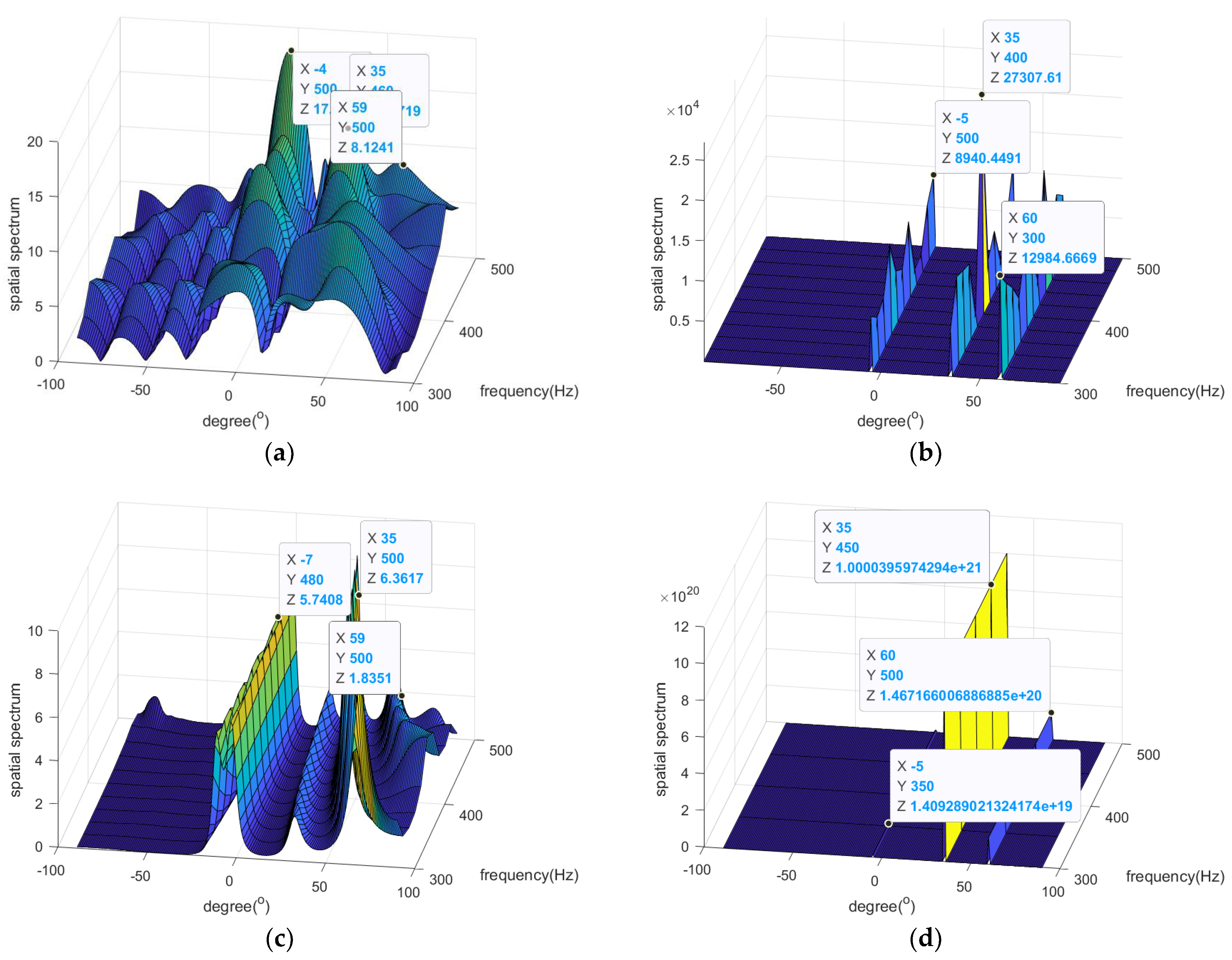
Experiment 1 tests angular resolution of various algorithms. Other conditions: DOA set { 5 , 35 , 60 } (ensure on grid), S N R = 20 d B , number of snapshots T = 20 . As shown in Figure 2, the estimated values of proposed method and ISSM are most precise. Note that proposed method possesses smoother peak values, which expresses small fluctuation with respect to frequency and proves better joint sparsity performance of proposed
Method than ISSM. The results can be explained by the fact that SBL is able to convergence at sparse solutions and possesses robustness to ordinary condition change itself, and proposed method has the ability to enhance sparsity more and stabilize the estimated values of DOA between different frequencies. In a word, proposed method remains the advantages of sparse Bayesian learning and shows better estimation performance than ordinary methods based on SBL.
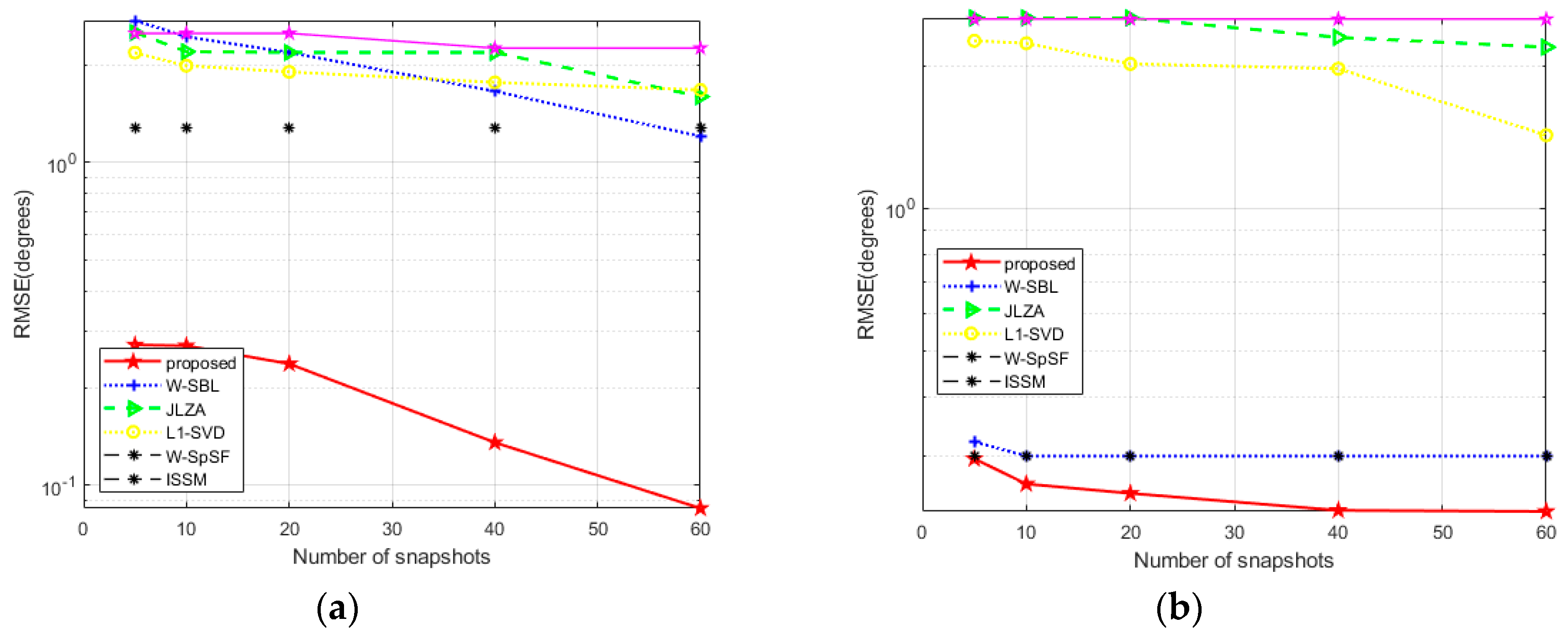
Experiment 2 examines estimation precision of various algorithms. Other conditions: DOA set { 5.5 , 35.1 , 60.2 } (ensure off grid). In Figure 3 and Figure 4, four conclusions can be drawn (1) the RMSE performance of proposed method is most excellent; (2) proposed method depend less on number of snapshots than others; (3) the estimation performance of proposed method improves most with SNR increasing; (4) proposed method achieves perfect estimation performance.

5. Conclusions

In this paper, we further expand the use and performance of sparse Bayesian learning with respect to wideband signal by transforming MMV model into block-sparse model. The main contributions are as below: the hierarchical Bayesian prior framework is constructed to favour sparsity; the corresponding iterative process is derived and completed; the whole method is proposed and applied to solve underdetermined DOA estimation problems. In some way, our proposed mehtod fully succeeds the advantages of sparse Bayesian learning and gains more excellent estimation performance and sparse recovery ability. Simulation results of two experiments are presented to prove the superior of our method, such as favouring sparsity, joint sparsity, high estimation accuracy, stable estimated values and strong adaptability.

References

  1. Krim, H.; Viberg, M. Two decades of array signal processing research: the parametric approach. IEEE SIGNAL PROC MAG 1996, 13, 67–94. [Google Scholar] [CrossRef]
  2. Liu, C.; Zakharov, Y.V.; Chen, T. Broadband underwater localization of multiple sources using basis pursuit de-noising. IEEE T SIGNAL PROCES 2011, 60, 1708–1717. [Google Scholar] [CrossRef]
  3. Liu, Z.M.; Huang, Z.T.; Zhou, Y.Y. An efficient maximum likelihood method for direction-of-arrival estimation via sparse Bayesian learning. IEEE T WIREL COMMUN 2012, 11, 1–11. [Google Scholar] [CrossRef]
  4. Su, G.; Morf, M. The signal subspace approach for multiple wide-band emitter location. IEEE T WIREL COMMUN 1983, 31, 1502–1522. [Google Scholar]
  5. Allam, M.; Moghaddamjoo, A. Two-dimensional DFT projection for wideband direction-of-arrival estimation. IEEE T SIGNAL PROCES 1995, 43, 1728–1732. [Google Scholar] [CrossRef]
  6. Wang, H.; Kaveh, M. Coherent signal-subspace processing for the detection and estimation of angles of arrival of multiple wide-band sources. IEEE Trans. Acoust, Speech, Signal Processing 1985, 33, 823–831. [Google Scholar] [CrossRef]
  7. Hung, H.; Kaveh, M. Focussing matrices for coherent signal-subspace processing. IEEE Trans. Acoust, Speech, Signal Processing 1988, 36, 1272–1281. [Google Scholar] [CrossRef]
  8. El-Keyi, A.; Kirubarajan, T. Adaptive beamspace focusing for direction of arrival estimation of wideband signals. SIGNAL PROCESS 2008, 88, 2063–2077. [Google Scholar] [CrossRef]
  9. Tang, Z.; Blacquiere, G.; Leus, G. Aliasing-free wideband beamforming using sparse signal representation. IEEE T SIGNAL PROCES 2011, 59, 3464–3469. [Google Scholar] [CrossRef]
  10. Shen, Q.; Liu, W.; Cui, W.; et al. Underdetermined DOA estimation under the compressive sensing framework: A review. IEEE ACCESS 2016, 4, 8865–8878. [Google Scholar] [CrossRef]
  11. Gan, L.; Wang, X. DOA estimation of wideband signals based on slice-sparse representation. EURASIP J ADV SIG PR 2013, 2013, 1–10. [Google Scholar] [CrossRef]
  12. Qin, Y.; Liu, Y.; Liu, J.; et al. Underdetermined wideband DOA estimation for off-grid sources with coprime array using sparse Bayesian learning. SENSORS-BASEL 2018, 18, 253. [Google Scholar] [CrossRef] [PubMed]
  13. Hyder, M.M.; Mahata, K. Direction-of-Arrival Estimation Using a Mixed l2,0.Norm Approximation. Norm Approximation. IEEE T SIGNAL PROCES 2010, 58, 4646–4655. [Google Scholar] [CrossRef]
  14. Malioutov, D.; Cetin, M.; Willsky, A.S. A sparse signal reconstruction perspective for source localization with sensor arrays. IEEE T SIGNAL PROCES 2005, 53, 3010–3022. [Google Scholar] [CrossRef]
  15. He, Z.Q.; Shi, Z.P.; Huang, L.; et al. Underdetermined DOA estimation for wideband signals using robust sparse covariance fitting. IEEE SIGNAL PROC LET 2014, 22, 435–439. [Google Scholar] [CrossRef]
  16. Hu, N.; Sun, B.; Zhang, Y.; et al. Underdetermined DOA estimation method for wideband signals using joint nonnegative sparse Bayesian learning. IEEE SIGNAL PROC LET 2017, 24, 535–539. [Google Scholar] [CrossRef]
  17. Zhao, L.; Li, X.; Wang, L.; et al. Computationally efficient wide-band DOA estimation methods based on sparse Bayesian framework. IEEE T VEH TECHNOL 2017, 66, 11108–11121. [Google Scholar] [CrossRef]
  18. Wipf, D.P.; Rao, B.D. Sparse Bayesian learning for basis selection. IEEE T SIGNAL PROCES 2004, 52, 2153–2164. [Google Scholar] [CrossRef]
  19. Wipf, D.P.; Rao, B.D. An empirical Bayesian strategy for solving the simultaneous sparse approximation problem. IEEE T SIGNAL PROCES 2007, 55, 3704–3716. [Google Scholar] [CrossRef]
  20. Zhang, Z.; Rao, B.D. Sparse signal recovery with temporally correlated source vectors using sparse Bayesian learning. IEEE J-STSP 2011, 5, 912–926. [Google Scholar] [CrossRef]
  21. Tzikas, D.G.; Likas, A.C.; Galatsanos, N.P. The variational approximation for Bayesian inference. IEEE SIGNAL PROC MAG 2008, 25, 131–146. [Google Scholar] [CrossRef]
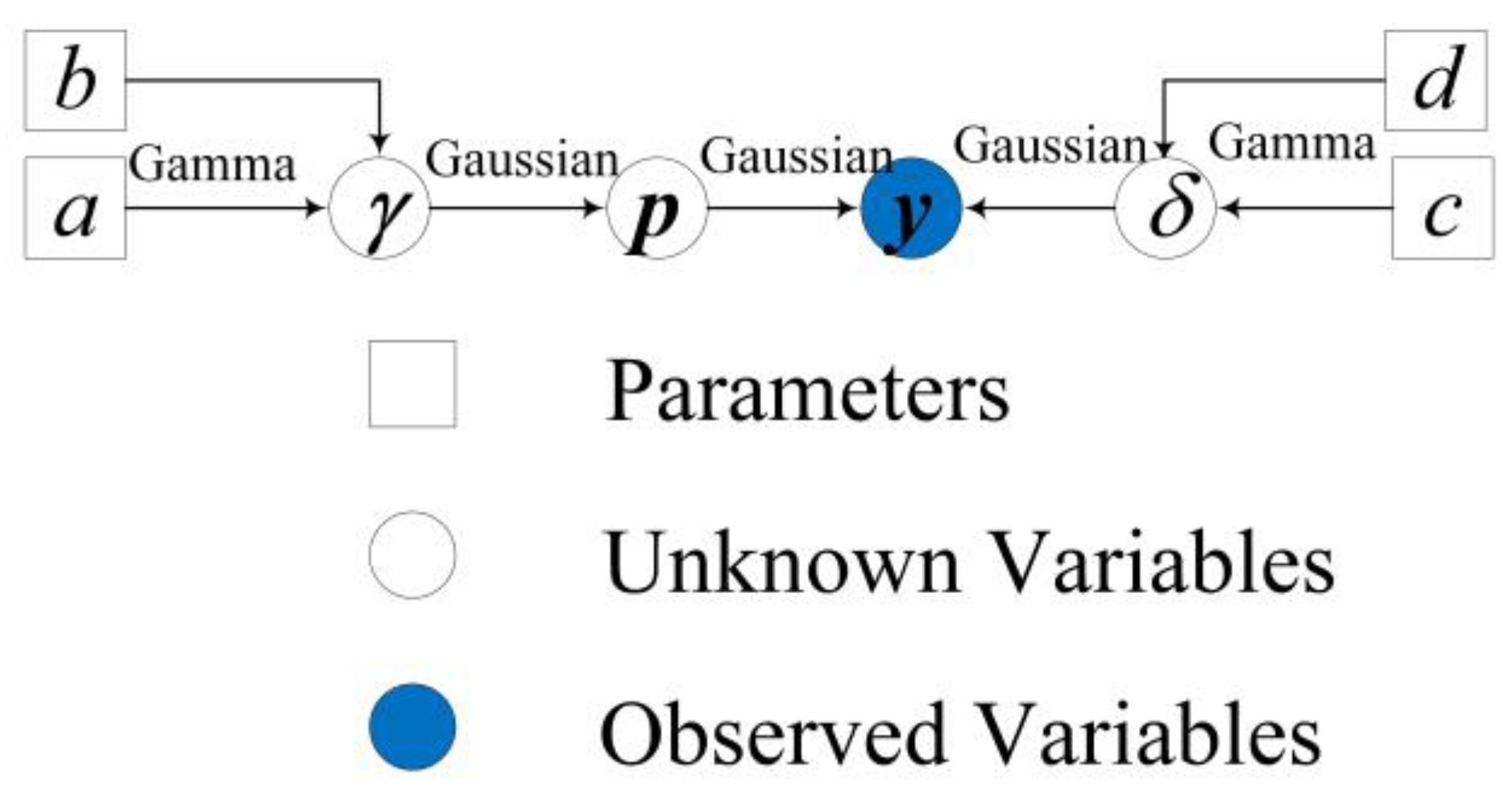
Figure 1. Directed acyclic graph of proposed Bayesian model.
Preprints 73519 g001
Figure 2. Spatial spectrum versus degree and frequency: (a) JLZA, (b) ISSM, (c) l 1 -SVD, (d)proposed method.
Preprints 73519 g002
Figure 3. RMSE versus SNR, (a) T = 5 , (b) T = 20 .
Preprints 73519 g003
Figure 4. RMSE versus number of snapshots, (a) S N R = 10 d B , (b) S N R = 20 d B .
Preprints 73519 g004
Disclaimer/Publisher’s Note: The statements, opinions and data contained in all publications are solely those of the individual author(s) and contributor(s) and not of MDPI and/or the editor(s). MDPI and/or the editor(s) disclaim responsibility for any injury to people or property resulting from any ideas, methods, instructions or products referred to in the content.
Copyright: This open access article is published under a Creative Commons CC BY 4.0 license, which permit the free download, distribution, and reuse, provided that the author and preprint are cited in any reuse.
Prerpints.org logo

Preprints.org is a free preprint server supported by MDPI in Basel, Switzerland.

Subscribe

© 2024 MDPI (Basel, Switzerland) unless otherwise stated