Impact of Cooperation and Intra-Specific Competition of Prey on the Stability of Prey-Predator Models with Refuge

Preprint

Article

Impact of Cooperation and Intra-Specific Competition of Prey on the Stability of Prey-Predator Models with Refuge

Altmetrics

Downloads

163

Views

Comments

A peer-reviewed article of this preprint also exists.

This version is not peer-reviewed

Submitted:

29 May 2023

Posted:

31 May 2023

You are already at the latest version

Alerts

Abstract

The main objective of this study is to find out the influence of cooperation and intra-specific competition in escaping predation through refuge of the prey population and the effect of the two intra-specific interactions on the dynamics of prey-predator systems. For this purposes, two mathematical models with Holling type-II functional response function have been proposed and analyzed. The first model includes cooperation among prey populations whereas the second one incorporates intra-specific competition. Existence conditions and stability of different equilibrium points of both models have been carried out for the qualitative behaviour of the systems. Refuge through intra-specific competition has a stabilizing role, whereas cooperation has a destabilizing role on the system dynamics. Periodic oscillations are observed in both the systems through Hopf bifurcation. From the analytical and numerical findings, we conclude that intra-specific competition affects the prey population and continuously checks the refuge class under a critical value, and thus it never becomes too large to cause predator extinction due to food scarcity. Conversely, cooperation leads maximum individuals to escape predation through the refuge so that predators will suffer from low predation success.

Keywords:

Subject: Computer Science and Mathematics - Applied Mathematics

1. Introduction

Prey-predator interaction has immense importance in the existence of life. In predator-prey systems, the prey population shows a variety of defense to escape from predation [1,2]. Among them, the refuge is most common in literature [3,4], and it has become a significant issue in theoretical ecology [5]. One famous proverb about the Fox-Rabbit chase says: “The fox is only running for his dinner, but the rabbit is running for his life [6]”. If the rabbit can successfully save its life, it’s called the rabbit refuge of the fox. So, the refuge can be defined as any strategy that decreases the rate of predation [7].

Refuge can be done in two ways– (i) constant numerical refuge, where an definite number of individuals in the population refuge predation, and (ii) proportional refuge, where a fixed proportion of individuals in the population refuge predation. In both cases, the whole prey population can’t attain the facility of refuge, and thus, a particular number or fraction of the population is always exposed to the predator. If not, the predator population will no longer be able to persist, and the system will be destabilized.

If we consider a situation where a constant number of safe refuge places is available and thus only a definite number of individuals in the population can enjoy the facility of refuge. In such condition, two habitats are available for the prey population– either lives in the refuge or roam around in the open habitat where they are available to predator [22]. In [23], authors considered a prey-predator model with constant numerical prey refuge and showed that, there are two major factors that control this type of refuge in the population: (i) population density of prey (x) and available refuge (m). When

x \leq m

, competition among prey for refuge is negligible since prey fitness depends only on predation [22]. In such condition cooperation among individuals of the prey population must be seen. But this is not the case for all time because this type of refuge can include a definite number of individuals and thus they cannot move freely between habitats when population size exceeds refuge number (

x > m

) and obviously intra-specific competition to take refuge will increase proportionally as density increases. The conclusion regarding this type of refuge is that it has a strong stabilizing effect [24] it can prevent the extinction of prey, but when the population is too large to stay all in the refuge then coexistence with predators is expected as the predator will get continuous resources [22]. So, in that case, mortality rate of the prey increases when population density goes beyond the refuge capacity and this will cause a negative feedback stabilizing effect to the system [25].

Another situation is where a proportion of individuals in the population refuge the predation. In such condition, there are also two habitats available for the prey population– either lives in the refuge or roam around in the open habitat where they are available to predator [22]. But in that case a continuous movement of prey individuals occur between open habitat and refuge [26]. In [27], Kar proposed the Lotka-Volterra type prey-predator system including proportional prey refuge where, m is denoted as the fractional refuge of prey for predator and it ranges from

0 < m < 1

. Now, if we consider the whole prey population as x then

m x

portion of the prey is in refuge habitat, and

(1 - m) x

of the prey is in open habitat and thus available to the predator. In case of proportional refuge, the whole population never get the opportunity to attain refuge and thus, the process of finding refuge place is either cooperation or competition based. This type of refuge can reduce mortality rate of prey by reducing predation pressure and can effect positively the growth of prey and negatively that of predator. Thus, in this way refuge can act as a stabilizing effect in prey-predator dynamics [32]. On other extreme refuge may destabilize prey-predator dynamics as the predator population become extinct by suffering from lower predation success due to large refuge size [33].

Mathematically prey-predator interaction was first described by Alfred James Lotka in 1925 [8] and Vito Volterra in 1927 [9]. Georgy Frantsevich Gause in 1934 [10] first found refuge in his experiment with protozoan predator Didinium feeding on Paramecium. One major drawback of the Lotka-Volterra model was that the predator never becomes saturated. Crawford Stanley Holling solved this problem [11,12,13] by suggesting three kinds of functional responses (Holling type I, II, and III) for different species of predator. Rosenzweig and MacArthur in 1963 [14] first replaced the linear functional response of Lotka–Volterra model with the Holling type-II response function and first documented that prey-predator coexistence is not limited to a stable equilibrium; a limit cycle appears when the stable equilibrium undergoes the Hopf bifurcation [15]. Hassel in 1978 [20] showed that adding a large number of refuges to a model in which the absence of a refuge exhibits divergent oscillation replaces the oscillatory behavior with a stable equilibrium. Since then, various modeling approaches for the prey-predator system, including refuge, have been done by researchers [16,17,18,19,27,28].

In the previous articles ([28,29,31] and the references therein), authors have considered competition among predator populations. In our knowledge, this article is the first article to consider the impact of cooperation and intra-specific competition within the prey population for attaining refuge. The key question of this study is– “how does the prey-predator system dynamics being impacted when the decision of refuge is made through cooperation and same for the intra-specific competition?” To get an answer to this problem, we have developed two mathematical models. The first model includes the cooperation among prey populations, whereas the second model contains the intra-specific competition. The dynamics of the models have been analyzed with qualitative theories.

This paper has been carried out sequentially in the latter sections as follows. Section 2 deals with the mathematical model formation with prey refuge and cooperation and local stability and Hopf bifurcation also shown. Another mathematical model with prey refuge and intra-specific competition is formed and the existence of Hopf bifurcation and stability analysis is done in Section 3. Global stability of co-existing equilibrium are analyzed in Section 4. Section 5 deals with findings of direction of Hopf bifurcation. Numerical simulation results are delineated in Section 6. The final discussion and biological interpretation of the results of the present study are included in the concluding (Section 7).

2. Mathematical Model for Prey Refuge and Cooperation

Here, we propose the Lotka-Volterra type prey-predator system including proportional prey refuge and cooperation making the following assumptions:

There are two populations in the model namely

x (t)

is the prey population size,

y (t)

is the population size of the predator at any time t. r is the intrinsic growth rate, and k is the carrying capacity of the prey,

γ

is the death rate of the predator in the absence of prey,

β

is the predation rate, and c is the conversion factor denoting the efficiency of predators for each captured prey.

Also,

\frac{β}{a}

is the maximum number of prey that the predator per unit time can eat;

\frac{1}{a}

being the half-saturation constant.

The term

\frac{β x}{1 + a x}

denotes the predator’s response to prey. This type of predator response function is known as Holling type-II functional response.

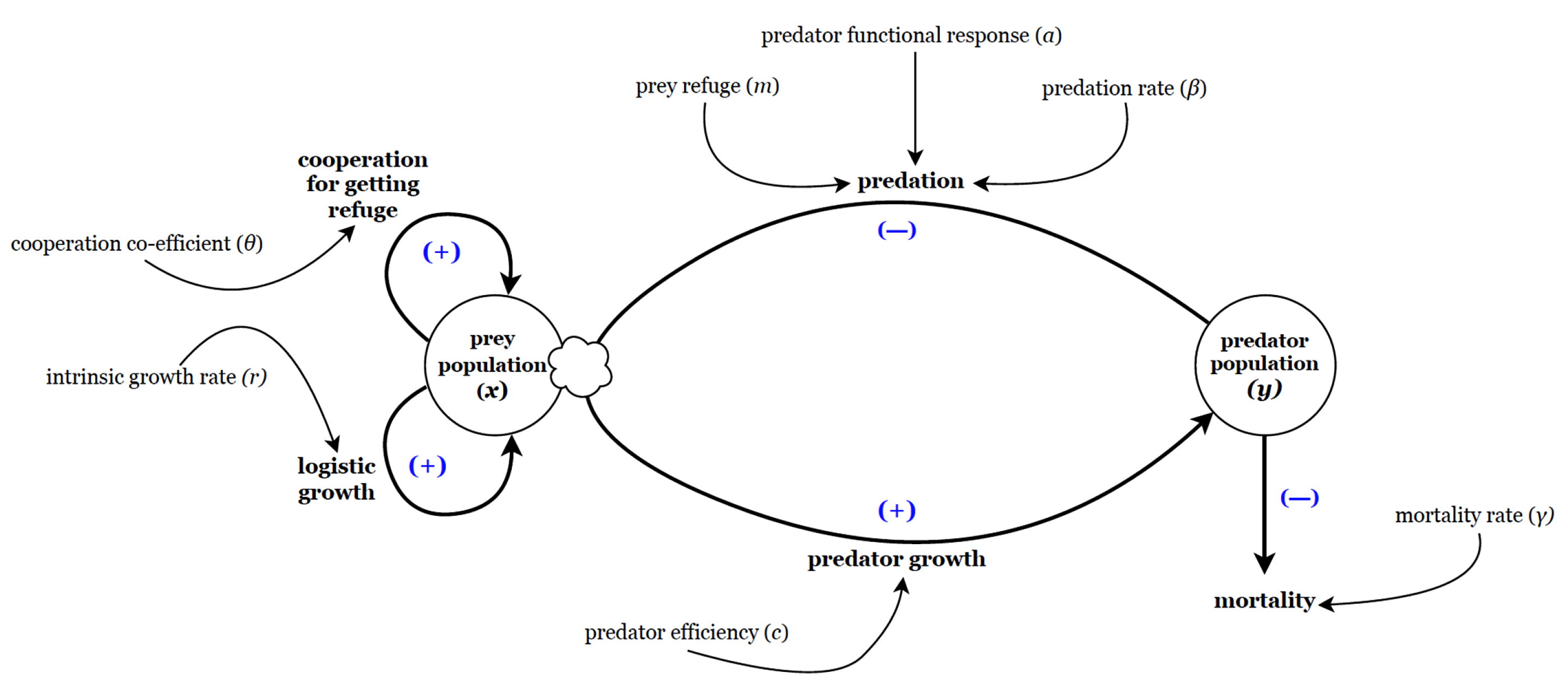
Let m be the fractional refuge of prey for predator,

0 < m < 1

and constant. So,

m x (t)

portion of the prey is in refuge habitat and

(1 - m) x (t)

of the prey is in open habitat and thus available to the predator, and

θ

is the cooperation co-efficient among prey population trying to escape predation pressure through refuge.

Using the assumptions discussed above, we get the following mathematical model:

\begin{matrix} \frac{d x}{d t} & = & r x [1 - \frac{x}{k}] - \frac{β (1 - m) x y}{1 + a (1 - m) x} + θ x^{2}, \\ \frac{d y}{d t} & = & - γ y + \frac{c β (1 - m) x y}{1 + a (1 - m) x}, \end{matrix}

(1)

with the initial biological condition

x (0) > 0, y (0) > 0

(2)

It is assumed that all the system parameters are positive constants. The schematic diagram of the model (1) is shown in Figure 1.

In the next subsection, we determine all the possible equilibrium points and existence conditions for their biological feasibility of the model (1).

2.1. Boundedness of Solutions

Biologically, all population of the model should be finite. For this boundedness analysis is significant. We have derived the following theorem for boundedness of the solutions of the model (1).

Theorem 1.

All solutions of the model (1) with the given initial conditions (2) are nonnegative and bounded for all time

t > 0

Proof.

We rewrite the first equation of (1),

\begin{matrix} \frac{d x}{d t} & = & r x [1 - \frac{x}{k}] - \frac{β (1 - m) x y}{1 + a (1 - m) x} + θ x^{2} = x h (x, y), \end{matrix}

(3)

where,

h (x, y) = r [1 - \frac{x}{k}] - \frac{β (1 - m) y}{1 + a (1 - m) x} + θ x

. Therefore

\begin{matrix} \frac{d x}{x} & = & h (x, y) d t \\ x (t) & = & x (0) exp \{\int_{0}^{t} h (x, y) d t\} \end{matrix}

Since

x (0) > 0

, we can conclude that

x (t)

is always positive. Similarly, the nonnegativity of

y (t)

can be established.

For boundedness analysis, we define

W = x + y

. Now, adding the two equations of (1), we can obtain

\begin{matrix} \frac{d W}{d t} & = & r x [1 - \frac{x}{k}] - \frac{β (1 - m) x y}{1 + a (1 - m) x} + θ x^{2} - γ y + \frac{c β (1 - m) x y}{1 + a (1 - m) x}, \end{matrix}

As by definition,

c \leq 1

. Using this fact, we can write

\begin{matrix} \frac{d W}{d t} & \leq & r x [1 - \frac{x}{k}] + θ x^{2} - γ y \\ = & r x [1 - \frac{x}{k}] + θ x^{2} - γ (x + y) + γ x . \end{matrix}

(4)

Now,

g (x) = r x [1 - \frac{x}{k}] + θ x^{2} + γ x

is a function of x only. It has a maximum value at

x = \frac{k (r + γ)}{2 (r - k θ)}

and the maximum value is

M_{θ} = \frac{k {(r + γ)}^{2}}{4 (r - k θ)}

. Thus, from (4), we get

\begin{matrix} \frac{d W}{d t} & \leq & M_{θ} - γ W \end{matrix}

Using the theory of functional differential equation, we have

lim sup_{t \to \infty} W = \frac{M_{θ}}{γ} .

(5)

□

The set

D

defined by

D = {(x, y) \in R_{+}^{2} : 0 \leq x + y \leq M_{θ},}

(6)

where

M_{θ} = \frac{k {(r + γ)}^{2}}{4 (r - k θ)}

, is positively invariant and each solution that starts in

D

remains in

D

2.2. Existence of Equilibria

In this subsection, we analyze the existence and stability of positive solution of the system (1).

Model (1) has three equilibrium points viz (i) the trivial equilibrium

{\bar{E}}_{0} (0, 0)

, (ii) the predator-free equilibrium

{\bar{E}}_{1} (\frac{r k}{r - θ k}, 0)

, and (iii) the coexisting equilibrium

{\bar{E}}^{*} ({\bar{x}}^{*}, {\bar{y}}^{*})

, where

\begin{matrix} {\bar{x}}^{*} = \frac{γ}{(1 - m) (c β - a γ)}, \\ {\bar{y}}^{*} = \frac{1}{β (1 - m)} {1 + a (1 - m) {\bar{x}}^{*}} [θ {\bar{x}}^{*} + \frac{r (k - {\bar{x}}^{*})}{k}] . \end{matrix}

(7)

Now

y^{*}

is positive if

θ {\bar{x}}^{*} + \frac{r (k - {\bar{x}}^{*})}{k} > 0

which after simple calculations gives

{\bar{x}}^{*} > \frac{r k}{r - θ k}

Using the fact that

0 < m < 1

and from above discussion, we have the following result for the existence of the equilibria of the system (1).

Proposition 1.

(i): Predator-free equilibrium of the system (1) is feasible if $θ < \frac{r}{k}$ , and
(ii): the coexisting equilibrium ${\bar{E}}^{*}$ is feasible if $\frac{c β}{a} > γ$ and ${\bar{x}}^{*} > \frac{r k}{r - θ k}$ .

Remark 1.

When the cooperation for attaining refuge (θ) is less than the overall intra-specific competition on logistic growth of prey (

\frac{r}{k}

), the predator-free equilibrium

{\bar{E}}_{1}

of the system (1) is feasible, otherwise it will not exist. On the other hand, when the utilization efficiency of predator after successful predation (

\frac{c β}{a}

) is greater than the mortality rate of predator in absence of prey (γ), then the coexisting equilibrium

{\bar{E}}^{*}

will exist.

2.3. Stability Analysis and Hopf Bifurcation

Here, we examine the stability of each biological feasible equilibrium. We perturb the ODE system nearby any equilibrium point

\bar{E} (x, y)

, and get the system

\frac{d X}{d t} = J X,

where

X = {[x, y]}^{T}

and J is the Jacobian matrix.

The Jacobian J for the system (1) is:

J = [J_{i j}] = [\begin{matrix} r x (1 - \frac{2 x}{k}) - \frac{β (1 - m) y}{{(1 + a (1 - m) x)}^{2}} + 2 θ x & - \frac{β (1 - m) x}{1 + a (1 - m) x} \\ \frac{c β (1 - m) y}{{(1 + a (1 - m) x)}^{2}} & - γ + \frac{c β (1 - m) x}{(1 + a (1 - m) x)} \end{matrix}] .

Characteristic equation of the Jacobian matrix is given by

f (ξ) = ξ^{2} + l_{1} ξ + l_{2} = 0 .

(8)

An equilibrium point

E (x, y)

is stable if both the roots of (8) is negative or having negative real parts. The conditions for this is

l_{1} > 0 a n d l_{2} > 0,

(9)

where

l_{1} = - (J_{11} + J_{22}), l_{2} = J_{11} J_{22} - J_{21} J_{12} .

The equilibrium

E (x, y)

is unstable if any of the above conditions are violated.

Hopf bifurcation will occur if both the roots of (8) are purely imaginary for a particular value of the model parameter (called bifurcation parameter). Suppose

η

a bifurcation parameter, then for bifurcation to occur, the following condition must be satisfied:

\begin{matrix} (i) & l_{1} = 0, l_{2} > 0, \\ (i i) & \frac{\partial l_{1}}{\partial η} \neq 0 . \end{matrix}

(10)

Condition (i) will give the critical value of the bifurcation parameter and condition (ii) is the transversality condition.

The Jacobian matrix J at the trivial equilibrium

{\bar{E}}_{0} (0, 0)

has a positive eigenvalue r, thus it is always unstable.

At the predator-free equilibrium

{\bar{E}}_{1} (\bar{x_{1}}, 0)

, the Jacobian matrix is

J ({\bar{E}}_{1}) = [\begin{matrix} r \bar{x_{1}} (1 - \frac{2 \bar{x_{1}}}{k}) + 2 θ \bar{x_{1}} & - \frac{β (1 - m) \bar{x_{1}}}{1 + a (1 - m) \bar{x_{1}}} \\ 0 & - γ + \frac{c β (1 - m) \bar{x_{1}}}{(1 + a (1 - m) \bar{x_{1}})} \end{matrix}],

where

\bar{x_{1}} = \frac{r k}{r - θ k}

{\bar{E}}_{1}

is feasible when

\frac{r}{k} > θ

. Jacobian matrix has eigenvalues

ξ_{1} = r \bar{x} (1 - \frac{2 \bar{x}}{k}) + 2 θ \bar{x}

which is negative for

\frac{r}{k} > θ

, directly follows from the feasibility of

{\bar{E}}_{1}

. Another eigenvalue is

ξ_{2} = - γ + \frac{c β (1 - m) \bar{x}}{(1 + a (1 - m) \bar{x})}

which is negative if

θ > \frac{r γ - r k [c β (1 - m) - a (1 - m) γ]}{γ k}

The characteristic equation at the coexisting equilibrium

{\bar{E}}^{*}

ξ^{2} + {\bar{l}}_{1}^{*} ξ + {\bar{l}}_{2}^{*} = 0,

(11)

where

{\bar{l}}_{1}^{*} = - r {\bar{x}}^{*} (1 - \frac{2 {\bar{x}}^{*}}{k}) + \frac{β (1 - m) {\bar{y}}^{*}}{{(1 + a (1 - m) {\bar{x}}^{*})}^{2}} - 2 θ {\bar{x}}^{*},

{\bar{l}}_{2}^{*} = \frac{c β^{2} {(1 - m)}^{2} {\bar{x}}^{*} {\bar{y}}^{*}}{{(1 + a (1 - m) {\bar{x}}^{*})}^{3}} > 0 .

The eigenvalues are negative or having negative real parts if

{\bar{l}}_{1}^{*} > 0

{\bar{l}}_{2}^{*} > 0

holds always.

From the above discussion we have the following theorem for the stability of the three equilibrium of system (1).

Theorem 2.

(i): The trivial equilibrium ${\bar{E}}_{0} (0, 0)$ is always unstable.
(ii): ${\bar{E}}_{1}$ is feasible if $\frac{r}{k} > θ$ and is stable if $θ < \frac{r γ - r k (1 - m) [c β - a γ]}{γ k}$ , consequently transcritical bifurcation occurs if $θ = \frac{r γ - r k (1 - m) [c β - a γ]}{γ k}$ .
(iii): ${\bar{E}}^{*}$ is stable if ${\bar{l}}_{1}^{*} > 0$ and unstable for ${\bar{l}}_{1}^{*} < 0$ . Hopf bifurcation occurs if ${\bar{l}}_{1}^{*} = 0$ and $\frac{\partial l_{1}^{*}}{\partial θ} |_{θ = θ^{*}} \neq 0$ , where $θ^{*}$ is the critical value of the bifurcation parameter θ.

3. The Mathematical Model for Prey Refuge and Intra-specific Competition

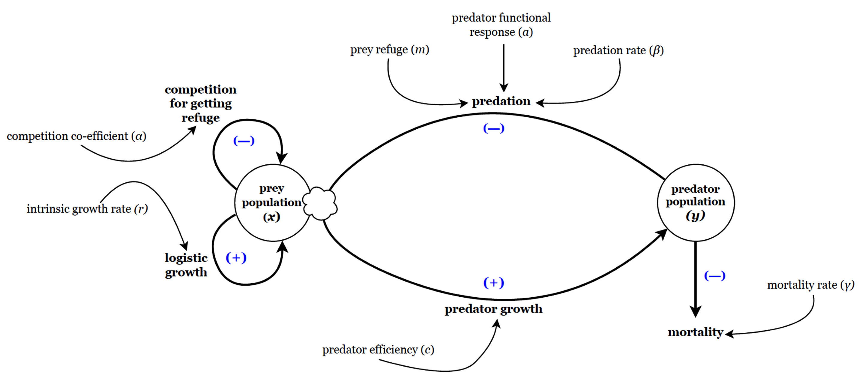
The flow chart of this situation is given in Figure 2. From this we propose the Lotka-Volterra type prey-predator system including proportional prey refuge and competition as follows:

\begin{matrix} \frac{d x}{d t} & = & r x [1 - \frac{x}{k}] - \frac{β (1 - m) x y}{1 + a (1 - m) x} - α x^{2}, \\ \frac{d y}{d t} & = & - γ y + \frac{c β (1 - m) x y}{1 + a (1 - m) x} . \end{matrix}

(12)

Where,

α

is the competition co-efficient among prey population trying to escape predation pressure through refuge and all other parameters are already defined in the previous model (1).

Remark 2.

From the mathematical point of view, model (1) and model (12) is differ only in one term

- α x^{2}

in place of

θ x^{2}

. Thus in the analytical results (dynamics) of model (12) can be derived from the analysis of model (1).

From the analysis of the previous section (using Theorem 1) we have derived the following theorem.

3.1. Boundedness of Solutions

Theorem 3.

Each solution of model (12) with positive initial conditions remains nonnegative and bounded in

S

for all time

t > 0

, where,

S = {(x, y) \in R_{+}^{2} : 0 \leq x + y \leq M_{α},}

(13)

where

M_{α} = \frac{k {(r + γ)}^{2}}{4 (r + k α)} .

3.2. Existence of Equilibria

The model (12) has three equilibrium points viz (i) the trivial equilibrium

{\tilde{E}}_{0} (0, 0)

, (ii) predator free equilibrium

{\tilde{E}}_{1} (\frac{r k}{r + α k}, 0)

, and (iii) the coexisting equilibrium

{\tilde{E}}^{*} ({\tilde{x}}^{*}, {\tilde{y}}^{*})

, where

\begin{matrix} {\tilde{x}}^{*} & = & \frac{γ}{(1 - m) (c β - a γ)}, \end{matrix}

(14)

\begin{matrix} {\tilde{y}}^{*} & = & \frac{1}{β (1 - m)} {1 + a (1 - m) {\tilde{x}}^{*}} [- α {\tilde{x}}^{*} + \frac{r (k - {\tilde{x}}^{*})}{k}] . \end{matrix}

(15)

In model (12),

{\tilde{E}}_{1}

always exists and

{\tilde{E}}^{*}

exists for

\frac{c β}{a} > γ

and

- α {\tilde{x}}^{*} + \frac{r (k - {\tilde{x}}^{*})}{k} > 0

. Last condition gives

{\tilde{x}}^{*} < \frac{r k}{k α + r}

. Thus we have the following result.

Proposition 2.

(i): Predator-free equilibrium of the system (12) always exists.
(ii): The coexisting equilibrium ${\tilde{E}}^{*}$ is feasible if $\frac{c β}{a} > γ$ and ${\tilde{x}}^{*} < \frac{r k}{r + α k}$ .

Remark 3.

In model (1), existence of predator-free equilibrium

{\bar{E}}_{1}

depends on θ but in model (12) the equilibrium always exists. One major explanation behind this may be cooperation for attaining refuge (θ) may cause behavioral contradiction among the prey population as they compete in almost all aspects except finding refuge, and for that reason, θ becomes a critical factor for the existence of equilibrium.

3.3. Stability and Hopf Bifurcation

The Jacobian is at any steady point

\tilde{E} (x, y)

of system (12) is given below:

J (E) = [J_{i j}] = [\begin{matrix} r x (1 - \frac{2 x}{k}) - \frac{β y}{{(1 + a x)}^{2}} - 2 α x & - \frac{β x}{1 + a x} \\ \frac{c β y}{{(1 + a x)}^{2}} & - γ + \frac{c β x}{(1 + a x)} \end{matrix}] .

Using the stability analysis of the previous section (using Theorem 2, we can establish the following theorem for the stability of the equilibrium points of the system (12).

Theorem 4.

(i): The trivial equilibrium ${\tilde{E}}_{0} (0, 0)$ is always unstable.
(ii): ${\tilde{E}}_{1}$ is stable if $α < \frac{r k (1 - m) [c β - a γ] - r γ}{γ k}$ , and unstable for $α > \frac{r k (1 - m) [c β - a γ] - r γ}{γ k}$ consequently transcritical bifurcation occurs at $α = \frac{r k (1 - m) [c β - a γ] - r γ}{γ k}$ .
(iii): ${\tilde{E}}^{*}$ is stable if ${\tilde{l}}_{1}^{*} > 0$ and unstable for ${\tilde{l}}_{1}^{*} < 0$ . Hopf bifurcation occurs if ${\tilde{l}}_{1}^{*} = 0$ and $\frac{\partial {\tilde{l}}_{1}^{*}}{\partial α} |_{α = α^{*}} \neq 0$ , where $α^{*}$ denotes the critical value of the bifurcation parameter α. In this case,

${\tilde{l}}_{1}^{*} = - r {\tilde{x}}^{*} (1 - \frac{2 {\tilde{x}}^{*}}{k}) + \frac{β (1 - m) {\tilde{y}}^{*}}{{(1 + a (1 - m) {\tilde{x}}^{*})}^{2}} + 2 α {\tilde{x}}^{*},$

and

${\tilde{l}}_{2}^{*} = \frac{c β^{2} {(1 - m)}^{2} {\tilde{x}}^{*} {\tilde{y}}^{*}}{{(1 + a (1 - m) {\tilde{x}}^{*})}^{3}} > 0 .$

4. Global Stability of $E^{*}$

The following theorem establish the global stability of the interior equilibrium

E^{*}

Theorem 5.

The interior equilibrium

E^{*}

is globally asymptotically stable if the condition mentioned below are satisfied:

\begin{matrix} (i) & k θ < r, \\ (i i) & \frac{r k}{θ k - r} < x^{*} < \frac{γ}{β} . \end{matrix}

(16)

Proof.

We construct the suitable Lyapunov function V as,

V = (x - x^{*} - x^{*} ln \frac{x}{x^{*}}) + (y - y^{*} - y^{*} ln \frac{y}{y^{*}}) .

(17)

It is easy to verify that V is positive definite for all

(x, y) \in R_{+}^{2} ∖ (x^{*}, y^{*})

. Now we take the derivative of V along the solutions of the system (1) and obtain the following,

\begin{matrix} \frac{d V}{d t} & = & (x - x^{*}) \frac{\dot{x}}{x} + (y - y^{*}) \frac{\dot{y}}{y}, \\ = & (x - x^{*}) [r [1 - \frac{x}{k}] - \frac{β (1 - m) y}{1 + a (1 - m) x} + θ x] + (y - y^{*}) [- γ + \frac{c β (1 - m) x}{1 + a (1 - m) x}] . \end{matrix}

Rearranging the equation (18) we get, following,

\begin{matrix} \frac{d V}{d t} & = & x^{2} (- \frac{r}{k} + θ) + x (r + \frac{r x^{*}}{k} - θ x^{*}) - r x^{*} + (\frac{c β x y}{1 + a x} - \frac{β x y}{1 + a x}) + (\frac{β x^{*} y}{1 + a x} - γ y) \\ - \frac{c β x y^{*}}{1 + a x} - γ y^{*} - γ y + y (\frac{β x^{*}}{1 + a x} - γ) . \end{matrix}

Thus, if the conditions given in (16) holds, then the right hand side of (18) is negative definite. Thus

\frac{d V}{d t} < 0

, along all the trajectories in the first quadrant except

(x^{*}, y^{*})

. Also we have

\frac{d V}{d t} |_{E^{*}} = 0

. The proof follows from the suitable Lyapunov function V and Lyapunov-LaSalle’s invariant principle (cf. Hale [39]). Hence, the interior equilibrium point

E^{*}

is globally asymptotically stable if the condition (16) is satisfied. □

5. Direction of Hopf Bifurcation

In this section, we analyse the stability nature and direction of the Hopf bifurcating periodic solutions. For this, we consider the transformation,

u_{1} = x - x_{*}

u_{2} = y - y_{*}

, which transform the system (1) to the following system,

\begin{matrix} {\dot{u}}_{1} & = & a_{1} u_{1} + a_{2} u_{2} + \underset{i, j \geq 0}{\sum_{i + j = 2}} a_{i j} u_{1}^{i} u_{2}^{j} + \underset{i, j \geq 0}{\sum_{i + j = 2}} a_{i j} u_{1}^{i} u_{2}^{j} + \dots \end{matrix}

(18)

\begin{matrix} {\dot{u}}_{2} & = & b_{1} u_{1} + b_{2} u_{2} + \underset{i, j \geq 0}{\sum_{i + j = 2}} b_{i j} u_{1}^{i} u_{2}^{j} + \underset{i, j \geq 0}{\sum_{i + j = 2}} b_{i j} u_{1}^{i} u_{2}^{j} + \dots, \end{matrix}

(19)

where

a_{i j}

and

b_{i j}

, are determined by using the following relations,

\begin{matrix} a_{i j} = \frac{1}{i! j!} \frac{\partial^{i + j} (F_{1})}{\partial x^{i} \partial y^{j}}, b_{i j} = \frac{1}{i! j!} \frac{\partial^{i + j} (F_{2})}{\partial y^{i} \partial y^{j}} . \end{matrix}

(20)

where,

a_{1} = \frac{\partial F_{1}}{\partial x}

a_{2} = \frac{\partial F_{2}}{\partial y}

, etc., and

\begin{matrix} F_{1} = r x [1 - \frac{x}{k}] - \frac{β (1 - m) x y}{1 + a (1 - m) x} - α x^{2}, \\ F_{2} = - γ y + \frac{c β (1 - m) x y}{1 + a (1 - m) x} . \end{matrix}

We get the following relations from Hassard et al. [21],

\begin{matrix} [\begin{matrix} u_{1} \\ u_{2} \end{matrix}] = z q + \bar{z} \bar{q} + W, \end{matrix}

(21)

where

\begin{matrix} z (t) = 〈 q^{*}, u_{t} 〉, W (t, θ) = u_{t} (θ) - 2 Re {z (t) q (θ)} . \end{matrix}

(22)

Thus,

\begin{matrix} \dot{z} & = & i ω_{0} z + {\bar{v}}_{1} f_{0}^{1} + {\bar{v}}_{2} f_{0}^{2} + {\bar{v}}_{3} f_{0}^{3} \\ = & i ω_{0} z + \frac{1}{2} g_{20} z^{2} + g_{11} z \bar{z} + \frac{1}{2} g_{02} {\bar{z}}^{2} + \frac{1}{6} g_{30} z^{3} + \frac{1}{6} g_{03} {\bar{z}}^{3} + \frac{1}{2} g_{21} z^{2} \bar{z} + \frac{1}{2} g_{12} z {\bar{z}}^{2} \\ + & O (| z |^{4}), \end{matrix}

(23)

We calculate the values of

g_{20}

g_{02}

g_{11}

and

g_{21}

by comparing the coefficients of

z^{2}

{\bar{z}}^{2}

z \bar{z}

and

z^{2} \bar{z}

. Hence

\begin{matrix} C_{1} (0) & = & \frac{i}{2 ω_{0}} (g_{11} g_{20} - 2 {| g_{11} |}^{2} - \frac{| g_{02} |^{2}}{3}) + \frac{g_{21}}{2}, \end{matrix}

(24a)

\begin{matrix} μ_{2} & = & - \frac{Re (C_{1} (0))}{Re (η^{'} (0))}, \end{matrix}

(24b)

\begin{matrix} β_{2} & = & 2 Re (C_{1} (0)), \end{matrix}

(24c)

\begin{matrix} τ_{2} & = & - \frac{Im (C_{1} (0)) + μ_{2} Im (η^{'} (0))}{ω_{0}}, \end{matrix}

(24d)

where,

\begin{matrix} Im (η^{'} (0)) = \frac{d (Im (η (α)))}{d α} ∣_{α = α^{*}} = [\frac{σ_{1}}{\sqrt{σ_{2}}} \frac{\dot{σ_{3}} - (\dot{σ_{1}} σ_{2} + σ_{1} \dot{σ_{2}})}{2 (σ_{1}^{2} + σ_{2})} + \frac{(σ_{1} + σ_{2}) {\dot{σ}}_{2}}{2 \sqrt{σ_{2}} (σ_{1}^{2} + σ_{2})}] ∣_{α = α^{*}} . \end{matrix}

The stability and direction can be determined from the following theorem [28,38].

Theorem 6.

The nature of the bifurcating periodic solutions from the values of

β_{2}, μ_{2}

and

τ_{2}

in the center manifold at the threshold value

α^{*}

(i) If

μ_{2}

is positive (negative), then the system (1) emits a stable (unstable) limit cycle for

α > α^{*}

(

α < α^{*}

(ii)

β_{2}

determines the stability of the bifurcating periodic solutions: the bifurcating periodic solutions are stable (unstable) if

β_{2} < 0

(β_{2} > 0)

and

(iii)

τ_{2}

determines the period of periodic solutions: the period increases (decreases) if

τ_{2} > 0

(τ_{2} < 0)

A similar theorem can be obtained for the parameter

θ

from Theorem 6.

6. Numerical Simulations

In this section, we provide numerical examples for visualizing the dynamical regimes that can be seen in our model systems analysed in the previous sections. Parameter values with detailed descriptions and units used for the simulation are given in Table 1. The value of carrying capacity is taken as

k = 4

assuming that the maximum number of 4 prey can be supported within a

3 m \times 3 m

square area. Though conversion efficiency (c) varies within a range of

0 - 1

, we have considered

c = 0.75

for the simulations. The results obtained from simulations are discussed in the following subsections.

6.1. Numerical Simulation of System (1)

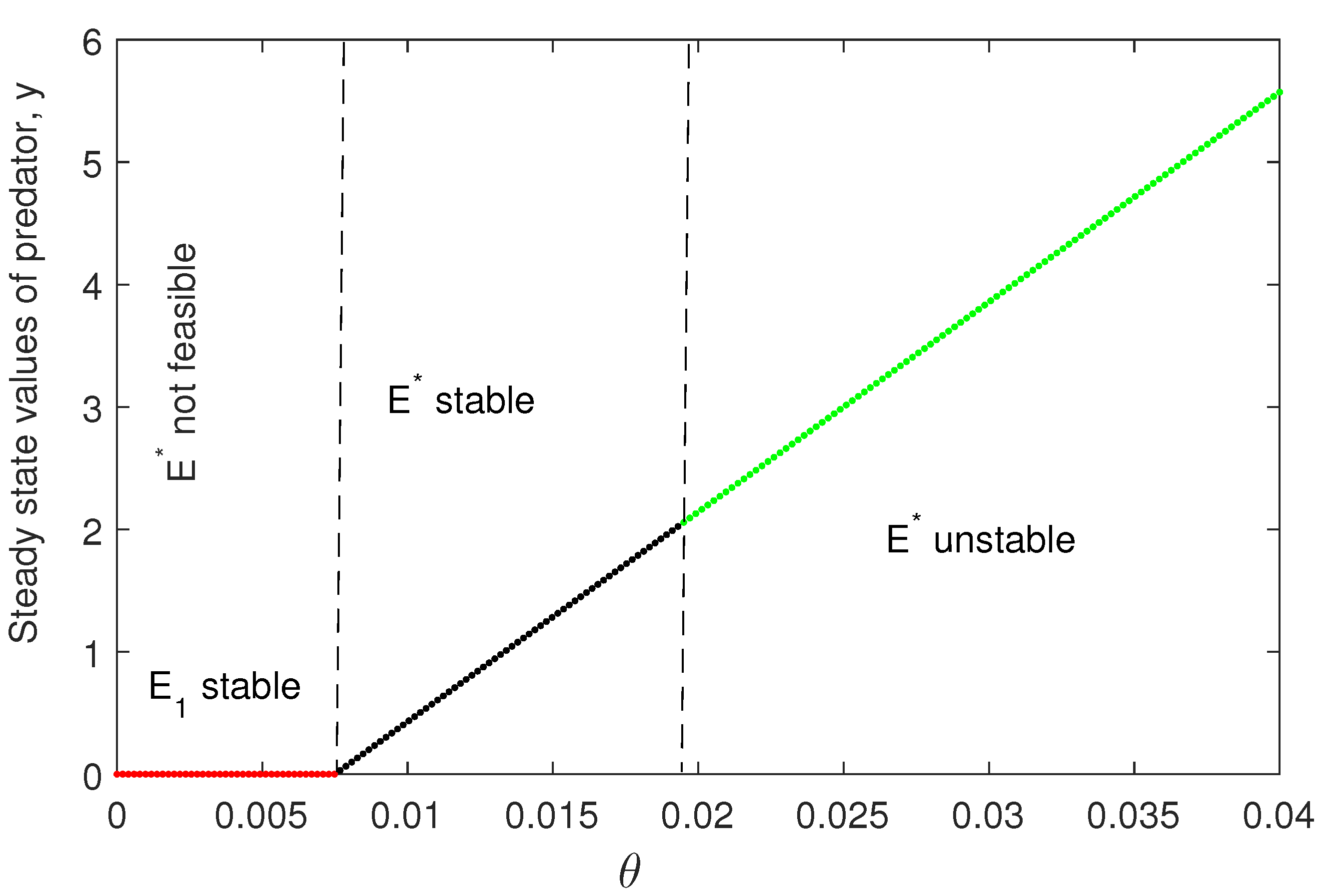
Here, simulation of system (1) is discussed. In Figure 3, we have plotted the transcritical forward bifurcation of

{\bar{E}}_{1}

and existence of

{\bar{E}}^{*}

by varying parameter

θ

. For some large value of theta,

{\bar{E}}^{*}

becomes unstable (Theorem 2).

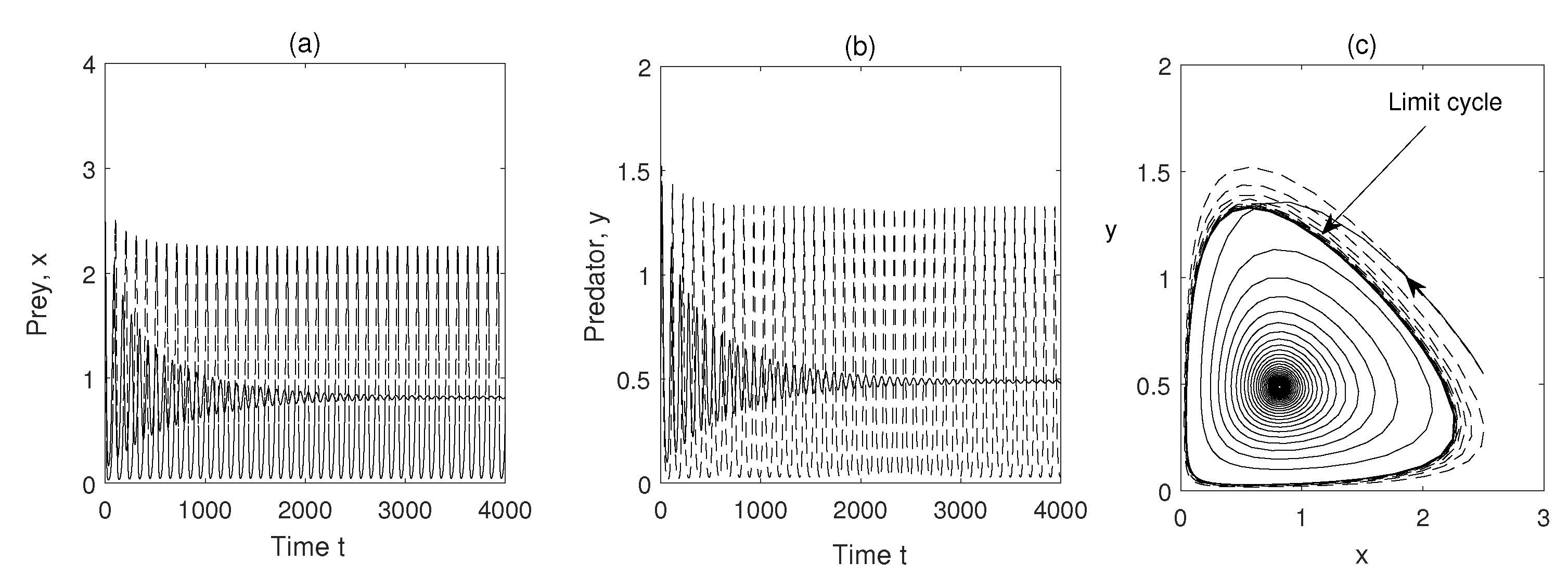
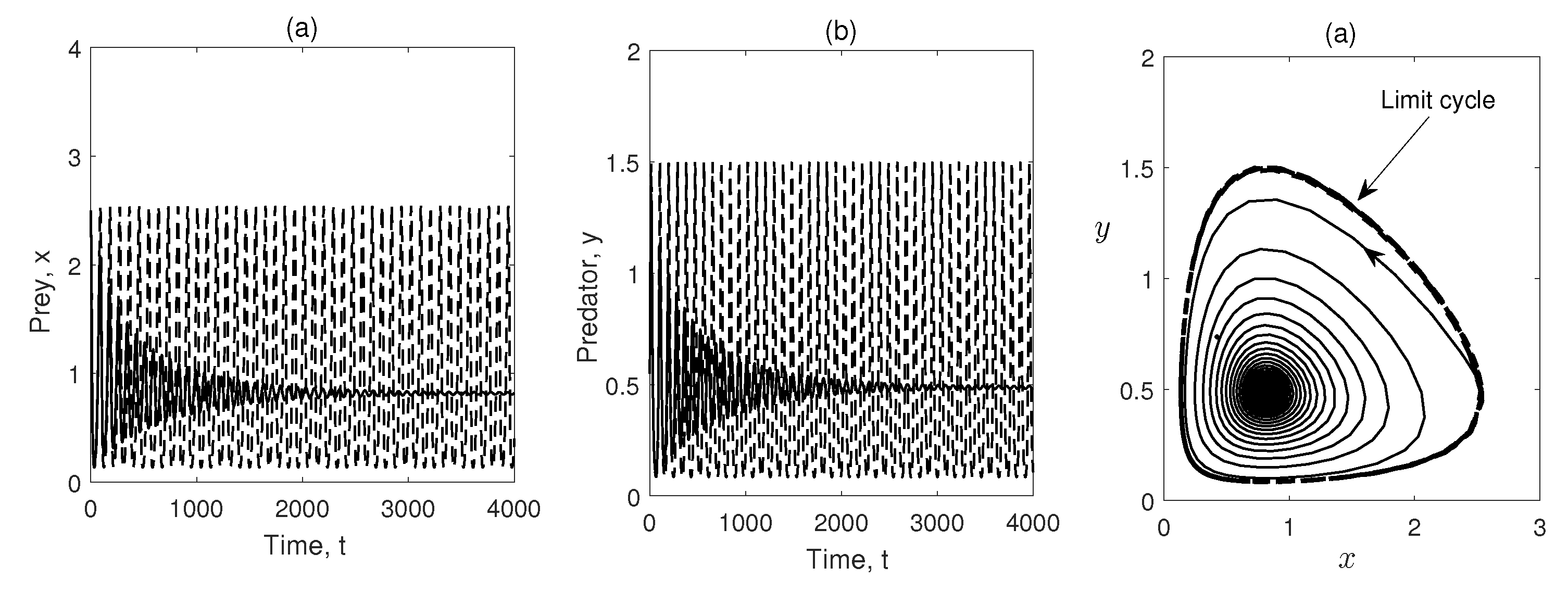
In Figure 4, we have seen limit cycle for

m = 0

, (other parameters are given in Table 1) i.e. limit cycle can occur if refuge is neglected. But if we take

m = 0.3

(i.e.,

30 %

of the total prey population are in refuge habitat and rest

70 %

are vulnerable to predation) the limit cycle disappears and coexisting equilibrium becomes a stable focus.

In Figure 5, we have taken

m = 0.3, θ = 0

(i.e., there is no cooperation among the prey population for finding refuge habitat) the system is stable. Then we increase the value of

θ

(i.e., increasing cooperation among the prey individuals for finding safe refuge place) and seen limit cycle for

θ = 0.005

(other parameters are given in Table 1). From this we can conclude that the impact of

θ

is destabilising the stable steady state.

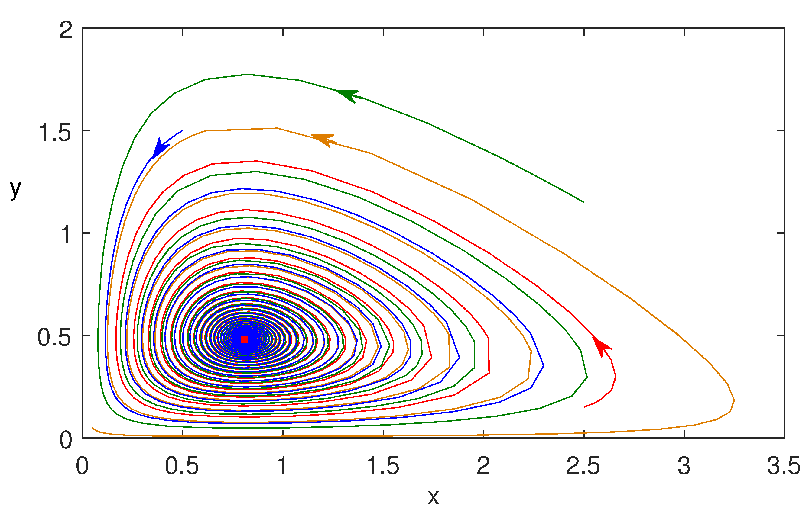
Figure 6 is plotted for three different initial values of the model variables. This shows the nonlinear stability of coexisting equilibrium

E^{*}

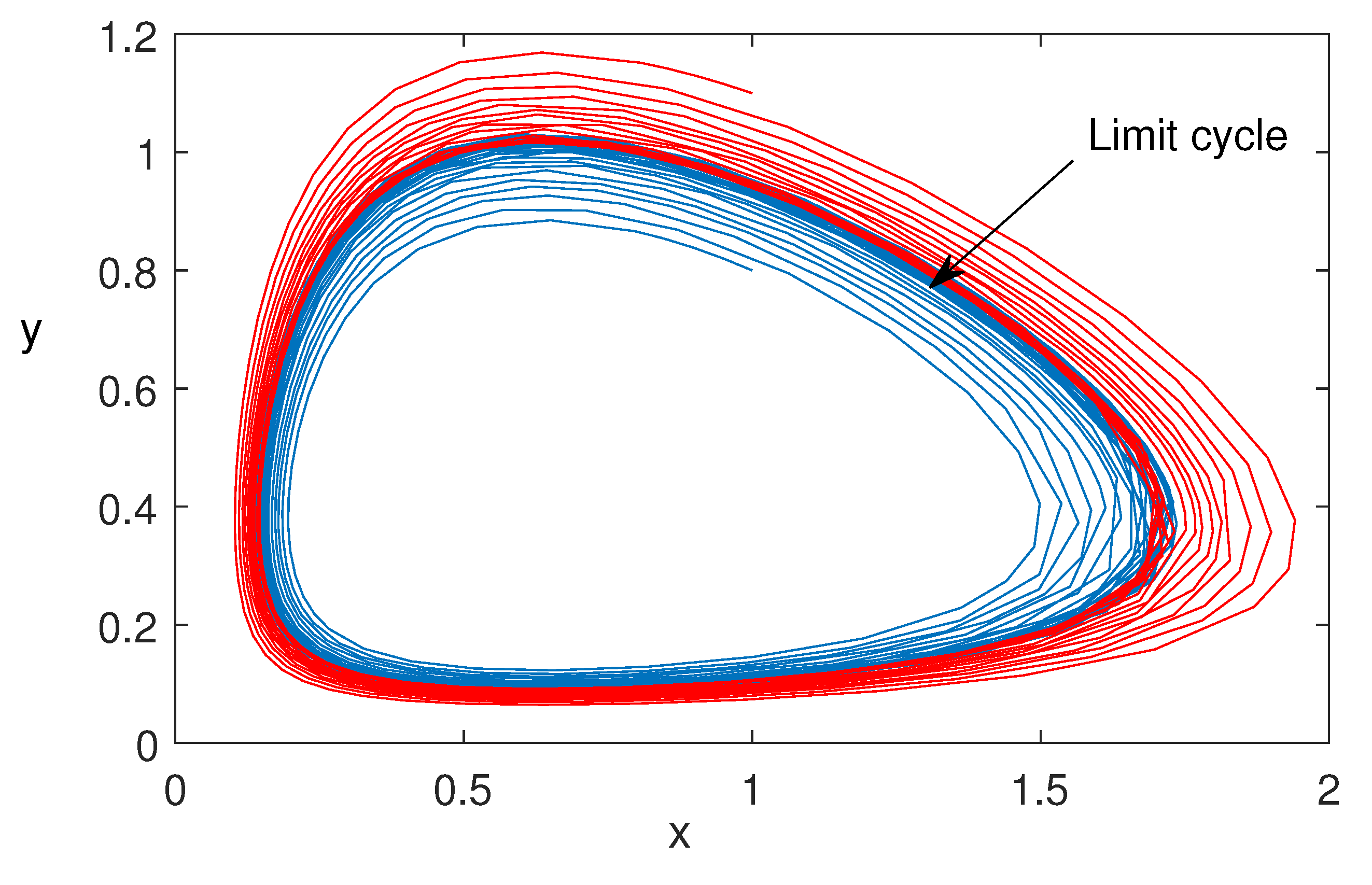
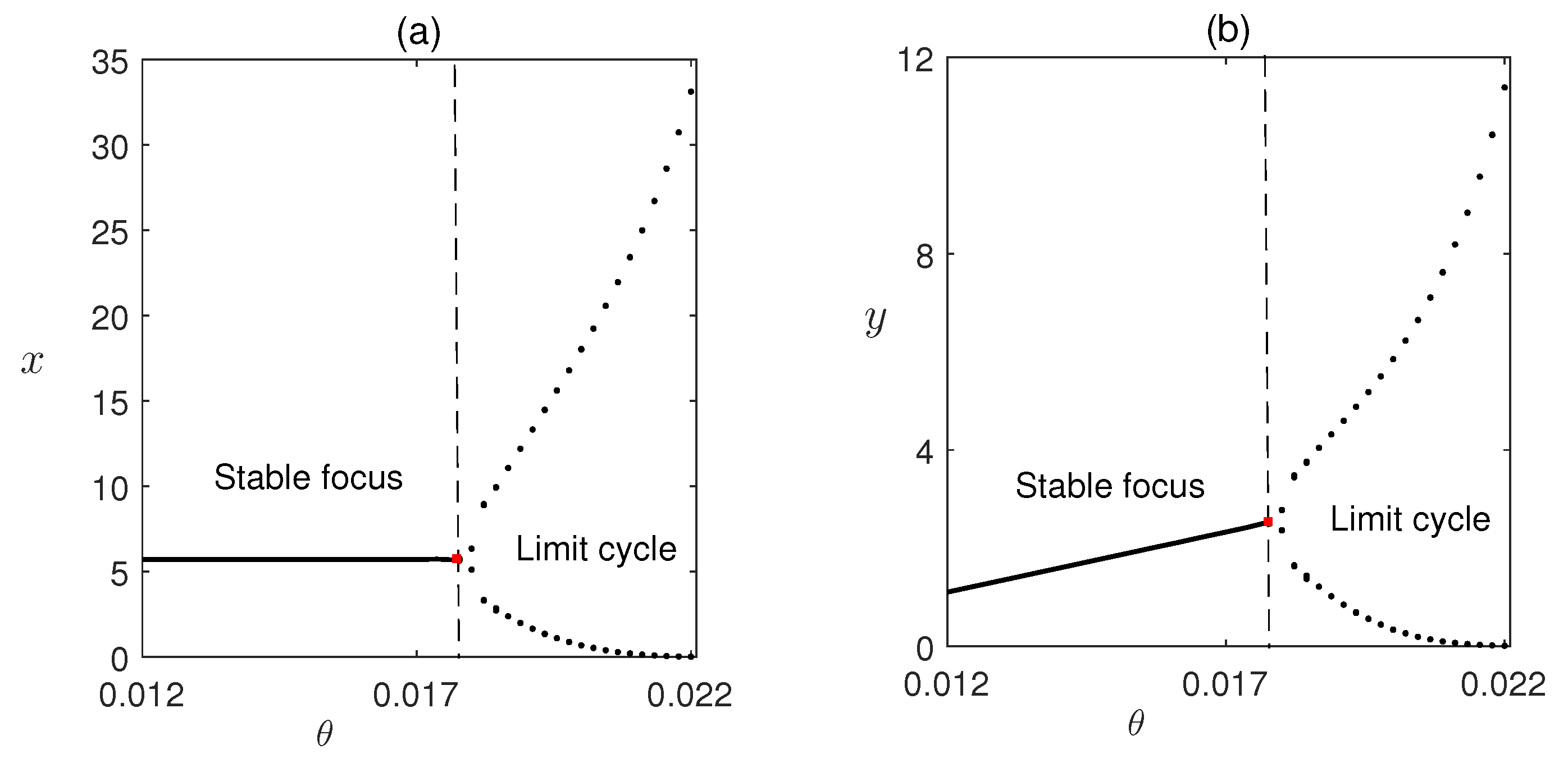
. Figure 7 is also plotted for two different initial values of the model variables. This figure shows that the bifurcating periodic solutions are stable and Hopf bifurcation is of supercritical type. In Figure 8, we have plotted the Hopf bifurcation diagram taking

θ

as the main parameter. Limit cycle appear as the parameter

θ

crosses the critical value (Theorem 2).

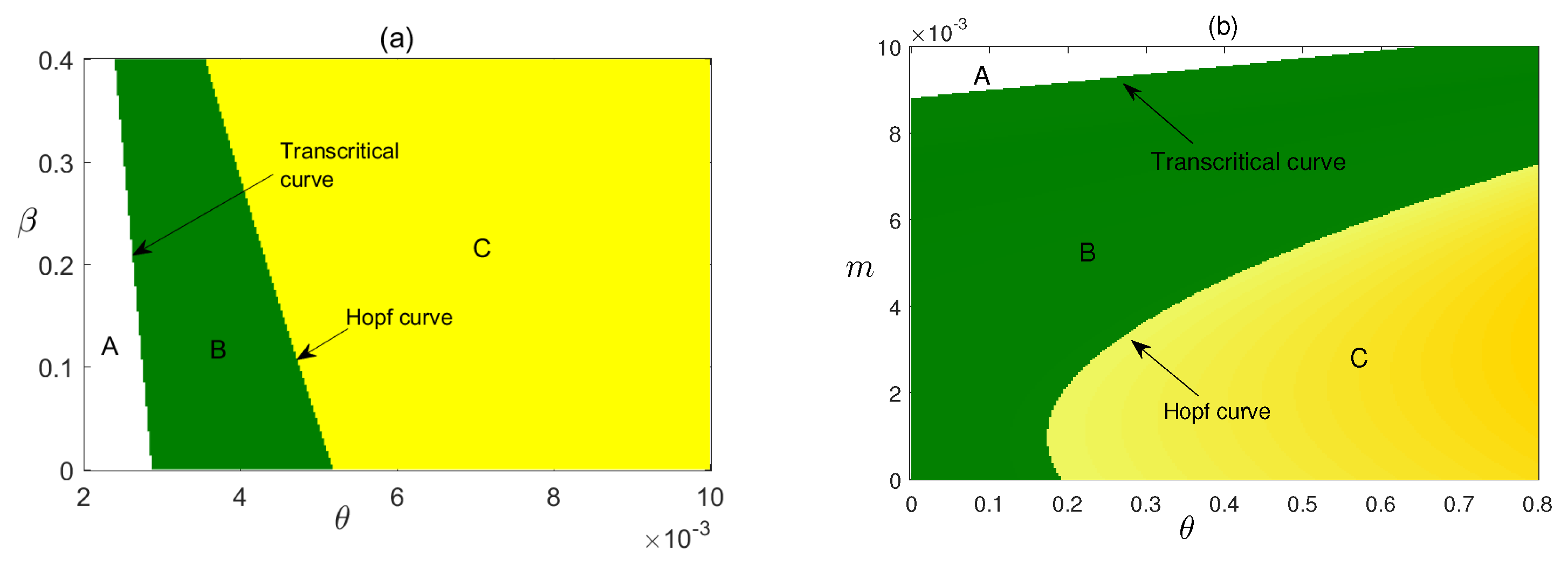
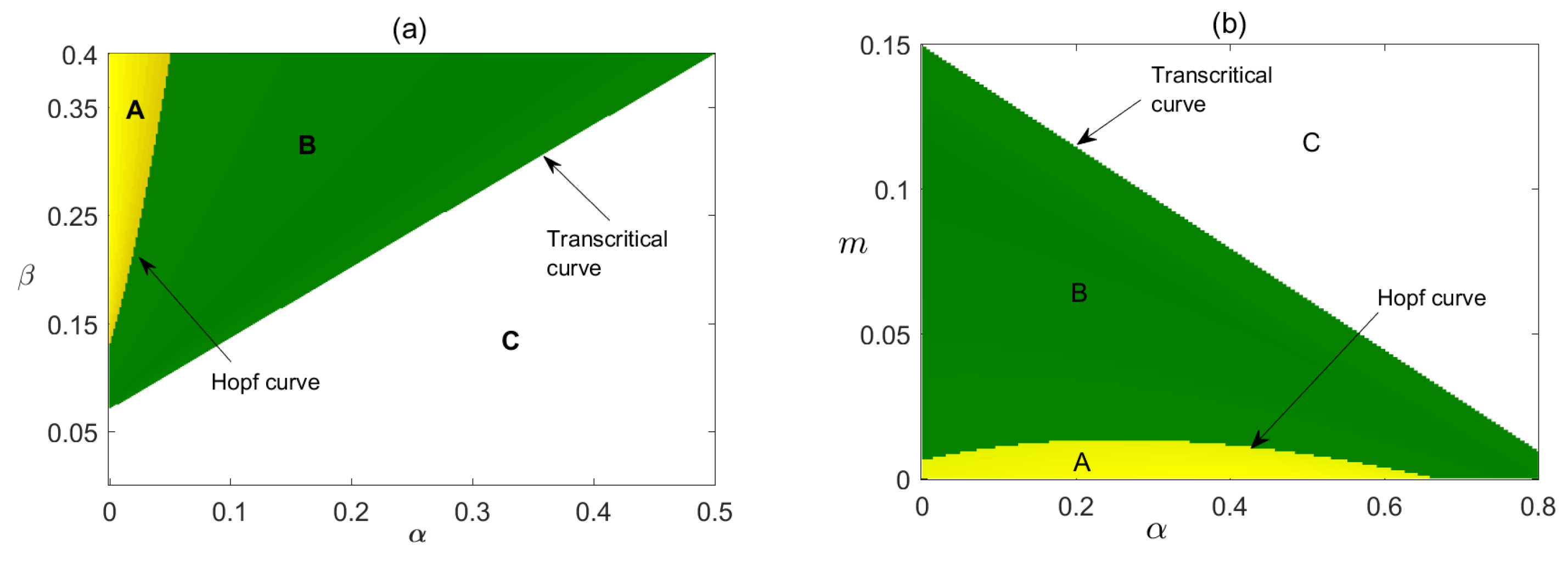
In Figure 9, we have plotted the stability regions of coexisting equilibrium in

θ - β

and

θ - m

parameter planes. In Figure 9a, it is shown how parameters

θ

and

β

critically affect the stability of the system. We have observed that for the very low value of

θ

{\bar{E}}^{*}

is not feasible but

{\bar{E}}_{1}

is stable and as

θ

crosses its critical value

{\bar{E}}^{*}

becomes stable and the stability of

{\bar{E}}^{*}

depends on the combined value of

θ

and

β

as higher values can make the stable system unstable via Hopf bifurcation. In Figure 9b direct relationship between parameter

θ

and m to the stability of the system has shown, where with the increased value of

θ

only a very high value of m can make the system stable.

From the simulations, we observe that

θ

is one of the critical parameters for the model system (1), stability of different equilibria depends on it. For very low value of

θ

{\bar{E}}^{*}

is not feasible but

{\bar{E}}_{1}

is stable and as

θ

crosses its critical value

{\bar{E}}^{*}

becomes stable via transcritical bifurcation and finally further higher values can make the

{\bar{E}}^{*}

unstable via Hopf bifurcation.

6.2. Numerical Simulation of System (12)

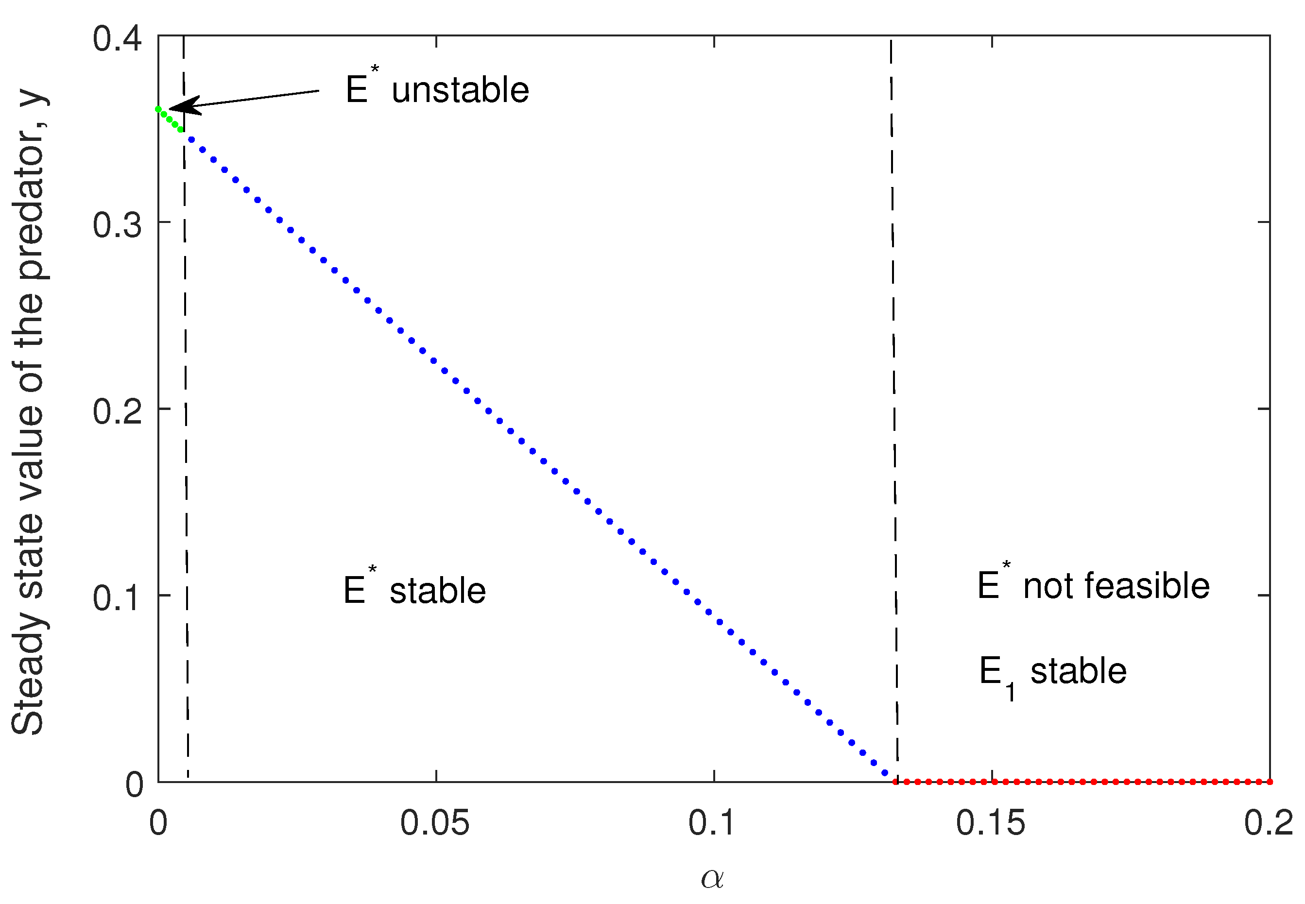
In Figure 10, we have plotted the transcritical forward bifurcation of

{\tilde{E}}_{1}

and existence of

{\tilde{E}}^{*}

varying the parameter

α

(Theorem 4).

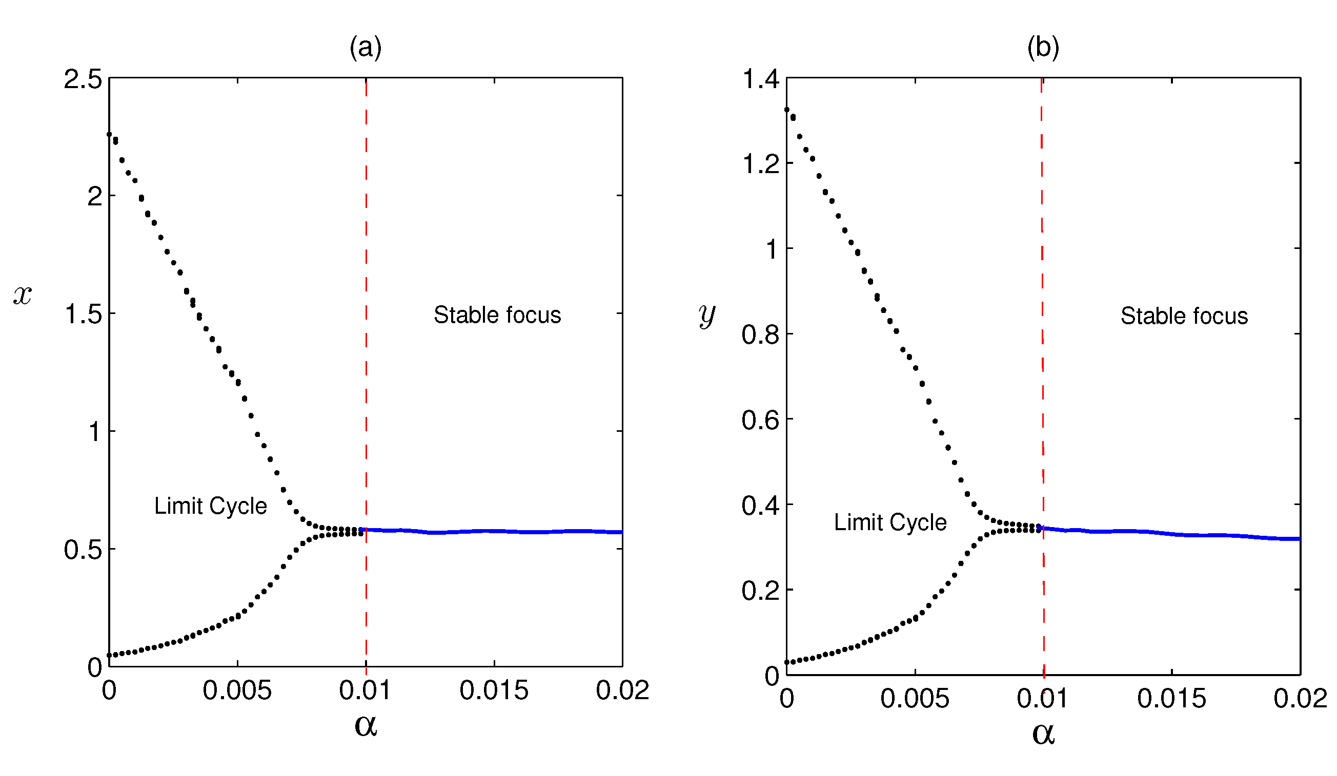
Hopf bifurcation diagram is plotted in Figure 11 taking

α

as the main parameter. The Limit cycle disappears as the parameter

α

crosses the critical value

α^{*}

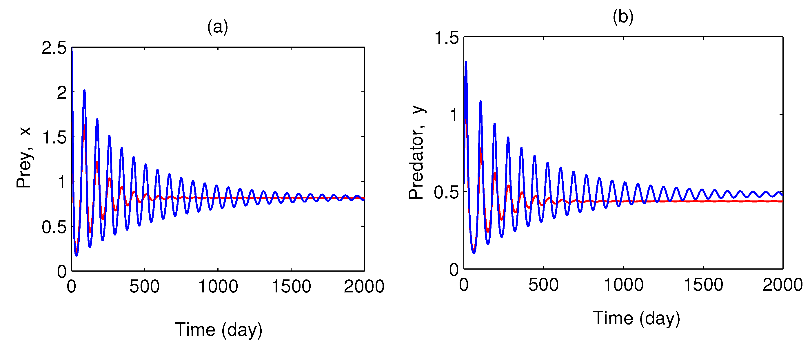
In Figure 12, we have taken

m = 0.3

α = 0.001

(i.e. there is very less competition among the prey individuals for finding refuge habitat) the system is stable. Now, if we increase the value of

α

to 0.01 (i.e., the prey individuals become ten times more competitive in the process of finding a safe refuge place), the system stabilizes faster (other parameters are given in Table 1). From this, we can conclude that

α

has stabilizing effect on the system.

In Figure 13, we have plotted the stability regions of coexisting equilibrium in

α - β

and

α - m

parameter planes. The area of stability regions increased as both the value of m and

α

are increased. But

β

can make the stable system unstable via Hopf bifurcation. The critical value of

β

, i.e.,

β^{*}

depends on the other model parameters such as

α

. Here we have shown that the critical value of

β

significantly depends on

α

. In (b) we have taken higher value of

β

, then we vary

α

and m. We have observed that

{\tilde{E}}^{*}

changes its stability to become stable, then is not feasible for higher values of m and

α

, but

{\tilde{E}}_{1}

is stable there.

Thus from the numerical simulations, we observe that for the model system (12), the stability of different equilibria depends on the parameter

α

. Here, for very low value of

α

{\tilde{E}}^{*}

is unstable and it becomes stable as

α

crosses the critical value via Hopf bifurcation but for very high value of

α

{\tilde{E}}^{*}

is not feasible where

{\tilde{E}}_{1}

becomes stable via transcritical bifurcation.

7. Discussion and Conclusion

In Hoogly-Matla estuarine mangrove ecosystem, there are several islands and those are criss-crossed by numerous creeks which originate from the main rivers. These creeks have rich detritus loads which come from the adjacent mangrove litter. Therefore, these creeks support many detritivorous fishes and one of such was described by Sarwardi et al. [29]. In their study (Sarwardi et al., 2013) described one important detritivorous fish of these creeks, namely Liza parsia which lives in the creeks and its predator Otolithoides pama visits the creeks only during high tide for capturing food. The mangrove plants in this region are extended from the supra-littoral zone to the lower-littoral zone up to the creek bed. During high tide as the water level comes up the lower parts of the plants submerge under the water and the bushy part of the submerged mangrove plants creates shelter for Liza parsia to avoid its predator. So, this spatial refuge is possible due to enhanced environmental heterogeneity in this ecosystem. But there is not enough refuge habitats to support all the individuals of the prey population and if it’s the case then the refuge decision among the prey population is made either though cooperation or by competition and our study is focused to find out the impact of these two intra-specific interaction in the system dynamics.

Prey-predator system with prey refuge has been a sought-after topic among ecological and mathematical modelers for almost the last five decades. Previous studies have assured that refuge has a stabilizing effect on prey-predator dynamics. Several models are already established with various conditions and situations. Still, another finding was that if the refuge class or fraction becomes too large, the predator faces food scarcity. The system becomes destabilized due to the extinction of the predator. But in any natural system, all members of a prey population can’t avoid predation at any given time; thus, continuous decision pressure works among them. The refuge among the prey population can happen in two ways – cooperatively or competitively, and these two inevitable intra-specific interactions must affect prey-predator dynamics. This study finds the impact of cooperation and intra-specific competition among prey populations trying to escape predation through the refuge on the stability of prey-predator dynamics.

For the two situations mentioned above, in this paper, we have considered a prey-predator system incorporating a prey refuge and assumed that the predator response function is of Holling type II. Cooperation (model (1)) and intra-specific competition (model (12)) among the prey population for escaping predation pressure through refuge are incorporated into the system to find out the process (either cooperation or intra-specific competition) for leading the population towards better stabilization.

Firstly, the stabilizing effect of refuge on the system dynamics has been shown (Figure 4), and after the addition of refuge, the system dynamics settle from limit cycle behavior to a stable equilibrium. The refuge protects the prey population from predators, and it reduces predation pressure. Over-exploitation of prey population by predator turns the prey population into a divergent oscillation state. But this vulnerable state is transformed into a stable state with the help of the prey population’s refuge strategies. The stable state of the prey population also makes a stable predator population.

When the decision of refuge is made cooperatively among the prey population, the stable equilibrium again goes back to a limit cycle condition which clearly denotes that cooperation has a destabilizing effect on the system dynamics during refuge (Figure 5). From the prey’s point of view, if the refuge is attained cooperatively, then maximum individuals can escape predation easily, which must be favorable for them but on the other hand predator will suffer from low predation success, and in an extreme situation, they will be eliminated from the system if the system is linear as a predator has no alternative option to predate.

Our study shows that the system reaches faster in the equilibrium state when the refuge facility is achieved through intra-specific competition among the prey population (Figure 12). Refugees during intra-specific competition have a stabilizing effect on the system dynamics. As intra-specific competition has a negative impact on individuals of the prey population, the refuge class is constantly checked and never too large to cause prey scarcity for a predator. A controlled amount of the prey population will always escape predation through the refuge, which helps the prey population for better survival and the predator population will not go extinct in any situation as they never face a crisis for food. Due to this balanced interaction, the system dynamics reach equilibrium faster.

In reality, the decision-making process to escape predation pressure by refuge either through competition or cooperation within a prey population is complex and doesn’t follow any hard and fast rules. Cooperation or competition in various prey organisms depends on the spatial heterogeneity of their habitat as when the shelter place (refuge size) is large enough to protect all prey individuals, then only cooperation acts as the deciding factor, but any scarcity in protected habitat turns the cooperative behavior into a competitive one.

It is more difficult for a prey population to escape predation through refuge individually than living in a group and cooperating conspecifically. Group living in prey population has many facilities from the perspective of refuge as it reduces the chance of detection by the predator due to the presence of many eyes and ears tuned to predation threats [34]. So, cooperation plays a major role in attaining refuge within a group living prey population, but not necessarily always it is the case. An underline intra-specific competition may be found among the group members, which can be explained by the selfish-herd effect [35]. Though each member enjoys the benefit of decreasing the domain of danger when living in a group than as a solitary forager, still those individuals who are present outside the group have a larger domain of danger compared to those at the core, and thus, they may compete each other to take shelter at the core of the group [34].

Interactions of the living world are very complex, and difficult to conclude whether competition or cooperation is helpful for refugees. A high rate of parental care has been observed in many bird species, including the protection of offspring from a predator by forming nests. In such cases, the parents cooperate with their offspring for successful refuge, but at the same time, the offspring may compete to achieve a successful refuge. In reality, when prey populations are small, they need cooperation rather than competition, but the reverse situation is noticed in the case of the large prey population. Therefore, both cooperation and competition are inevitable processes during the refuge of the prey population, but the selection of either cooperation or competition depends on the situation that nature wants.

Conflicts of Interest

Authors declare that there is no conflict of interest.

References

Baldwin, I. T. Inducible defenses and population biology. Tree 1996, 11, 104–105. [Google Scholar] [CrossRef] [PubMed]
Chakraborty, S.; Bhattacharya, S.; Feudel, U.; Chattopadhyay, J. The role of avoidance by zooplankton for survival and dominance of toxic phytoplankton. Ecol Compl 2012, 11, 144–153. [Google Scholar] [CrossRef]
Gonzalez-Olivares, E.; Ramos-Jiliberto, R. Dynamic consequences of prey refuges in a simple model system: more prey, fewer predators and enhanced stability. Ecol Model 2003, 166, 135–146. [Google Scholar] [CrossRef]
Abrams, P. A. Measuring the impact of dynamic antipredator traits on predator-prey-resource interactions. Ecology 2008, 89, 1640–1649. [Google Scholar] [CrossRef]
Zhuang, K.; Wen, Z. Dynamical behaviors in a discrete predator-prey model with a prey refuge. Int J Comput Math Sci 2011, 5, 196–197. [Google Scholar]
Cronin, W. T. The Visual Ecology of Predator-Prey Interaction. Ecology of Predator-Prey Interaction; Oxford University Press, 2005; pp. 105–138. [Google Scholar]
Anderson, T. W. Predator responses prey refuges and density-dependent mortality of a marine fish. Ecology 2001, 82, 245–257. [Google Scholar] [CrossRef]
Lotka, A.J. Elements of Physical Biology; Williams and Wilkins: Baltimore, 1925. [Google Scholar]
Volterra, V. Fluctuations in the abundance of a species considered mathematically. Nature 1926, 118, 558–560. [Google Scholar] [CrossRef]
Gause, G. F. The Struggle for Existence; Williams and Wilkins: Baltimore, 1934. [Google Scholar]
Holling C., S. The components of predation as revealed by a study of small mammal predation of the European pine sawfly. Can. Entomol. 1959, 91, 293–320. [Google Scholar] [CrossRef]
Holling, C.S. Some characteristics of simple types of predation and parasitism. Can. Entomol. 1959, 91, 385–395. [Google Scholar] [CrossRef]
Holling, C.S. The functional response of predators to prey density and its role in mimicry and population regulation. Mem Entomol Soc Ca 1965, 45, 3–60. [Google Scholar] [CrossRef]
Rosenzweig, M. L.; MacArthur, R. H. Graphical representation and stability conditions of predator-prey interactions. Am. Nat. 1963, 97, 209–223. [Google Scholar] [CrossRef]
Gkana, A.; Zachilas, L. Incorporating prey refuge in a prey–predator model with a Holling type I functional response: random dynamics and population outbreaks. J Biol. Phys. 2013, 39, 587–606. [Google Scholar] [CrossRef] [PubMed]
Das, A.; Samanta, G.P. Stochastic prey-predator model with additional food for predator. Physica A: Statistical Mechanics and its Applications 2018, 512, 121–141. [Google Scholar] [CrossRef]
Das, A.; Samanta, G.P. Modelling the fear effect on a stochastic prey-predator system with additional food for predator. Journal of Physics A: Mathematical and Theoretical 2018, 51, 465601. [Google Scholar] [CrossRef]
Das, A.; Samanta, G.P. A prey-predator model with refuge for prey and additional food for predator in a fluctuating environment. Physica A: Statistical Mechanics and its Applications 2020, 538, 122844. [Google Scholar] [CrossRef]
Das, A.; Samanta, G.P. Influence of environmental noises on a prey-predator species with predator-dependent carrying capacity in alpine meadow ecosystem. Mathematics and Computers in Simulation 2021, 190, 1294–1316. [Google Scholar] [CrossRef]
Hassell, M.P. The dynamics of arthropod predator-prey systems. Princeton University Press, 1978. [Google Scholar]
Hassard, B.; Kazarinof, D.; Wan, Y. Theory and Applications of Hopf Bifurcation; Cambridge University Press: Cambridge, 1981. [Google Scholar]
Cressman, R.; Garay, J. A predator-prey refuge system: Evolutionary stability in ecological systems. Theoretical Population Biology 2009, 76, 248–257. [Google Scholar] [CrossRef]
Chen, L.; Chen, F.; Chen, L. Qualitative analysis of predator-prey model with Holling type II functional response incorporating a constant prey refuge. Nonlinear Analysis: Real World Applications 2010, 11, 246–252. [Google Scholar] [CrossRef]
Maynard Smith, J. Models in ecology; Cambridge Univ. Press, 1974. [Google Scholar]
Mukherjee, D. The effect of refuge and immigration in a predator-prey system in the presence of a competitor for the prey. Nonlinear Analysis: Real World Applications 2016, 31, 277–287. [Google Scholar] [CrossRef]
Eisenberg, J.N.S.; Washburn, J.O.; Schreiber, S.J. Generalist feeding behaviour of Aedes sierrensis larvae and their effects on protozoan populations. Ecology 2000, 81, 921–935. [Google Scholar] [CrossRef]
Kar, T. K. Stability analysis of a prey-predator model incorporating a prey refuge. Communication in Nonlinear Science and Numerical Simulatio 2005, 10, 681–691. [Google Scholar] [CrossRef]
Sarwardi, S.; Mandal, P.K.; Ray, S. Analysis of a competitive prey–predator system with a prey refuge. Biosystems 2012, 110, 133–148. [Google Scholar] [CrossRef] [PubMed]
Sarwardi, S.; Mandal, P.K.; Ray, S. Dynamical behaviour of a two-predator model with prey refuge. J. Biol Phys 2013, 39, 701–722. [Google Scholar] [CrossRef] [PubMed]
Roy, U.; Sarwardi, S.; Majee, N. C.; Ray, S. Effect of salinity and fish predation on zooplankton dynamics in Hooghly–Matla estuarine system, India. Ecological informatics 2016, 35, 19–28. [Google Scholar] [CrossRef]
Kumar, G.R.; Ramesh, K.; Lakshminarayan, K.; Rao, K.K. Hopf Bifurcation and Stochastic Stability of a Prey-Predator Model Including Prey Refuge and Intra-specific Competition Between Predators. Int. J. Appl. Comput. Math 2022, 8, 209. [Google Scholar] [CrossRef]
Wang, Y.; Wang, J. Influence of prey refuge on predator-prey dynamics. Nonlinear Dyn 2012, 67, 191–201. [Google Scholar] [CrossRef]
Johnson, W. D. Predation, habitat complexity and variation in density dependent mortality of temperate reef fishes. Ecology 2006, 87, 1179–1189. [Google Scholar] [CrossRef]
Beauchamp, G. Group Living. In Encyclopedia of animal behavior; Breed, M.D., Moore, J., Eds.; Academic Press: Oxford, 2010; pp. 21–24. [Google Scholar]
Hamilton, W.D. Geometry for the selfish herd. Journal of theoretical Biology 1971, 31, 295–311. [Google Scholar] [CrossRef]
Zhang, Y.; Huang, J. Bifurcation analysis of a predator–prey model with Beddington–DeAngelis functional response and predator competition. Mathematical Methods in the Applied Sciences. 2022. [Google Scholar] [CrossRef]
Haque, M.; Sarwardi, S. Dynamics of a harvested prey–predator model with prey refuge dependent on both species. International Journal of Bifurcation and Chaos 2018, 28, 1830040. [Google Scholar] [CrossRef]
Kuznetsov, Y.A. Elements of Applied Bifurcation Theory; Springer: New York, NY, USA, 2004. [Google Scholar]
Hale, J. Ordinary differential equation; Klieger Publishing Company: Malabar, 1989. [Google Scholar]

Figure 1. Schematic diagram of the proposed model (1) for Lotka-Volterra type prey-predator system including proportional prey refuge and cooperation among prey population trying to escape predation pressure through refuge.

Figure 2. Schematic diagram of proposed model (12) for Lotka-Volterra type prey-predator system including proportional prey refuge and intra-specific competition among prey population trying to escape predation pressure through refuge.

Figure 3. Transcritical bifurcation (forward) is plotted varying the parameter

θ \in (0, 0.04)

. Existence and stability of coexisting equilibrium is also shown. The set of parameters values are:

c = 0.75, m = 0.3

and rest of the parameters are taken from Table 1.

Figure 3. Transcritical bifurcation (forward) is plotted varying the parameter

θ \in (0, 0.04)

. Existence and stability of coexisting equilibrium is also shown. The set of parameters values are:

c = 0.75, m = 0.3

and rest of the parameters are taken from Table 1.

Figure 4. Effect of refuge on the system populations is shown. Dashed line line represents

m = 0

(i.e. without refuge), and solid line is used for

m = 0.3

, others parameters are same as taken in Figure 3.

Figure 4. Effect of refuge on the system populations is shown. Dashed line line represents

m = 0

(i.e. without refuge), and solid line is used for

m = 0.3

, others parameters are same as taken in Figure 3.

Figure 5. Effect of cooperation on the system populations. Solid line represents

θ = 0

, and dashed line is used for

θ = 0.005

and

m = 0.5

, other parameters are taken from Table 1.

Figure 5. Effect of cooperation on the system populations. Solid line represents

θ = 0

, and dashed line is used for

θ = 0.005

and

m = 0.5

, other parameters are taken from Table 1.

Figure 6. Phase trajectories are plotted in x–y plane taking three different initial conditions. Parameter values are same as Figure 5.

Figure 7. Phase trajectories are plotted in x–y plane taking three different initial conditions. Parameter values are same as Figure 5.

Figure 8. Bifurcation diagram is plotted taking the rate of cooperation (

θ

) as the bifurcation parameter. The set of parameters is:

β = 0.18, m = 0.3

. Dotted curve is representing the maximum and minimum values of the periodic solutions and solid black line is the stable coexisting equilibrium

{\bar{E}}^{*}

Figure 8. Bifurcation diagram is plotted taking the rate of cooperation (

θ

) as the bifurcation parameter. The set of parameters is:

β = 0.18, m = 0.3

. Dotted curve is representing the maximum and minimum values of the periodic solutions and solid black line is the stable coexisting equilibrium

{\bar{E}}^{*}

Figure 9. Stability region of equilibrium points of system (12) in (a)

θ - β

, (b)

θ - m

parameter planes. In regions A,

{\bar{E}}^{*}

is not feasible but

{\bar{E}}_{1}

is stable there; in region B,

{\bar{E}}^{*}

is stable, in Region C,

{\bar{E}}^{*}

is unstable. In (a),

m = 0.3

and in (b),

β = 0.18

, other parameters are as given in Table 1.

Figure 9. Stability region of equilibrium points of system (12) in (a)

θ - β

, (b)

θ - m

parameter planes. In regions A,

{\bar{E}}^{*}

is not feasible but

{\bar{E}}_{1}

is stable there; in region B,

{\bar{E}}^{*}

is stable, in Region C,

{\bar{E}}^{*}

is unstable. In (a),

m = 0.3

and in (b),

β = 0.18

, other parameters are as given in Table 1.

Figure 10. Transcritical bifurcation (forward) is plotted varying the parameter

α

. The set of parameters values is taken as

β = 0.3, m = 0.1

and rest are taken from Table 1.

Figure 10. Transcritical bifurcation (forward) is plotted varying the parameter

α

. The set of parameters values is taken as

β = 0.3, m = 0.1

and rest are taken from Table 1.

Figure 11. Bifurcation diagram is plotted taking the rate of competition (

α

) as the bifurcation parameter. The set of parameters is:

β = 0.3, m = 0.001

and rest are from Table 1. Dotted curve is representing the maximum and minimum values of the periodic solutions and solid blue line is the stable coexisting equilibrium

{\tilde{E}}^{*}

Figure 11. Bifurcation diagram is plotted taking the rate of competition (

α

) as the bifurcation parameter. The set of parameters is:

β = 0.3, m = 0.001

and rest are from Table 1. Dotted curve is representing the maximum and minimum values of the periodic solutions and solid blue line is the stable coexisting equilibrium

{\tilde{E}}^{*}

Figure 12. Effect of intra-specific competition on the system populations. Blue line represents

α = 0.001

, and red line is used for

α = 0.01

, other parameters values are taken from Table 1 and

β = 0.3, m = 0.3

Figure 12. Effect of intra-specific competition on the system populations. Blue line represents

α = 0.001

, and red line is used for

α = 0.01

, other parameters values are taken from Table 1 and

β = 0.3, m = 0.3

Figure 13. Stability region of equilibrium points of system (12) in (a)

α - β

, (b)

α - m

parameter planes. In regions A,

{\tilde{E}}^{*}

is unstable, in region B,

{\tilde{E}}^{*}

is stable, in Region C,

{\tilde{E}}^{*}

is not feasible but

{\tilde{E}}_{1}

is stable. In (a),

m = 0.1

and in (b),

β = 0.3

, other parameters are as given in Table 1 and Figure 4.

Figure 13. Stability region of equilibrium points of system (12) in (a)

α - β

, (b)

α - m

parameter planes. In regions A,

{\tilde{E}}^{*}

is unstable, in region B,

{\tilde{E}}^{*}

is stable, in Region C,

{\tilde{E}}^{*}

is not feasible but

{\tilde{E}}_{1}

is stable. In (a),

m = 0.1

and in (b),

β = 0.3

, other parameters are as given in Table 1 and Figure 4.

Table 1. List of parameters used in numerical simulations and their references.

Parameter	Definition	Value (unit)	References
r	intrinsic growth rate	0.1 prey $^{- 1}$ day $^{- 1}$	[29]
k	carrying capacity of the prey	4 individuals	[29]
$β$	predation rate	0.3 predator $^{- 1}$ day $^{- 1}$	[28]
c	conversion efficiency	$0 < c < 1$ , [no unit]	[28]
a	half-saturation constant	0.5, [no unit]	[29]
m	prey refuge	$0 \leq m < 1$ , [no unit]	Standard range for prey refuge
$γ$	death rate of predator	0.1 predator $^{- 1}$ day $^{- 1}$	[29]
$θ$	cooperation co-efficient among prey	$0 \leq θ < 1$ prey $^{- 1}$ day $^{- 1}$	Standard range for cooperation
$α$	competition co-efficient among prey	$0 \leq α < 1$ prey $^{- 1}$ day $^{- 1}$	Standard range for competition

Disclaimer/Publisher’s Note: The statements, opinions and data contained in all publications are solely those of the individual author(s) and contributor(s) and not of MDPI and/or the editor(s). MDPI and/or the editor(s) disclaim responsibility for any injury to people or property resulting from any ideas, methods, instructions or products referred to in the content.

© 2023 by the authors. Licensee MDPI, Basel, Switzerland. This article is an open access article distributed under the terms and conditions of the Creative Commons Attribution (CC BY) license (https://creativecommons.org/licenses/by/4.0/).

Copyright: This open access article is published under a Creative Commons CC BY 4.0 license, which permit the free download, distribution, and reuse, provided that the author and preprint are cited in any reuse.

MDPI Initiatives

Important Links

Choose an area of interest and we will send you notifications of new preprints at your preferred frequency.

Disclaimer

Impact of Cooperation and Intra-Specific Competition of Prey on the Stability of Prey-Predator Models with Refuge

Abstract

1. Introduction

2. Mathematical Model for Prey Refuge and Cooperation

2.1. Boundedness of Solutions

2.2. Existence of Equilibria

2.3. Stability Analysis and Hopf Bifurcation

3. The Mathematical Model for Prey Refuge and Intra-specific Competition

3.1. Boundedness of Solutions

3.2. Existence of Equilibria

3.3. Stability and Hopf Bifurcation

4. Global Stability of E *

5. Direction of Hopf Bifurcation

6. Numerical Simulations

6.1. Numerical Simulation of System (1)

6.2. Numerical Simulation of System (12)

7. Discussion and Conclusion

Conflicts of Interest

References

MDPI Initiatives

Important Links

Subscribe

4. Global Stability of $E^{*}$