Structural Assessment Based on Vibration Measurement Test Combined With an Artificial Neural Network for the Steel Truss Bridge

Preprint

Article

Structural Assessment Based on Vibration Measurement Test Combined With an Artificial Neural Network for the Steel Truss Bridge

Altmetrics

Downloads

154

Views

Comments

A peer-reviewed article of this preprint also exists.

This version is not peer-reviewed

Submitted:

31 May 2023

Posted:

01 June 2023

You are already at the latest version

Alerts

Abstract

Damage assessment is one of the most crucial issues for bridge engineers, especially for existing steel bridges. Among several methodologies, the vibration measurement test is a typical approach in which the natural frequency variation of the structure is monitored to detect the existence of damage. However, locating and quantifying the damage is still a big challenge. In this regard, the artificial intelligence (AI)-based approach seems a potential way to accomplish those obstacles. This study deploys a comprehensive campaign to determine all dynamic parameters of a pre-damage steel truss bridge structure. Based on the results of mode shape, natural frequency, and damping ratio, a finite element model (FEM) is created and keeps updating. The artificial intelligence network's input data will be analyzed and evaluation from damage cases. The trained artificial neural network model will be curated and evaluated to confirm the approach's feasibility. During the actual operational stage of the steel truss bridge, this damage assessment system is showing good performance in terms of monitoring the structural behavior of the bridge under some unexpected accidents.

Keywords:

Subject: Engineering - Civil Engineering

1. Introduction

Regular monitoring and assessment of the bridge’s structural behavior are essen-tial for the early detection of construction defects. It enables the maintenance and re-pair of the system at an early stage, ensuring the safety and reliability of the structure at a minimal cost. Decades ago, visual inspection was the most common method used to detect structural damage. However, visual inspection solutions are often quite labo-rious and time-consuming, which consumes high costs for workers and assessors with low efficiency. Especially when structural dismantling (cutting, taking samples, among others) is required to access the area test. These effects change the physical properties and can reduce the structure’s bearing capacity. Visual inspection techniques also only help identify damage visible on the structure’s surface. For large and complex struc-tures such as cable-stayed bridges, and suspension bridges, the visual inspection method is challenging to use therefore no longer suitable.

In the past, when sensor technology was not yet developed, structural health monitoring was often performed based on geodetic engineering and machinery [1,2,3,4]. Structural health monitoring is based on the characteristics of geometrical factors such as settlement, deformation, and displacement. In this regard, it is needed to create a coordinate system according to the country’s coordinate grid. On the other hand, these coordinate systems should meet the technical requirements specified by the national standards. Then, the observations are made at the predetermined locations and com-pared with the first measurement. The results are processed and evaluated by experts according to national specifications. However, this approach still remains many dis-advantages: the cost of creating a coordinate system, and the cost for the experts is ex-pensive. These results also do not detect inside damage in the structure, and only when large movements occur, there will be warnings to repair the bridges [5,6].

Most structural health monitoring solutions are based on assessing the structure’s response to external stimuli. SHM methods are divided into 2 main groups: assessment of static response (stress or strain) and dynamic response (frequency, mode shape or damping). Several researchers have used and implemented static data in their studies for damage detection [7,8,9,10,11]. However, this approach only determines the existence of damage on the entire structure and finds some parts and locations of damage. This means static response measurements are often simpler but less sensitive than dynamic ones [12]. Accordingly, it is more effective to use dynamic responses to detect abrupt and gradual changes, such as degradation detection. Dynamic measurement of re-sponses requires control of environmental and operational impacts to achieve accurate data. In the previous research, dynamic-based methods were based on frequency measurements. It is mainly due to the higher accuracy of frequency-measuring in-struments compared to geometrical or mode-measuring instruments. With the ad-vancement of instrumentation, vibration-based methods were also considered. In this regard, damage assessment is proposed by using natural frequency [13] or parameters of vibration characteristics [14].

The potential of vibration-based methods to apply to a real-life bridge is attracted and paid significant attention by many researchers [15,16,17,18,19]. Numerous variables, like the weather, the wind, the amount of traffic, and data quality (signal-to-noise ratio), have an impact on this method approach. The use of natural frequency, mode shape, mode shape curvature, and dynamically measured flexibility led to the identification of several different vibration-based approaches. Those methods appeared during the late 1970s by examining the significance of statistics for vibration-based methods applied on fourty highway bridges in New Mexico [20,21]. Since then, various parts of vibration-based techniques have been researched using experimental data collected from existing bridges [22]. Vibra-tion-based methods aim to combine and integrate experimental vibration data, for example, acceleration, velocity or displacement, with vibration models for damage as-sessment and develop damage prediction models. These models range from pure pooled parametric models to complex finite element models [23].

Monitoring the change of frequency only stops at determining the occurrence of damage [24,25]. Several similar applications are introduced as follows: a method of analyzing natural frequencies of beam structures with some random cracks based on the transfer matrix method and rotational spring model of cracks [26]; using a vector of the first natural frequencies as the multivariable input damage determination on two real works [27]; using the natural frequency of the texture to determine the exist-ence of damage [28,29,30,31,32,33,34,35]. However, those approaches require preliminary tests to de-termine the natural frequency of the structure before failure occurs. For aged structure, without data, it is very difficult to do. Besides, few researchers have applied natural frequency to complex structures such as spatial frame bridges. Furthermore, another disadvantage of this method is that natural frequency information is impractical be-cause some combinations of failure phenomena, such as cracks at different locations, can produce similar changes in natural frequency.

Along with the development of information technology nowadays, artificial intelligence and machine learning attempt to bring computers a little closer to the brain’s capacity by highly simplified imitation of some components of information processing in the brain. The neural network studies the human brain’s capabilities and imitates them in hardware, software, or other devices. Once trained, the neural network can identify similarities in fresh input patterns and predict the output pattern as a result. The learning process and the testing process are the two fundamental functions of a neural network. Learning is the process of gaining knowledge from already-existing information. This procedure has three steps: computing the output, comparing it to the intended target, adjusting the weight, and repeating the procedure for the metrics sample data set. A target function or a function error expresses the quality of the learning process.

In recent years, there has been a rise in interest in using AI and machine learning in SHM [36]. In several research, methods for detecting damage in beams and bridges have been combined with machine learning and vibration-based damage detection techniques [37,38]. In this regard, several algorithms have also been introduced as follows: the particle swarm optimization (PSO) algorithm combines with using modal data to determine the damage in the structures, including two beam structures and two truss structures [39]; Genetic Algorithm (GA) by applying residual force methods based on the theory of specific vibration analysis to identify failures in elastic struc-tures [40]; combining a strain energy-based index with PSO to determine the location and extent of various failures [41]; applying Ant colony optimization (AC) to deter-mine the damage location of the 2-story frame and 3-story steel frame structures cor-rected on measurements [42]; GA algorithm and information synthesis technique to determine the location and extent of damage at many locations in the structure [43]; GA algorithm to detect damage in frames and cantilever beams using an objective function including natural frequency, mode shapes, and both [44]; GA and dynamic characteristics of the structure [45]. Those applications demonstrated the potential of combining artificial intelligence and vibration-based methods in SHM but mostly per-formed on small, simple structures. This study presents and tests a comprehensive so-lution on an actual steel truss bridge. To determine and quantify the damage from the steel truss bridge, efforts are made to combine artificial neural network and vibration measurement results. Hopefully, this solution can help engineers to save time, re-sources, time and cost.

2. Theoretical Approach

2.1. Using Dynamic Features to Detect Damage

Considering a finite structure of degrees of freedom, the structure’s partial vibration differential equation has the form:

M \ddot{u} (t) + K u (t) = 0

(1)

In there: M – structure’s mass matrix

K - structure’s stiffness matrix

The equations of oscillation of the masses have the form:

u_{i} (t) = A_{i} \sin (ω t + φ_{i})

(2)

{\ddot{u}}_{i} (t) = - ω^{2} A_{i} \sin (ω t + φ_{i})

(3)

Substitute the equations and components into equation (1):

[\begin{matrix} m_{1} \\ m_{2} \\ ... \\ m_{n} \end{matrix}] (- ω^{2}) [\begin{matrix} A_{1} \\ A_{2} \\ ... \\ A_{n} \end{matrix}] + [\begin{matrix} k_{11} & k_{12} & ... & k_{1 n} \\ k_{21} & k_{22} & ... & k_{2 n} \\ ... & ... & ... & ... \\ k_{n 1} & k_{n 2} & ... & k_{n n} \end{matrix}] [\begin{matrix} A_{1} \\ A_{2} \\ ... \\ A_{n} \end{matrix}] = 0

(4)

[[\begin{matrix} k_{11} & k_{12} & ... & k_{1 n} \\ k_{21} & k_{22} & ... & k_{2 n} \\ ... & ... & ... & ... \\ k_{n 1} & k_{n 2} & ... & k_{n n} \end{matrix}] - ω^{2} [\begin{matrix} m_{1} \\ m_{2} \\ ... \\ m_{n} \end{matrix}]] [\begin{matrix} 1 \\ φ_{2} \\ ... \\ φ_{n} \end{matrix}] = 0

(5)

Simplify to obtain the equation to determine the specific type of vibration:

[K - ω_{j}^{2} M] ϕ_{j} = 0

(6)

Natural frequency (f=ω/2π) and natural vibration mode shape (ϕ_i) determined through equation (5) or (6) is a very important feature of the structure. The dynamic characteristic is unique with a particular structure. With equations (1-6), modal properties of structure (frequencies and mode shapes, damping ratio, among other) at intact and damaged state is extracted. Using these properties makes it easy to recognize the presence of existing damage in the structure. However, locating and quantifying damage is a challenge, special is large structural.

2.2. Artificial Neural Network

Artificial Neural Network (ANN) is inspired and developed based on the human nervous system. The ability of ANN to gain knowledge from experience and enhance performance is one of its hallmarks characteristics. Recognition, control systems, classification, pattern recognition and image processing are a few examples of ANN applications. The input, hidden, and output layers are the three primary parts of an ANN. At each layer, neurons form nodes, which act as data kernels. The neurons are connected to each other through the associations created by the training parameter (weight and bias). The processing element is connected to synapses according to neuron’s number in the previous processing layer, at each node (neuron).

The signalling between neurons in layers is depicted in Figure 1. After receiving input samples, the input layer sends the signal to the hidden layer. The input and output layers are connected by a certain number of neurons in the hidden layer. The connections between each neuron in the earlier layers and the subsequent layers depend on the training parameters (weight and bias). Summation and activation functions serve as the foundation for signal transmission.

The summation function is calculated from the input layer to the hidden layer as the bias, weight ratios, and output signals of the preceding layers (Equation 7).

\sum_{i_{2}}^{1} = \sum_{i_{1}, i_{2}}^{n_{1}, n_{2}} w_{i_{1} i_{2}}^{1} \times f_{i_{1}} + w_{i_{2}}^{1}; i_{1} = (1 : n_{1}); i_{2} = (1 : n_{2})

(7)

In there:

w_{i_{1} i_{2}}^{1}

is weight coefficients,

w_{i_{2}}^{1}

is bias coefficients;

f_{i_{1}}

indicates input data of the

i_{1}

neuron;

n_{1}

and

n_{2}

are the number of neuron in the input layer and the hidden layer;

\sum_{i_{2}}^{1}

denotes the input of the

i_{2}

neuron of the hidden layer.

The activation function is used to restrict the output’s value range in the next step. The activation function may be linearly or nonlinearly monotonically increasing. There are many types of activation functions that have been studied: Threshold function, Rectilied linear Unit function (ReLU), Sigmoid function, Hyperbolic tangent function, Softmax function. In this research, a sigmoid activation function is used to address nonlinear issues (Equation (8)).

O_{i_{2}} = \frac{1}{1 + e^{- \sum_{i_{2}}^{1}}}

(8)

The processing and transmission for the hidden and output layers are handled in the same way as for the input and hidden layers. Equation 8,9 illustrates this process:

\sum_{i_{3}}^{2} = \sum_{i_{2}, i_{3}}^{n_{2}, n_{3}} w_{i_{2} i_{3}}^{2} \times O_{i_{2}} + w_{i_{3}}^{2}; i_{3} = (1 : n_{3})

(9)

\sum_{i_{3}}^{2}

represents

i_{3}

’s input neuron;

n_{3}

is the output layer’s neuron.

O_{i_{3}} = \frac{1}{1 + e^{- \sum_{i_{3}}^{2}}}

(10)

Then the difference between the predicted result and the real output is calculated:

χ (w) = \sum_{k = 1}^{N_{k}} \frac{1}{2} \frac{(O_{i_{3}}^{k} - {\bar{O}}_{i_{3}}^{k})}{N_{k}}

(11)

O_{i_{3}}^{k}

and

{\bar{O}}_{i_{3}}^{k}

predicted and actual output of the k^th output data;

N_{k}

is the quantity of output data. The goal of the network is to minimize the difference between the prediction and real output

χ (w)

. The training parameters are transferred to apply the reverse process based on the Gradient descent techniques (GD):

\frac{\partial \sum_{i_{3}}^{2}}{\partial w_{i_{2} i_{3}}^{2}} \times \frac{\partial O_{i_{3}}}{\partial \sum_{i_{3}}^{2}} \times \frac{\partial χ (w)}{\partial O_{i_{3}}} = \frac{\partial χ (w)}{\partial w_{i_{2} i_{3}}^{2}}

(12)

\frac{\partial \sum_{i_{3}}^{2}}{\partial w_{i_{3}}^{2}} \times \frac{\partial O_{i_{3}}}{\partial \sum_{i_{3}}^{2}} \times \frac{\partial χ (w)}{\partial O_{i_{3}}} = \frac{\partial χ (w)}{\partial w_{i_{3}}^{2}}

(13)

\frac{\partial \sum_{i_{3}}^{2}}{\partial w_{i_{2} i_{3}}^{2}} = O_{i_{2}}; \frac{\partial O_{i_{3}}}{\partial \sum_{i_{3}}^{2}} = \frac{e^{- \sum_{i_{3}}^{2}}}{{(1 + e^{- \sum_{i_{3}}^{2}})}^{2}}

(14)

\frac{\partial χ (w)}{\partial O_{i_{3}}} = (O_{i_{3}}^{k} - {\bar{O}}_{i_{3}}^{k})

(15)

\frac{\partial \sum_{i_{3}}^{2}}{\partial w_{i_{3}}^{2}} = 1

(16)

\frac{\partial O_{i_{3}}}{\partial \sum_{i_{3}}^{2}} = \frac{e^{- \sum_{i_{3}}^{2}}}{{(1 + e^{- \sum_{i_{3}}^{2}})}^{2}}

(17)

New training parameters connecting classes are obtained according to the equations:

w_{i_{2} i_{3}}^{2}^{+} = w_{i_{2} i_{3}}^{2} - \frac{τ \times \partial χ (w)}{\partial w_{i_{2} i_{3}}^{2}}

(18)

w_{i_{3}}^{2}^{+} = w_{i_{3}}^{2} - \frac{τ \times \partial χ (w)}{\partial w_{i_{3}}^{2}}

(19)

\frac{\partial \sum_{i_{2}}^{1}}{\partial w_{i_{1} i_{2}}^{1}} \times \frac{\partial O_{i_{2}}}{\partial \sum_{i_{2}}^{1}} \times \frac{\partial χ (w)}{\partial O_{i_{2}}} = \frac{\partial χ (w)}{\partial w_{i_{1} i_{2}}^{1}}

(20)

\frac{\partial \sum_{i_{2}}^{1}}{\partial w_{i_{2}}^{1}} \times \frac{\partial O_{i_{2}}}{\partial \sum_{i_{2}}^{1}} \times \frac{\partial χ (w)}{\partial O_{i_{2}}} = \frac{\partial χ (w)}{\partial w_{i_{2}}^{1}}

(21)

\frac{\partial \sum_{i_{2}}^{1}}{\partial w_{i_{1} i_{2}}^{1}} = f_{i_{1}}; \frac{\partial O_{i_{2}}}{\partial \sum_{i_{2}}^{1}} = \frac{e^{- \sum_{i 2}^{1}}}{{(1 + e^{- \sum_{i_{2}}^{1}})}^{2}}

(22)

\frac{\partial \sum_{i_{2}}^{1}}{\partial w_{i_{2}}^{1}} = 1

(23)

w_{i_{1} i_{2}}^{1}^{+} = w_{i_{1} i_{2}}^{2} - \frac{τ \times \partial χ (w)}{\partial w_{i_{1} i_{2}}^{2}}

(24)

w_{i_{2}}^{1}^{+} = w_{i_{2}}^{1} - \frac{τ \times \partial χ (w)}{\partial w_{i_{2}}^{1}}

(25)

The equations from (7–25) are used to train the neural network iteratively. When the goal or the maximum number of loops is attained, the iteration comes to an end.

In this study, a comprehensive campaign of experimental measurements of the dynamic characteristics was carried out. Natural frequency and mode shape are two dynamic properties of a structure that are identified. The results from the measurement experiment used to update the numerical model. This model will have the least deviation from reality. With the updated model, the damage scenarios are calculated and given as data to train the ANN.

3. Case Study

3.1. Chuongduong Bridge Introduction

Chuong Duong Bridge (Figure 2) is one of the first large bridges in Hanoi, Vietnam. The bridge was built in the period 1983 to 1985. Chuong Duong bridge connected Hoan Kiem district with Long Bien district with a total length of 1230m (from the abutment on the Hoan Kiem side to the abutment on the Long Bien side). The main bridge is a steel truss bridge, including 11 spans with the diagram: 88m +92m+ 89.94m+ 89.28m

\times

7+ 84.88m. In which, 3 spans in the Hoan Kiem district are continuous structures (88m + 92m + 89.94m), other spans are simple steel trusses.

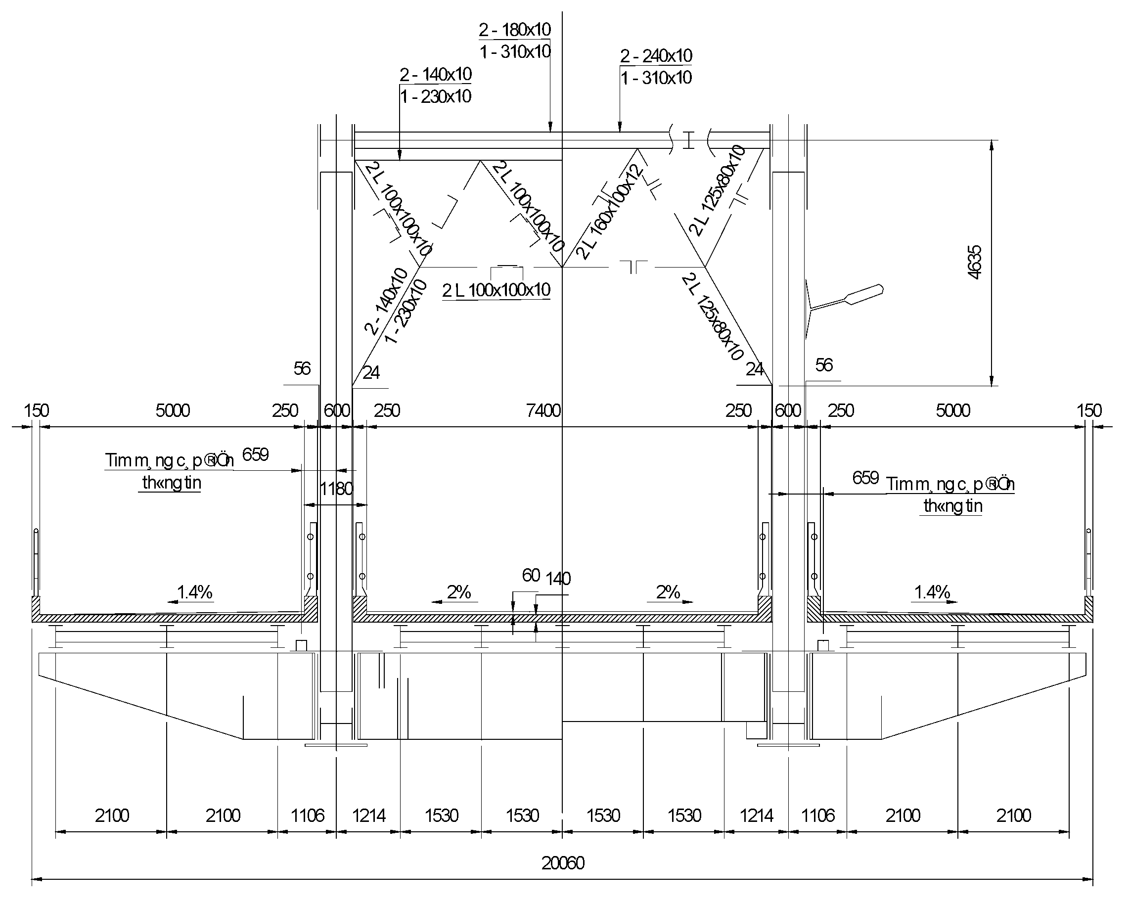
The entire width of the bridge is 20.06m (Figure 3). The bridge carries a four-lane bridge: two lanes in the middle for cars and buses, others for motorcycles. The bridge is designed with a load of H-30 on the main lane and H-6 on both sides of the cantilever. In the first days of being put into operation, this bridge had 7000-8000 traffic turns per day. But now, the number of vehicles crossing the bridge has increased dramatically, reaching tens of thousands of vehicles per day.

The main truss rods have an H-shaped cross section, the height depends on the position (see Table 2 for the details). At the truss nodes, a 32mm thick panel is used to connect the truss ends

3.2. On-Site Measurement Campaign before Damage

a.: Description of experiment

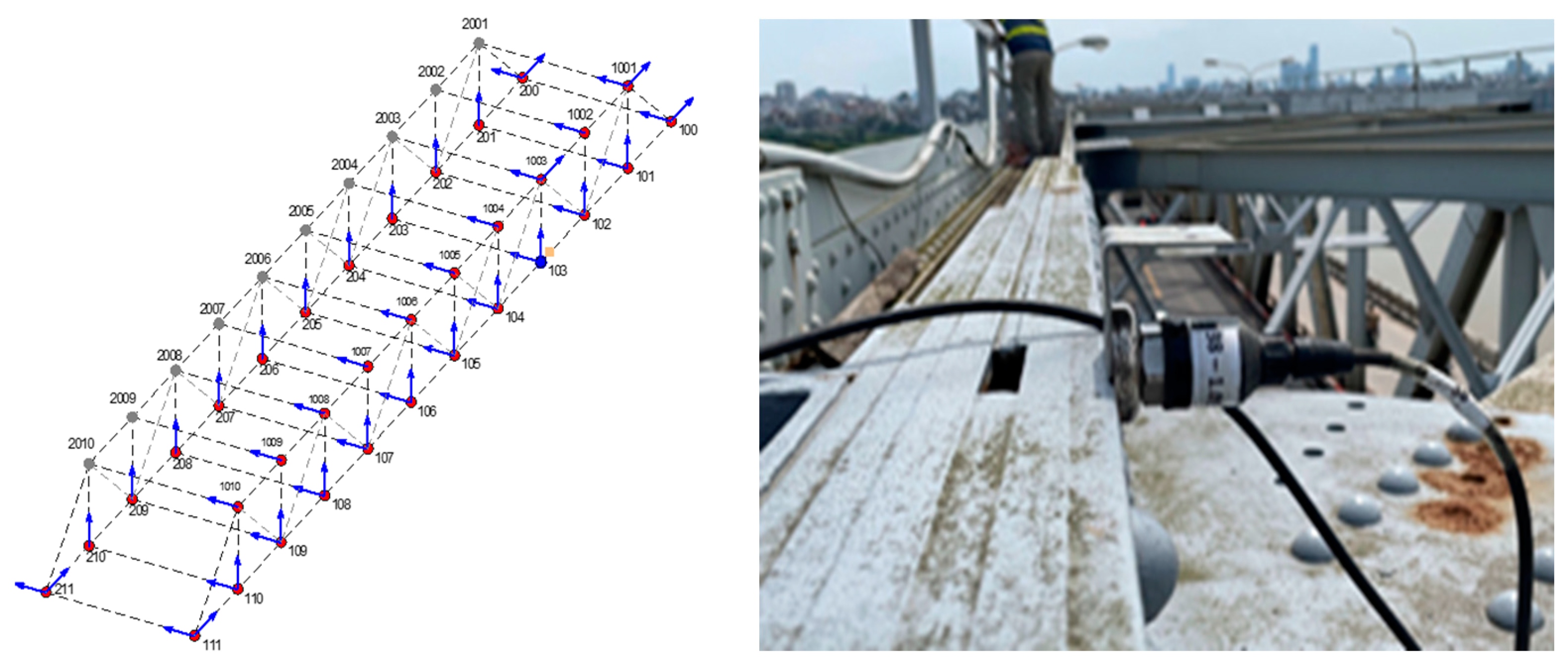
In the framework of this study, a comprehensive survey and measurement campaign was carried out on span 08 of Chuong Duong bridge. The campaign includes geometric surveys and vibration measurements of the entire span 08. After finishing the geometric survey, conduct vibration measurement under random stimuli (wind, current, surrounding loads, vehicles crossing the bridge, among others). Eight highly sensitive sensors, ranging in sensitivity from 1054 to 1083mV/m/s2 were used. With a sampling frequency of 1651 Hz, each setup’s average acquisition time was 30 minutes. Due to a shortage of sensors and in order to determine the global vibration modes of the bridge. To achieve the vibration modes of the entire span, a measuring grid of 34 points covering all truss nodes was established. However, due to the limited number of sensors, the measuring grid is divided into 8 setups (Figure 4). The reference point at node 103 is selected to link the data from the sensors. Other moving points are located at truss nodes on the bridge. The measurement procedure is controlled by a laptop, which also gathers and saves dynamic responses.

In space, the Cartesian coordinate system is used to determine the direction of each measuring point. The x-axis is in the longitudinal direction, the y-axis is in the bridge’s transverse direction, and the z-axis is vertical with a positive upward direction. Two sensors with x and y axes were mounted at each bearing. The sensors were positioned on the y-axis, z-axis, or both y and z-axis at other points.

b.: Data processing and feature extraction

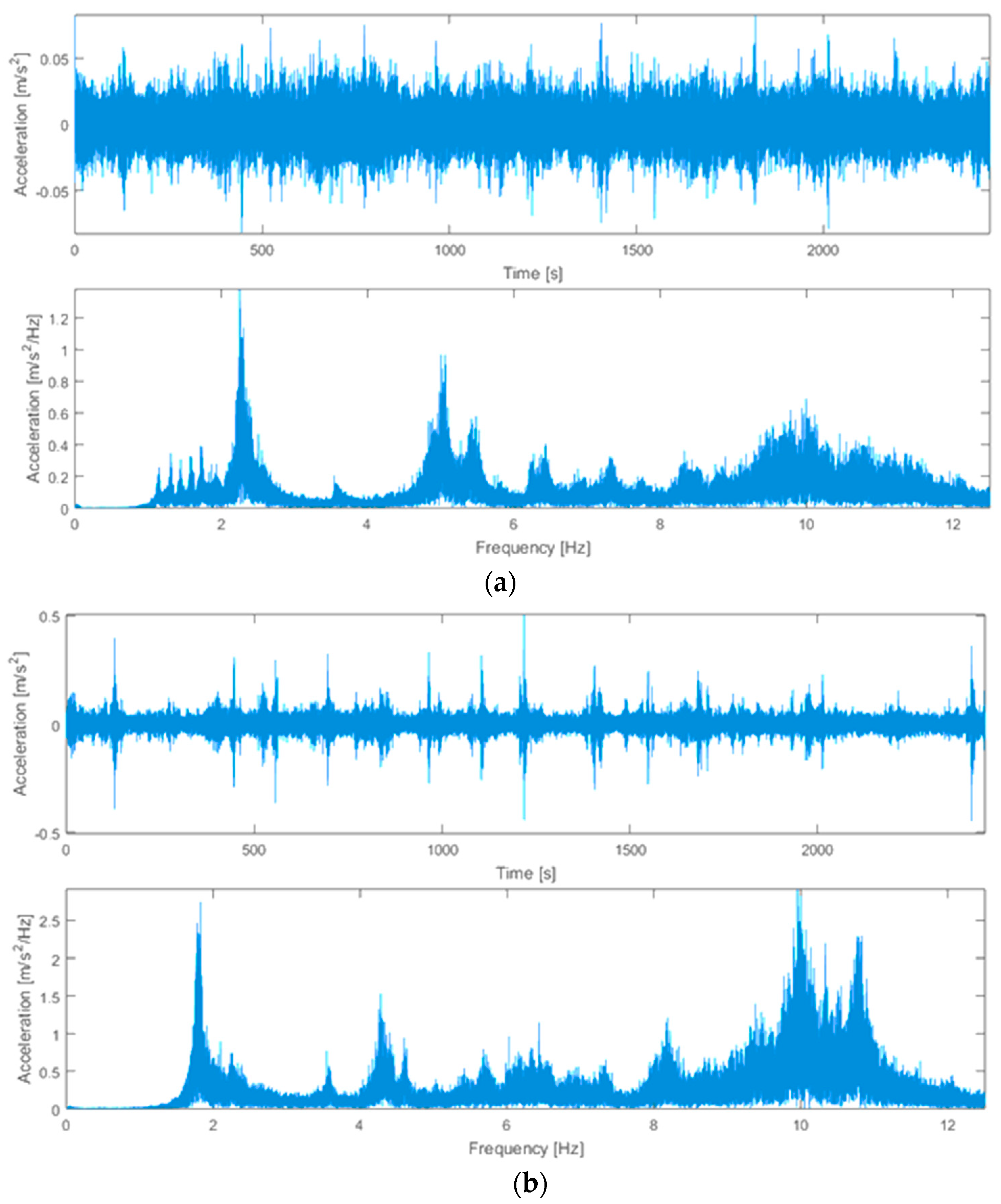
The MACEC toolbox [46] was used to analyze all of the measurement data. First, the data needs to be pre-processed. A measuring grid is created on the MACEC system. The measuring points are assigned and numbered, corresponding to the actual measuring points. Assign input parameters such as sensor label, sensitivity, data and measure to each measuring point. The measured signal data is often skewed and does not coincide with the balance axis; the remove-offset function removes these components from the measurement data. The obtained dynamic signal was taken from the time domain and represented in the frequency domain using the Fast Fourier Transform (FFT) (Figure 5).

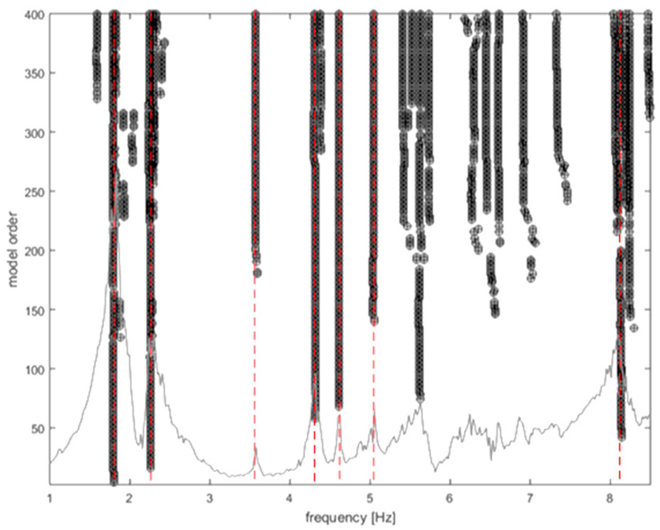
Based on input data and data obtained from pre-processing (noise removal, data classification into corresponding nodes), a model with complete data for measurement points is formed. System identification is accomplished using the covariance-based stochastic subspace identification (SSI-COV) technique. Based on knowledge from numerous similar constructs, the following criteria were selected to concretize and characterize the modality: frequency stabilization (1%), damping ratio stabilization (5%), and mode shape stabilization (1%). The stabilization diagrams (Figure 6) are constructed. The choice of stable poles (in red dash-line) were based on their obvious appearance in 8 setups.

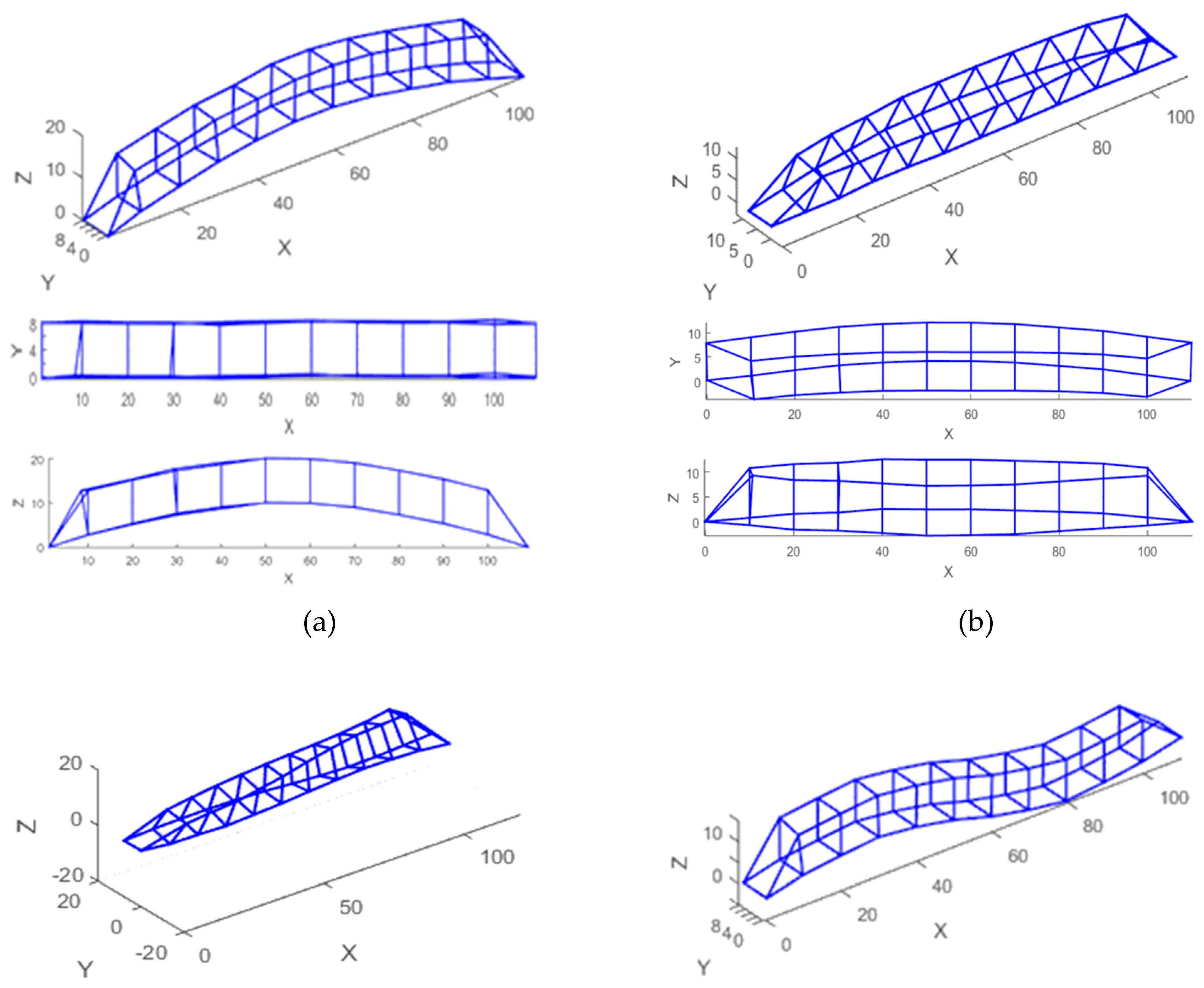
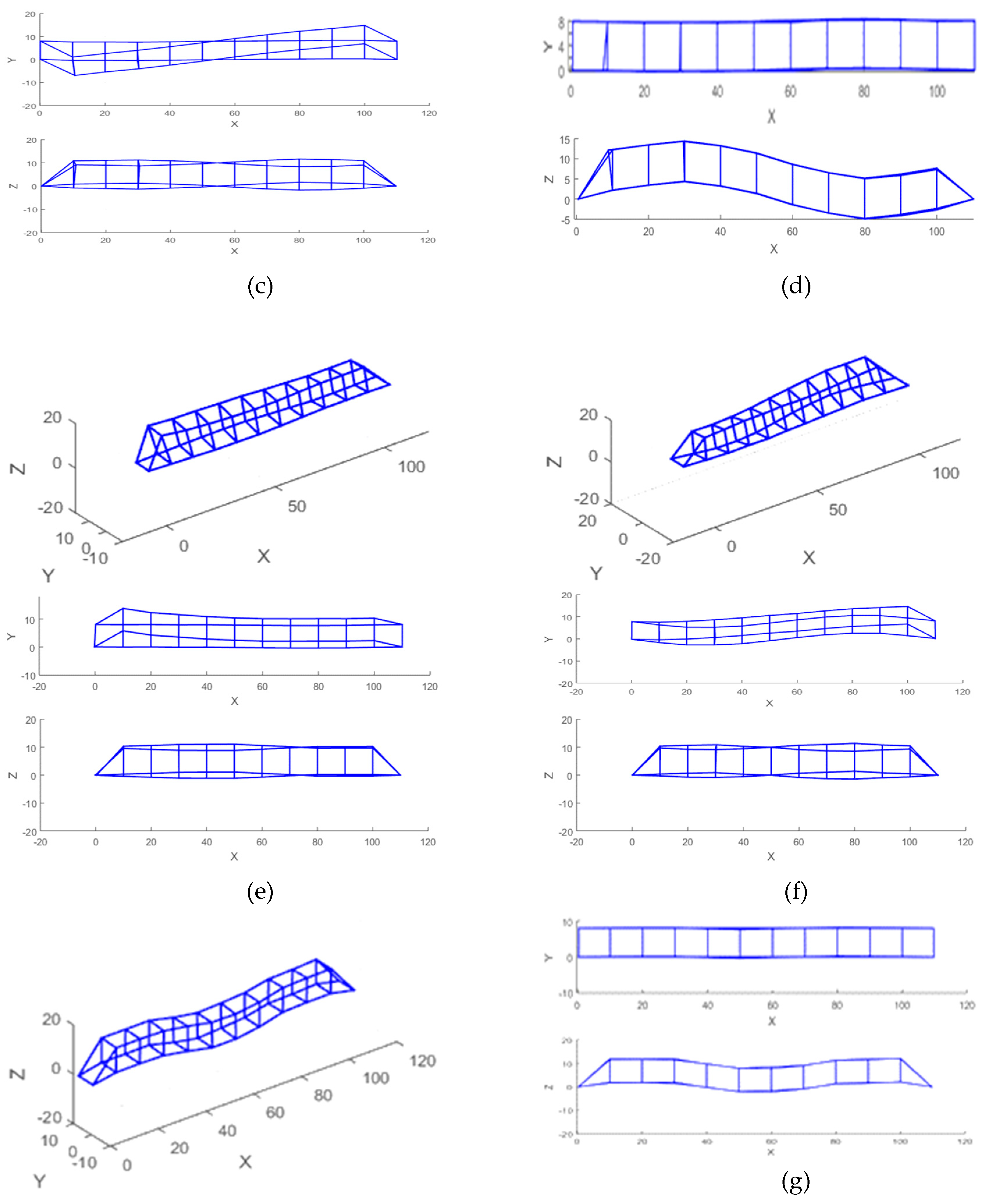
After data processing, seven identified modes shape is identified from the campaigns. Figure 7 displays mode shapes from 8 setups:

From the different setups, 7 modes could be identified. Their natural frequencies and damping ratios can be found in the Table 1.

The standard deviation of the natural frequency is calculated to assess the defined modes’ effectiveness. Because the values of std.f are low, each setting’s system recognition quality is high. Modal phase alignment (MPC) measures the mode shape’s departure from actual values, MPC=1 corresponds to the pure real mode. Every MPC value is higher than 0.998. A structure with light and/or proportional damping physics modes is likely to be realistic, so the elevated MPC result typically indicates a mode that has been precisely defined.

3.3. FEM Creation and Updating

Initial FE model

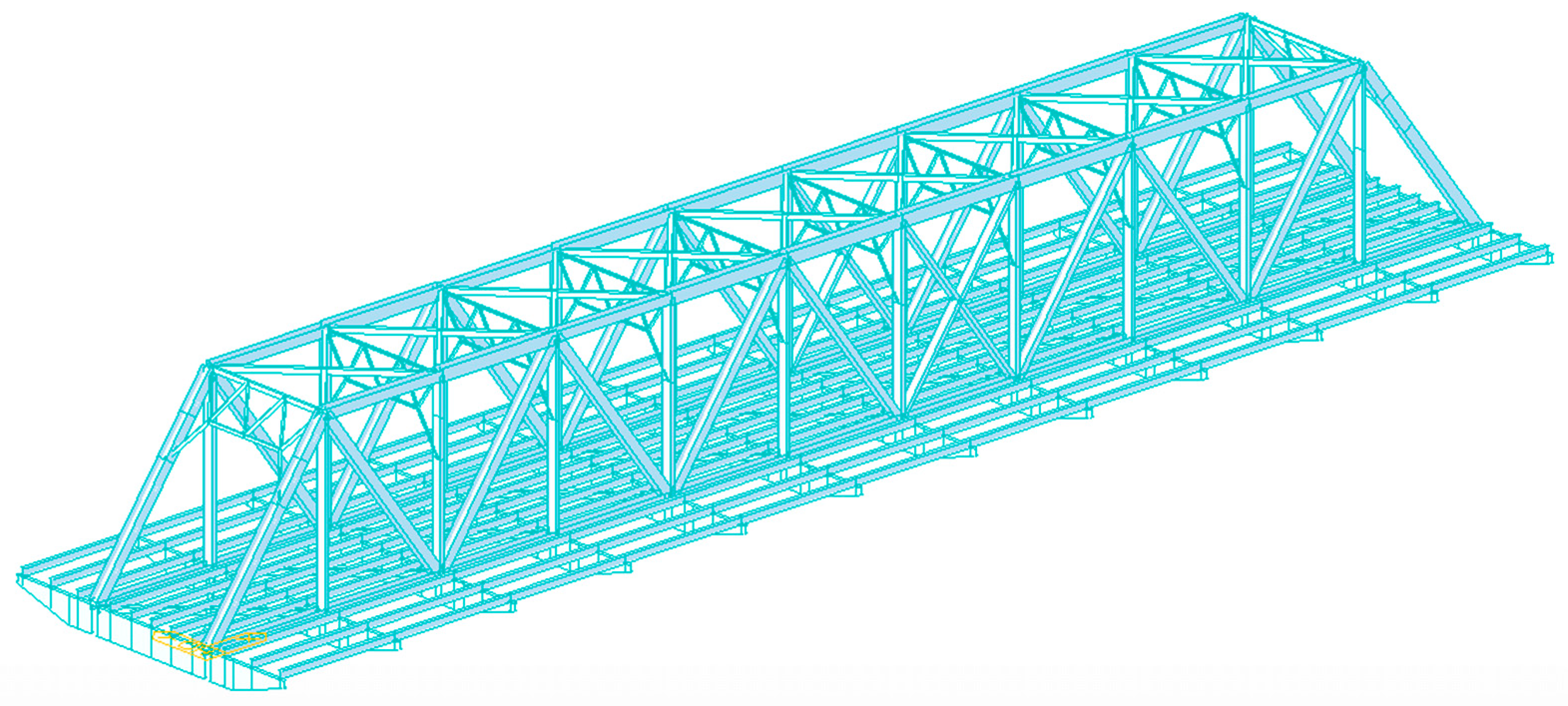
A FE model of Chuongduong bridge is built while taking into account the bridge’s structure (Figure 8). Top chords, bottom chords, cantilevers, gate frames, and verticals, all of which were modeled using three-dimensional beam elements, make up the principal structural components. Other components such as wind bracing, stiffening frame, and longitudinal linkage are modeled with truss elements. The global X-axis of the bridge is in its longitudinal direction, the Z-axis is vertical, and the Y-axis is transverse (to the direction of the river flow). The built model consists of 619 elements, which includes 461 beam elements and 158 truss elements. Six degrees of freedom (DOF) are available for each element node, and these DOFs correspond to translational and rotational displacements in the X, Y, and Z axes.

The input parameters of the material (Young’s modulus, specific gravity) as well as of the section (area, moment of inertia) are referenced from the as-built records. Specifically: Young’s modulus of steel (beams, truss rods, cantilever) E_s = 200 Mpa; the density of steel ρs = 7850kg/m³. For non-structural elements such as bridge deck, balustrades, lighting systems, and plumbing are included in the model as additional mass. Typical cross-sections of some truss members are shown in Table 2.

Table 2. Cross-sectional of truss members.

No	Truss members	Area (mm²)	Moment of inertia I_y (mm⁴)	Moment of inertia I_z (mm⁴)
1	Bridge gate frame	4.27 $\times$ 10⁴	2.9 $\times$ 10⁹	1.15 $\times$ 10⁹
2	Top lateral bracing	4.75 $\times$ 10⁴	3.31 $\times$ 10⁹	1.75 $\times$ 10⁹
3	Bottom lateral bracing	4.75 $\times$ 10⁴	3.31 $\times$ 10⁹	1.75 $\times$ 10⁹
4	Struts	1.83 $\times$ 10⁴	1.03 $\times$ 10⁹	5.29 $\times$ 10⁷
5	Diagonal chords	4.17 $\times$ 10⁴	2.82 $\times$ 10⁹	1.04 $\times$ 10⁹
6	Vertical chords	1.83 $\times$ 10⁴	1.03 $\times$ 10⁹	5.29 $\times$ 10⁷
7	Top chords	1.83 $\times$ 10⁴	1.03 $\times$ 10⁹	5.29 $\times$ 10⁷
8	Bottom chords	1.83 $\times$ 10⁴	1.03 $\times$ 10⁹	5.29 $\times$ 10⁷

Boundary Conditions: The Dirichlet boundary conditions of the numerical model are created to accurately reflect the boundary conditions of the actual structure. The span of 8 bridges in Chuong Duong includes 2 types of bearings (Figure 8). Based on the survey results, the displacement constraints of the model are made corresponding to the actual displacement capacity of the bearing.

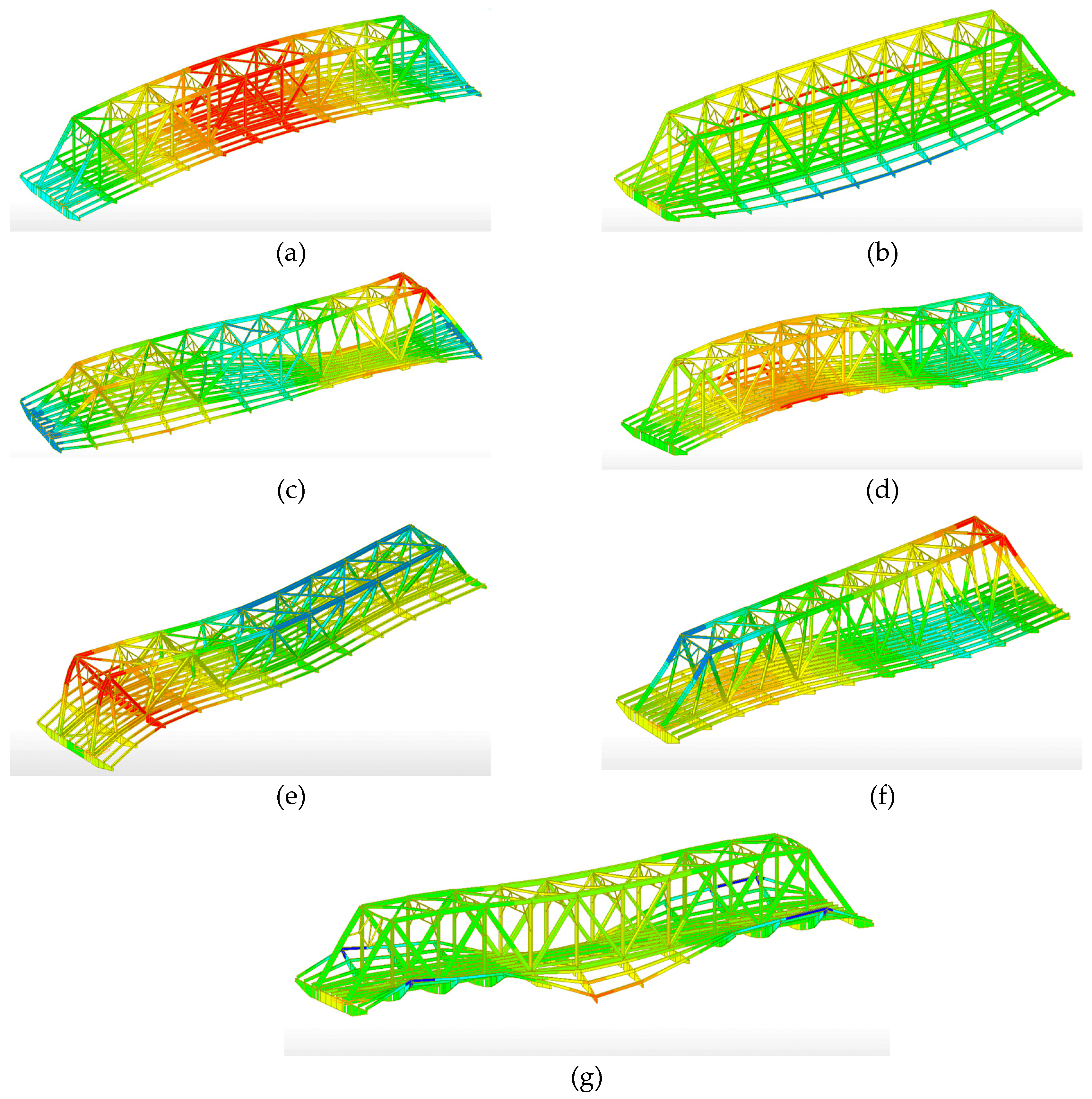
Utilizing the Block-Lancios method, The FE model’s dynamic analysis is carried out. Figure 10 and Table 3 displays some mode forms’ mode shapes and natural frequencies.

The Modal Assurance Criterion (MAC), a statistical indicator, is particularly sensitive to significant discrepancies in the mode shapes and is comparatively insensitive to smaller differences [47]. This results in a reliable statistical indication and consistency between the mode shapes. This study uses the MAC value to evaluate and update the finite element model. The formula 26 is used to calculate the MAC value:

M A C = \frac{{|\sum_{k = 1}^{n} {({\tilde{φ}}_{k})}^{T} \times φ_{k}|}^{2}}{\{\sum_{k = 1}^{n} {({\tilde{φ}}_{k})}^{T} \times φ_{k}\} \times \{\sum_{k = 1}^{n} {(φ_{k})}^{T} \times φ_{k}\}}

(26)

Where n is number of modes shape considered, MAC is modal assurance criterion, ϕ_k, 𝜑̃_k is modes shape FEM and experimental, ω_k ; ω;̃_k is frequencies FEM and experimental; T represents transposed matrix.

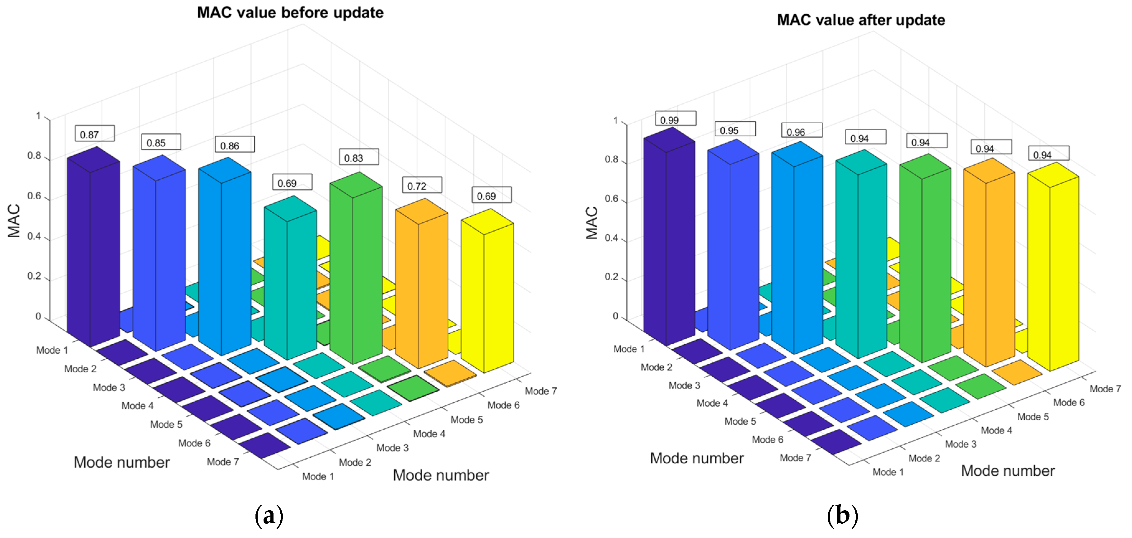
The MAC values are determined through formula (26) between the FE model results and the actual measurements. The first 3 MAC values greater than 0.85 show good agreement between each pair of mode shapes. However, other MAC values do not reach this minimum value. The correlation between the calculated and measured mode shape vectors are not guaranteed. The frequency values are also significantly different. This is a common situation for initial FE models, most of which have not been able to extract modes with high accuracy. Meanwhile, depending on the calculation requirements of the structure, some structures need high accuracy to structure health monitoring, diagnose damage, and make major predictions accuracy for maintenance. There are many uncertain parameters such as material properties, stiffness parameters. For this reason, it is recommended to perform a model update procedure to reduce errors.

b Update model parameters through particle swarm optimization (PSO) algorithm

The particle swarm optimization (PSO) algorithm was established and developed on the ideas of swarm intelligence to find solutions for optimization problems in a particular search space [48,49]. To understand the PSO algorithm better, observe a simple example of a flock of birds foraging. The foraging space is now the entire three-dimensional space. At the beginning of the search, the whole flock flies in a certain direction, it can be very random. However, after a while of searching, some individuals in the herd began to find a place to contain food. Depending on the amount of food just searched, the individual sends a signal to other individuals searching in the vicinity. This signal propagates throughout the population. Based on the information received, each individual will adjust its flight direction and speed in the direction of where there is the most food. Such communication is often viewed as a phenotype of herd intelligence. This mechanism helps the whole flock of birds to find out where there is the most food in the extremely large search space.

In swarm optimization, each particle searches a space by itself, remembering the best value, and informing other individuals. Other instances will receive the information and decide to continue the search or report its location so that other instances continue to act. So that, values in search space will be done quickly and accurately. There are two parameters that are particularly important, the location of an instance and the search velocity. These two parameters are expressed through the formulas for updating the position and updating the velocity of the instance:

x^{i} (t + 1) = x^{i} (t) + v^{i} (t + 1)

(27)

v^{i} (t + 1) = w v^{i} + C_{1} r_{1} (p^{i} (t) - x^{i} (t)) + C_{2} r_{2} (G_{bes t} - x^{i} (t))

(28)

Where xⁱ is the position of instance i at different times (t and t+1); vⁱ is the speed of individual i; w is the parameter of inertial weight; C1 and C2 represent the population’s cognitive coefficient; r₁ and r₂ are random numbers in the range 0,1]; pⁱ(t) is the best position of each individual; G_best is the best location of the entire population. Each individual is characterized by its velocity vector and its position in space.

To evaluate the similarity between the FE model and practical structure, an objective function is built based on the natural frequency and the mode shape of the structure:

F i t n e s s = \sum_{k = 1}^{n} [1 - M A C (φ_{k}, {\tilde{φ}}_{k})] + \sum_{k = 1}^{n} \frac{ω_{k}^{2}}{{\tilde{ω}}_{k}^{2}} = \sum_{k = 1}^{n} [1 - \frac{{({\tilde{φ}}_{k}^{T} φ_{k})}^{2}}{(φ_{k}^{T} φ_{k}) (φ_{k}^{T} {\tilde{φ}}_{k})}] + \sum_{k = 1}^{n} \frac{{(ω_{k} - {\tilde{ω}}_{k})}^{2}}{{\tilde{ω}}_{k}^{2}}

(29)

In the case of Chuong Duong bridge, determining material parameters requires many experiments. At the same time, the masses of non-structural parts are also difficult to determine accurately. Some uncertain parameters are selected to update the numerical model. Based on experience

The updated uncertainty parameters and FE model after using the PSO are presented in Table 5.

The results after updating show that updating the model lowers the discrepancy between the calculated and measured natural frequencies, and the MAC value reaches a good level.

The MAC values of the FE model before and after the update are shown in Figure 9. After being updated, the accuracy of the model has increased a lot. These MAC values show good agreement between the FE and the actual models.

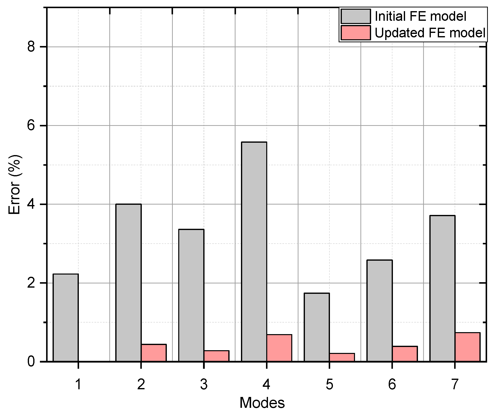
Figure 10 shows that before updating the model, the calculation results and natural frequency measurement results have high errors, after updating the model, the error of the natural frequency between calculation and measurement decreases significantly, the model is highly accurate and reliable.

The calculation results show that, after about 30 iterations performed by PSO, the model parameters begin to converge and give good results, minimizing the process of testing parameters in the modeling. After updating, the numerical model is accurate and almost the same as the actual object. This model is employed for creating data to train the ANN.

3.4. Generate Data and Train the ANN Model

a. Single damages

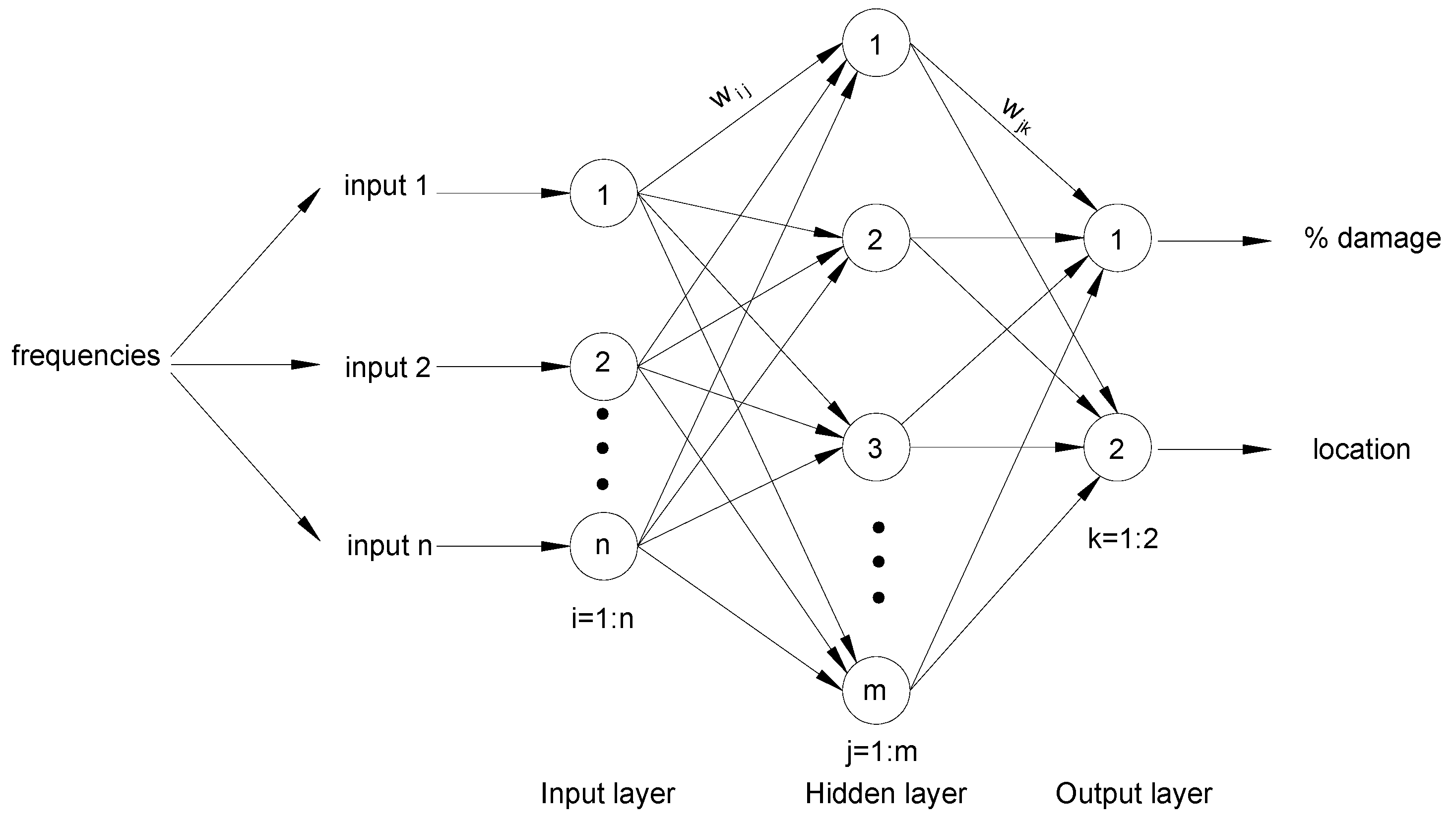
Three layers make up the ANN’s architecture in this work: an input layer, a hidden layer, and an output layer. The first seven modes’ frequencies are used as input data with various damage situations, and the output data comprises damage locations and levels (Figure 11).

The updated model’s modal analysis creates input and output data for the ANN. The elements’ stiffness is decreased to create scenarios of structural damage. With a 1% interval, the elements’ stiffness decreases from 0% to 50%. Damages are only truly dangerous and sensitive enough when they occur on major structural components. Therefore, only the main truss rods are considered in this case. The equation determines the quantity of input data needed to train the network:

N = n_{e} \times n_{s}

(30)

Where: n_e – total of elements is considered, n_s - the number of damage scenarios occurring for a single element. Consider 84 main elements of the truss. The input data will consist of 4200 samples

The ANN is configured to the settings for training the network after the data generation. The results of the network training process are significantly influenced by the number of neurons in the hidden layer. If the ANN has too few hidden layers, the ANN is too simple and difficult to deal with the problems to be solved. In contrast, ANN has too many hidden layers, the network is too complicated. Computer resources consume a lot, easily leading to overfitting. The loop is used to choose the ideal number of hidden layers. Within the range of 1 to 50, the number of hidden layers that will be selected by the loop. Additionally, the impact of noise is evaluated in all situations with a level of 2% for natural frequencies. The Levenberg-Marquardt backpropagation algorithm is used by the ANN to train the network. For damage identification, data split in the training procedure by 70%-15%-15% is used. There are a maximum of 1000 epochs. In the case of epochs greater than 1000 but still not reaching the best value, it is necessary to implement network optimization solutions.

After training, the following figures demonstrate how the ANN model performed:

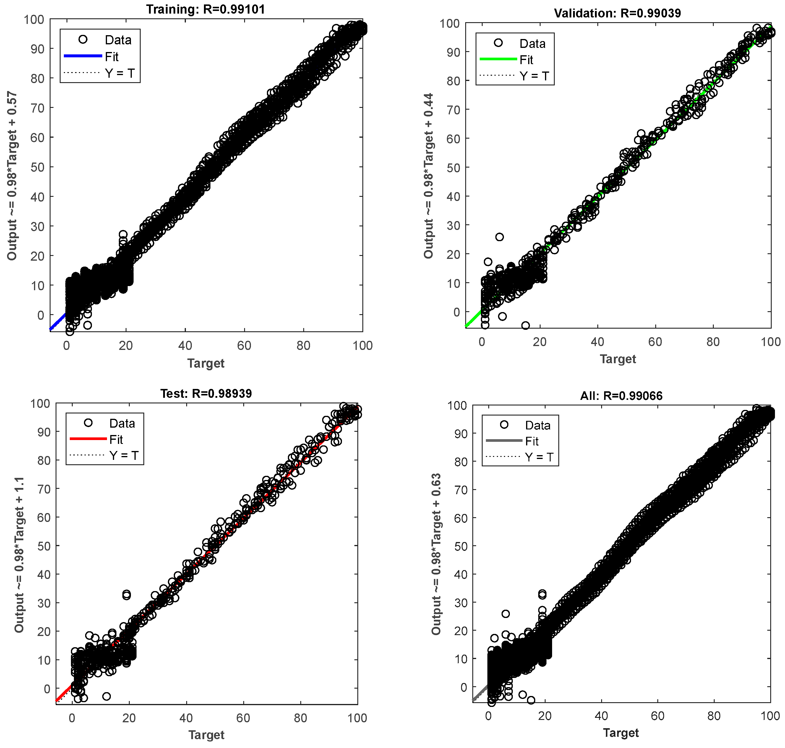
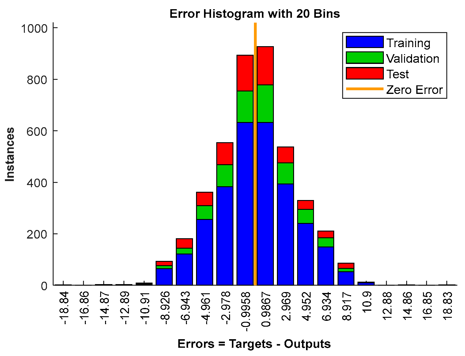
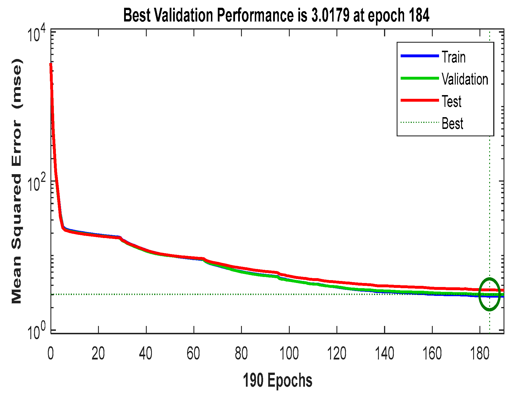
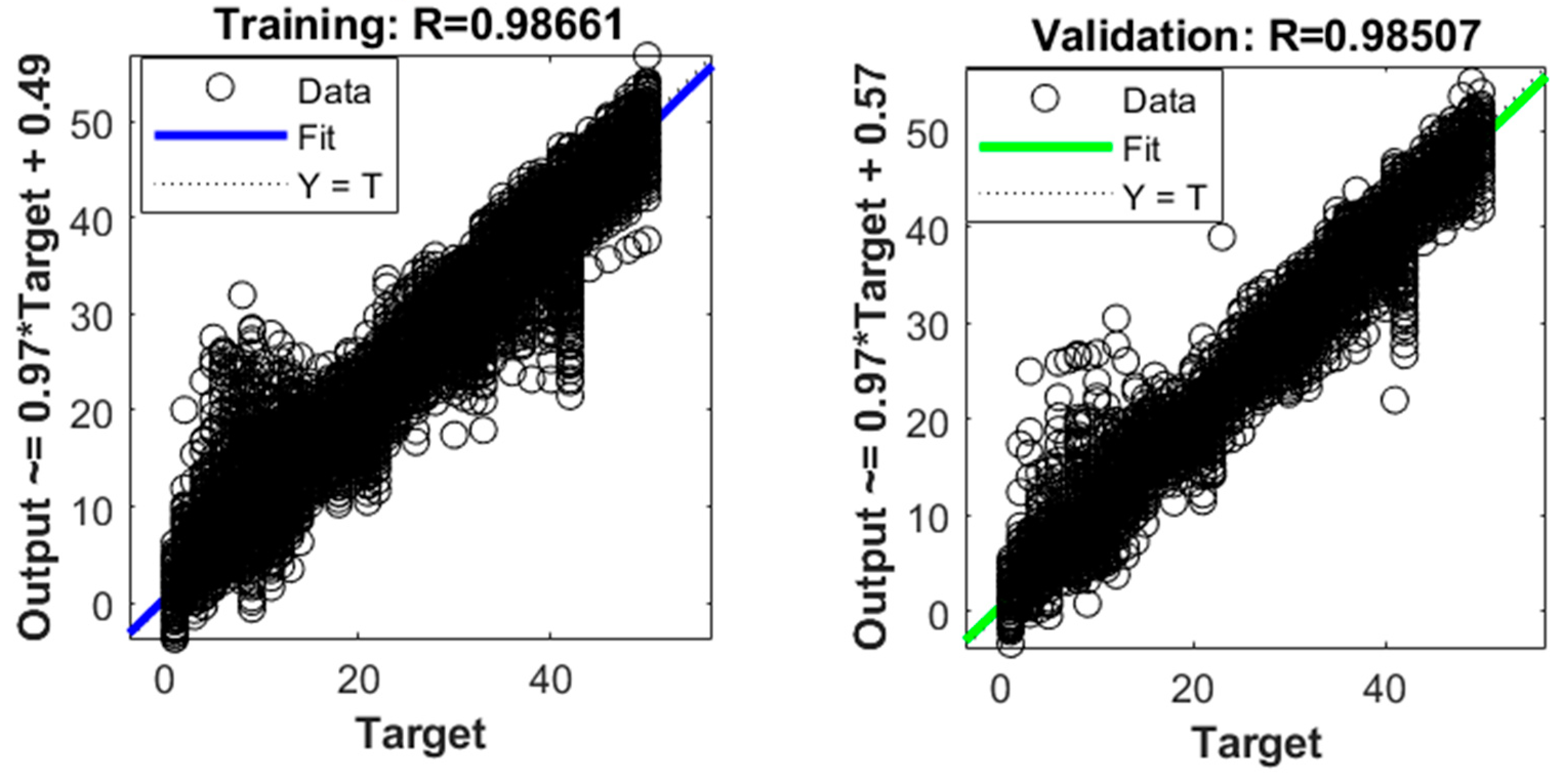
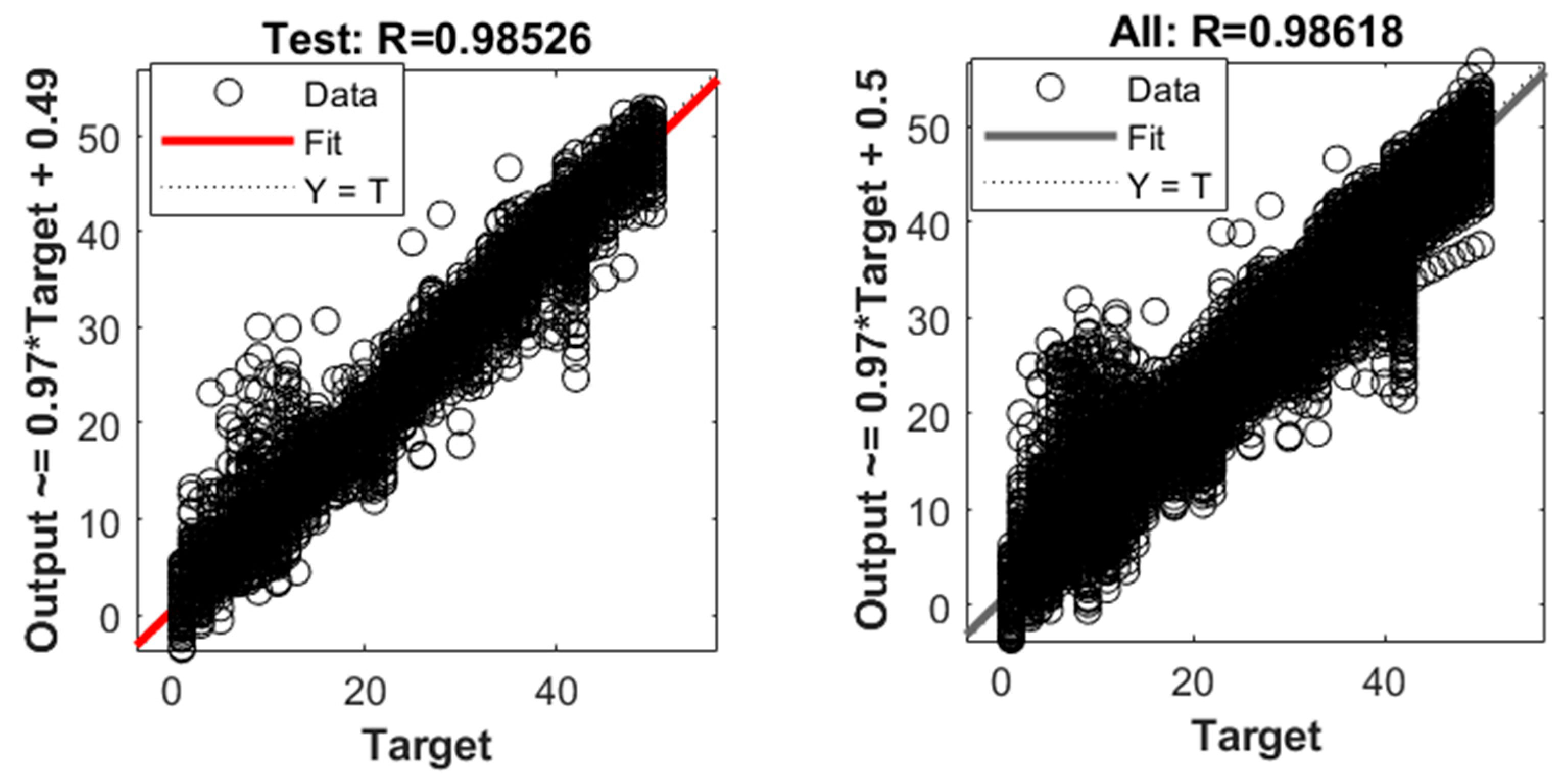
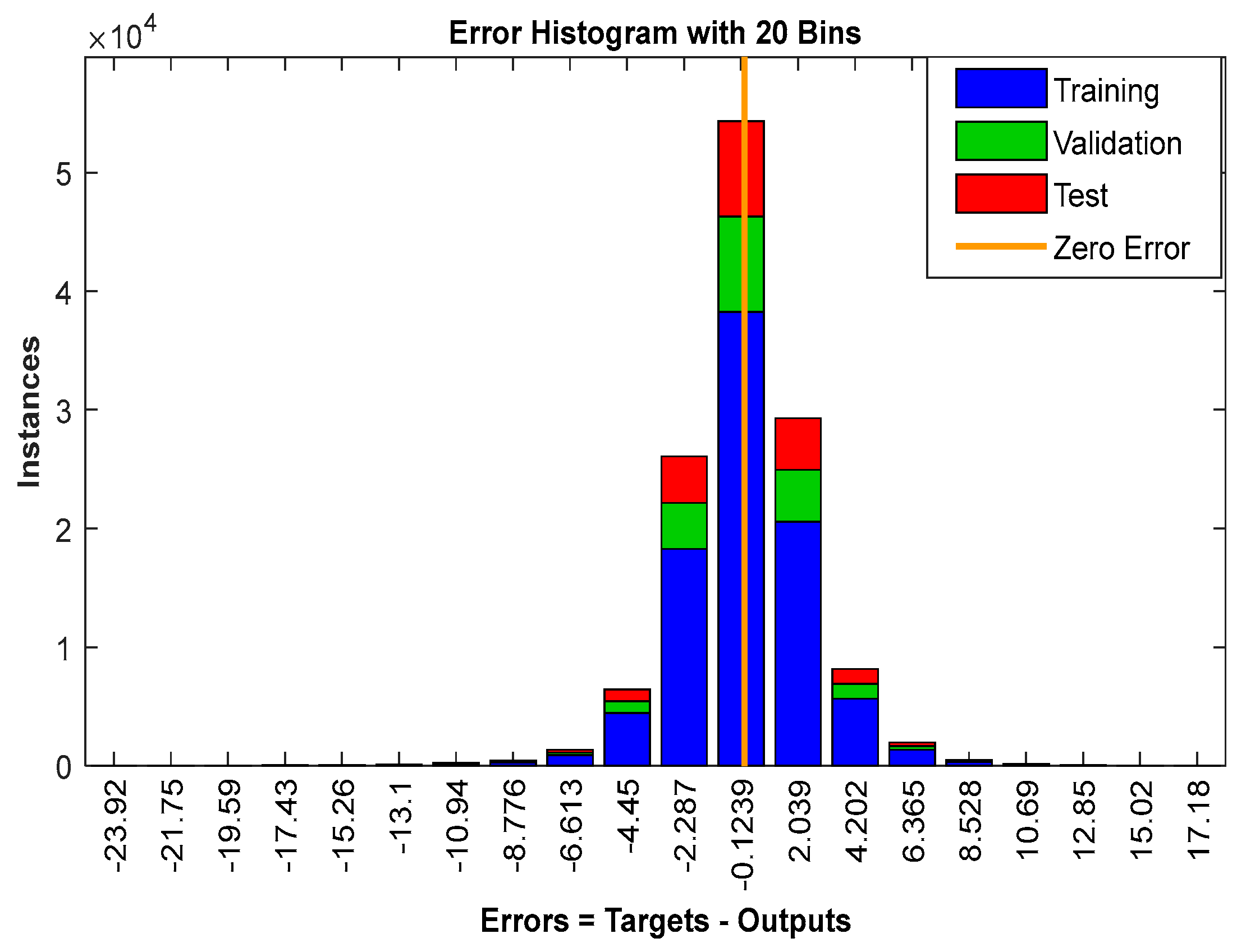
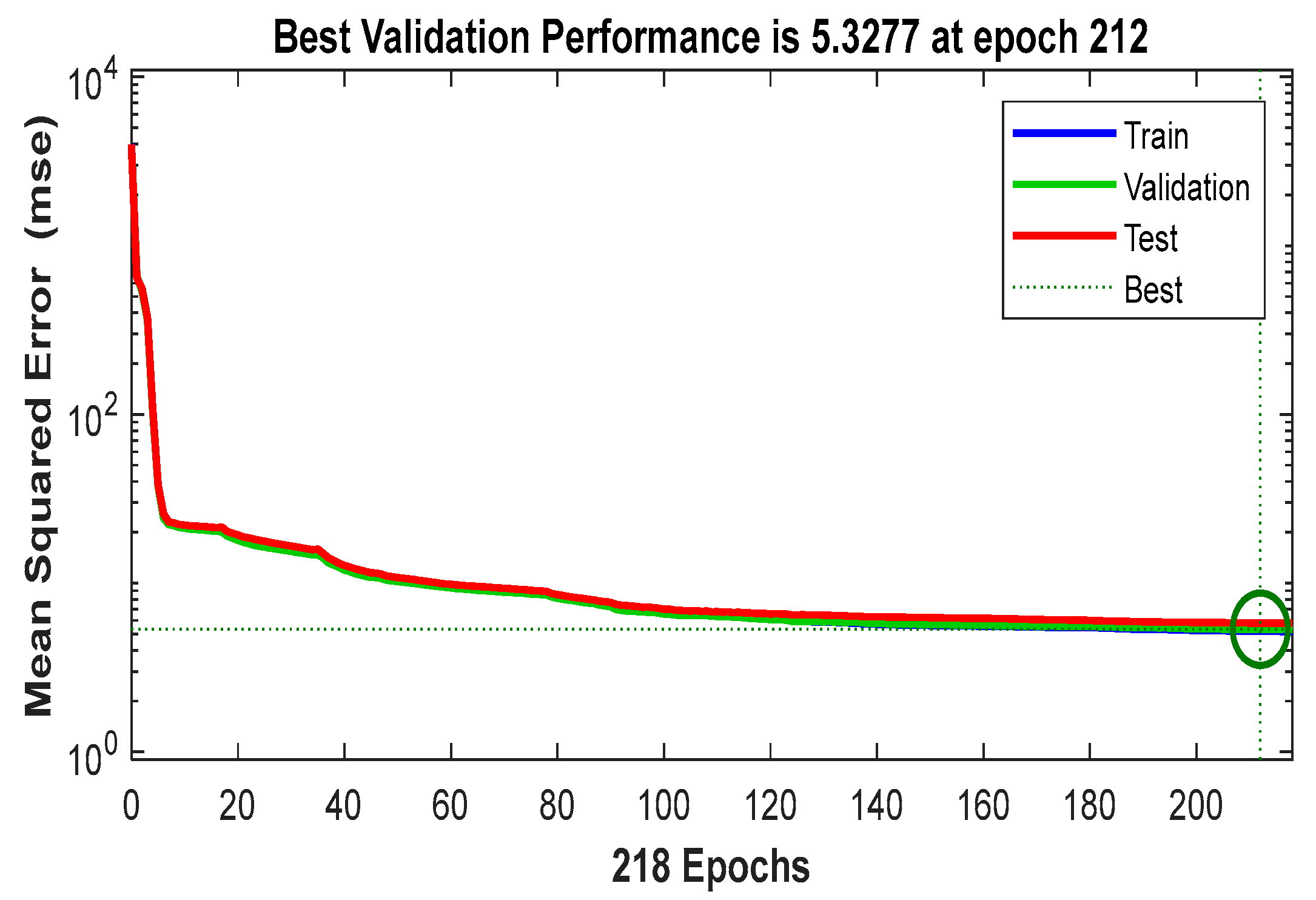
All training cases with regression values more than 0.99 are displayed in Figure 12. The training, evaluation, and test datasets are located along the target line (45degree line). This demonstrates that the real value and predicted value are almost similar. The regression values (R) in linear regression models always range from 0 to 1. The estimated and desired outcomes are the same if R is near to the upper bound (1). Figure 13 shows the histogram of the calculated and intended output errors. There is extremely little variance between the target and the output. Figure 14 shows the training performance in the datasets. The best validation performance value of 3.0179 is achieved at epoch 190. Epoch number does not exceed 1000, network optimization is not necessary. The graph also shows that the values in the data sets are quite convergent, no overfitting phenomenon occurs. From the performance graph of R-values, MSE (Tolerance), error histogram, the model has clearly been successfully trained, which can be used to apply to the contruction

b. 2 damaged elements

Damages are simultaneously generated by two random elements. For each element, a damage level is assigned from 0% to 50% with a 1% interval. In this study, the failures at the elements are assumed to be the same. The amount of data is calculated according to the formula:

N = n_{s} \times \frac{n_{e}!}{2! \times (n_{e} - 2)!}

(31)

The total amount of data generated is: 174300 samples

Figure 15 shows that

R

– values of the network using ANN is 0.986. The training, validation, and test datasets follow the regression line.

According to Figure 16 and Figure 19, there are small deviations from the zero error line between computed and desired values. Results obtained show that a good agreement between predicted and actual outputs.

3.5. The Service of the Trained ANN Model in Actual

a. Single damage

Normally, to detect and locate the damage of the bridge structure, a comprehensive survey investigation will be carried out. After the survey, experts will make a computational model and evaluate. This work requires a lot of human resources and costs a lot of money. Only consider measuring the vibration of the entire span structure, the implementation of the setups measurements as described above also requires a lot of work. Instead, using an artificial neural network offers a huge advantage.

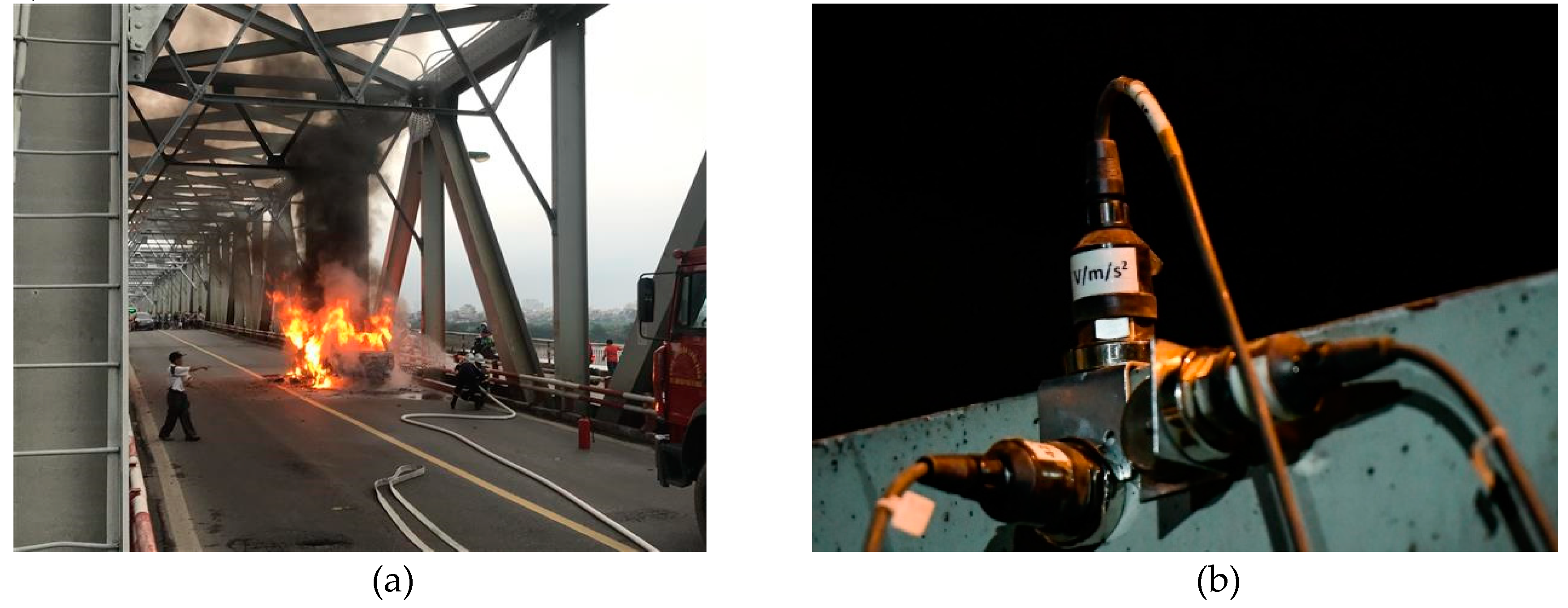
Using a trained network applied to the actual span structure of Chuong Duong bridge. During the service, there was an accident on Chuong Duong bridge that affected the bridge structure (Figure 18).

A simple experiment was conducted since only the structure’s natural frequency needs to be ascertained. A single vibration measurement point in 3 directions is located on Chuong Duong bridge (Figure 18). With only 1 measuring point, the natural frequency of Chuong Duong bridge has been identified. Although it is not possible to identify the mode shapes of the bridge, with the trained ANN it is possible to locate and quantify the damage.

The results of the nature frequencies of the first 7 mode shapes determined through the experiment are [1.229; 2.4167; 4.1954; 4.2623; 4.5925; 6.2147; 7.7865]. This result is used as input to feed the trained network. Results after putting data into the network return [25; 6]. This means that 25% damage is detected at element 6 (truss number 6). It is easy to see that the result of locating damage at element 6 is correct. According to the report of the UCT company who performed the calculation of damage assessment, damage level of truss rod is 30%. Results using ANN are relatively accurate. This is a case of damage that is easy to identify and recognize in practice. However, for cases where the damage location is difficult to detect (for example, the damaged location is located in too high, difficult to reach locations, in the middle of the river), the ANN will show its advantages.

b. 2 damaged elements

In this case, a hypothetical failure is generated on the updated finite element model. Two elements 10 and 15 are assumed to be 40% damaged. Put the data into the trained ANN model, the network detects and returns the result 39% and occurs at element 10 and 15. Although not 100% accurate, the trained network detected the location and was relatively close to the simulation results.

4. Conclusions

This study approaches artificial intelligence-based structural health monitoring. Through testing and practical application in a steel truss bridge, it achieves potential performance in terms of structural monitoring. Along with the detailed explanation in this paper, some main conclusions can be derived:

Before applying the ANN algorithm, an accurate (or relatively accurate) data source is required. This can be performed by creating a finite element model for extracting input data. However, if it is applied to actual works, it is necessary to have measures to update the model. In this study, particle swarm optimization (PSO) is used. Therefore, FEM can turn closer to the real behavior of the structures.
Creating and organizing data from a finite element model is very important if want to get good results when training ANNs. With a large number of samples, training the network takes time, but the effect after training can make up for this.
With the use of a trained ANN, failures can be detected and quantified. The proposed application results in a well-establishment with the actual test from an under-operating bridge.
Compared with other methods, this approach has various advantages: saving human resources, being able to identify damage in hard-to-detect locations, and reducing the number of measuring points in the case of vibration tests.
In the case study of this research, with a single failure, the ANN was able to identify and quantify the damage relatively accurately. For damage occurring on 2 elements, since there is no actual data, the network usage after training is done on the model. The results are quite satisfactory. The case where the data of 2 simultaneous damages seems to be more accurately predicted by the network. This can be explained because actual experimental data will more or less have noise, and at the same time affected by many factors. Meanwhile, the data used to confirm the case of 2 damages at the same time is taken directly from the model

Author Contributions

“Conceptualization, M.T., J.M. and H.S.; methodology, M.T., J.M., and H.N.; software, M.T., B.N., and S.D.; validation, J.M. and S.D.; formal analysis, Q.N.; investigation, E.B., M.T. and S.D.; resources, E.B.; data curation, S.D.; writing—original draft preparation, M.T. and S.D.; writing—review and editing,M.T., J.M. and S.D.; visualization, B.N. and M.T..; supervision, J.M., H.S., H.N. and T.N.; project administration, J.M. and S.D.; funding acquisition, J.M., E.B. and S.D. All authors have read and agreed to the published version of the manuscript.”

Acknowledgments

This work was partly financed by FCT / MCTES through national funds (PIDDAC) under the R&D Unit Institute for Sustainability and Innovation in Structural Engineering (ISISE), under reference UIDB / 04029/2020, and under the Associate Laboratory Advanced Production and Intelligent Systems ARISE under reference LA/P/0112/2020 and financial support of the project research “B2022-GHA- 03” of the Ministry of Education and Training. The authors also acknowledge ANI (“Agência Nacional de Inovação”) for the financial support given to the R&D Project “GOA Bridge Management System – Bridge Intelligence”, with reference POCI-01-0247-FEDER-069642, cofinanced by European Regional Development Fund (FEDER) through Operational Competitiveness and Internationalization Program (POCI). Minh Tran was supported by the doctoral Grant reference PRT/BD/154268/2022 financed by Portuguese Foundation for Science and Technology (FCT), under MIT Portugal Program (2022 MPP2030-FCT). Helder S.Sousa acknowledges the funding by FCT through the Scientific Employment Stimulus - 4th Edition.

Conflicts of Interest

Declare conflicts of interest or state “The authors declare no conflict of interest.”

References

Encardio Rite Group [Updated] A Guide on Geodetic Survey and Monitoring - Encardio Rite. Available online: https://www.encardio.com/blog/a-guide-on-geodetic-survey-and-monitoring (accessed on 30 May 2023).
Beshr, A.A.E.-W. Structural Deformation Monitoring and Analysis of Highway Bridge Using Accurate Geodetic Techniques. Engineering 2015, 07, 488–498. [Google Scholar] [CrossRef]
Eteje, S.O. Detailed Geodetic Technique Procedures for Structural Deformation Monitoring and Analysis. International Journal of Scientific and Technological Research 2020. [Google Scholar] [CrossRef]
Liu, S.; Liu, X.; Yang, F. Control Surveying and Structural Health Monitoring Applied in Large Bridge. Adv Mat Res 2013, 639–640, 243–246. [Google Scholar] [CrossRef]
Lienhart, W. Geotechnical Monitoring Using Total Stations and Laser Scanners: Critical Aspects and Solutions. J Civ Struct Health Monit 2017, 7, 315–324. [Google Scholar] [CrossRef]
Segalini, A.; Carri, A.; Savi, R. Role of Geotechnical Monitoring: State of the Art and New Perspectives. In Proceedings of the GEO-EXPO; Drustvo za geotehniku u Bosni i Hercegovini, October 10 2017; pp. 19–26. [Google Scholar]
Viola, E.; Bocchini, P. Non-Destructive Parametric System Identification and Damage Detection in Truss Structures by Static Tests. Structure and Infrastructure Engineering 2013, 9, 384–402. [Google Scholar] [CrossRef]
Ugalde, U.; Anduaga, J.; Martinez, F.; Iturrospe, A. A SHM Method for Detecting Damage with Incomplete Observations Based on VARX Modelling and Granger Causality. 2016.
Martínez, D.; Obrien, E.J.; Sevillano, E. Damage Detection by Drive-by Monitoring Using the Vertical Displacements of a Bridge. Insights and Innovations in Structural Engineering, Mechanics and Computation - Proceedings of the 6th International Conference on Structural Engineering, Mechanics and Computation, SEMC 2016, 2016; 1915–1918. [Google Scholar] [CrossRef]
Hjelmstad, K.D.; Shin, S. Damage Detection and Assessment of Structures from Static Response. J Eng Mech 1997, 123, 568–576. [Google Scholar] [CrossRef]
Bakhtiari-Nejad, F.; Rahai, A.; Esfandiari, A. A Structural Damage Detection Method Using Static Noisy Data. Eng Struct 2005, 27, 1784–1793. [Google Scholar] [CrossRef]
Doebling, S.W.; Farrar, C.R.; Prime, M.B. A Summary Review of Vibration-Based Damage Identification Methods. The Shock and Vibration Digest 1998, 30, 91–105. [Google Scholar] [CrossRef]
Salawu, O.S. Detection of Structural Damage through Changes in Frequency: A Review. Eng Struct 1997, 19, 718–723. [Google Scholar] [CrossRef]
Khatir, S.; Khatir, T.; Boutchicha, D.; Le Thanh, C.; Tran-Ngoc, H.; Bui, T.Q.; Capozucca, R.; Abdel-Wahab, M. An Efficient Hybrid TLBO-PSO-ANN for Fast Damage Identification in Steel Beam Structures Using IGA. Smart Struct Syst 2020, 25, 605–617. [Google Scholar] [CrossRef]
Farrar, C.R.; Doebling, S.W. Damage Detection and Evaluation II. Modal Analysis and Testing 1999, 345–378. [Google Scholar] [CrossRef]
Carden, E.P.; Fanning, P. Vibration Based Condition Monitoring: A Review. 2004, 3, 355–377. [Google Scholar] [CrossRef]
Catbas, F.N.; Brown, D.L.; Aktan, A.E. Use of Modal Flexibility for Damage Detection and Condition Assessment: Case Studies and Demonstrations on Large Structures. Journal of Structural Engineering 2006, 132, 1699–1712. [Google Scholar] [CrossRef]
Alvandi, A.; Cremona, C. Assessment of Vibration-Based Damage Identification Techniques. J Sound Vib 2006, 292, 179–202. [Google Scholar] [CrossRef]
Nhung, N.T.C.; Minh, T.Q.; Matos, J.C.; Sousa, H.S. Research and Application of Indirect Monitoring Methods for Transport Infrastructures to Monitor and Evaluate Structural Health. 2021.
Mazurek, D.F.; Mazurek; F. , D. Modal Sensitivity to Damage in Multigirder Bridges. SPIE 1997, 3089, 1892. [Google Scholar]
Doebling, S.; Farrar, C. Statistical Damage Identification Techniques Applied to the I-40 Bridge over the Rio Grande River. 1998.
Alvandi, A. Contribution à l’utilisation Pratique de l’évaluation Dynamique Pour La Détection d’endommagements Dans Les Ponts. 2003.
Doebling, S.W.S.; Farrar, C.R.C.; Prime, M.B.M.; Shevitz, D.W.D. Damage Identification and Health Monitoring of Structural and Mechanical Systems from Changes in Their Vibration Characteristics: A Literature Review. Los Alamos National Laboratory 1996. [Google Scholar] [CrossRef]
Karbhari, V.M.; Lee, L.S.W. Vibration-Based Damage Detection Techniques for Structural Health Monitoring of Civil Infrastructure Systems. Structural Health Monitoring of Civil Infrastructure Systems 2009, 177–212. [Google Scholar] [CrossRef]
Farrar, C.R.; Doebling, S.W.; Nix, D.A. Vibrationbased Structural Damage Identification. Philosophical Transactions of the Royal Society of London. Series A: Mathematical, Physical and Engineering Sciences 2001, 359, 131–149. [Google Scholar] [CrossRef]
Khiem, N.T.; Lien, T. V. A Simplified Method for Natural Frequency Analysis of a Multiple Cracked Beam. J Sound Vib 2001, 245, 737–751. [Google Scholar] [CrossRef]
Nguyen, T.; Chan, T.H.T.; Thambiratnam, D.P. Field Validation of Controlled Monte Carlo Data Generation for Statistical Damage Identification Employing Mahalanobis Squared Distance. 2014, 13, 473–488. [Google Scholar] [CrossRef]
Zhang, Z.; Shankar, K.; Morozov, E. V.; Tahtali, M. Vibration-Based Delamination Detection in Composite Beams through Frequency Changes. 2014, 22, 496–512. [Google Scholar] [CrossRef]
Jeong, M.-J.; Choi, J.-H.; Koh, B.-H. Isomap-Based Damage Classification of Cantilevered Beam Using Modal Frequency Changes. 2014.
Gillich, G.R.; Ntakpe, J.L.; Abdel Wahab, M.; Praisach, Z.I.; Mimis, M.C. Damage Detection in Multi-Span Beams Based on the Analysis of Frequency Changes. J Phys Conf Ser 2017, 842, 012033. [Google Scholar] [CrossRef]
Wang, L.; Lie, S.T.; Zhang, Y. Damage Detection Using Frequency Shift Path. Mech Syst Signal Process 2016, 66–67, 298–313. [Google Scholar] [CrossRef]
Sha, G.; Radzieński, M.; Cao, M.; Ostachowicz, W. A Novel Method for Single and Multiple Damage Detection in Beams Using Relative Natural Frequency Changes. Mech Syst Signal Process 2019, 132, 335–352. [Google Scholar] [CrossRef]
Khan, M.W.; Din, N.A.; Ul Haq, R. Damage Detection in a Fixed-Fixed Beam Using Natural Frequency Changes. Vibroengineering PROCEDIA 2020, 30, 38–43. [Google Scholar] [CrossRef]
He, K.; Zhu, W.D. Structural Damage Detection Using Changes in Natural Frequencies: Theory and Applications. J Phys Conf Ser 2011, 305. [Google Scholar] [CrossRef]
Mohan, V.; Parivallal, S.; Kesavan, K.; Arunsundaram, B.; Ahmed, A.K.F.; Ravisankar, K. Studies on Damage Detection Using Frequency Change Correlation Approach for Health Assessment. Procedia Eng 2014, 86, 503–510. [Google Scholar] [CrossRef]
Worden, K.; Manson, G. The Application of Machine Learning to Structural Health Monitoring. Philos Trans A Math Phys Eng Sci 2007, 365, 515–537. [Google Scholar] [CrossRef]
Hakim, S.J.S.; Abdul Razak, H. Adaptive Neuro Fuzzy Inference System (ANFIS) and Artificial Neural Networks (ANNs) for Structural Damage Identification. Structural Engineering and Mechanics 2013, 45, 779–802. [Google Scholar] [CrossRef]
Nguyen, D.H.; Bui, T.T.; De Roeck, G.; Abdel Wahab, M. Damage Detection in Ca-Non Bridge Using Transmissibility and Artificial Neural Networks. Structural Engineering and Mechanics 2019, 71, 175–183. [Google Scholar] [CrossRef]
Kaveh, A.; Maniat, M.; Kaveh, A.; Maniat, M. Damage Detection Based on MCSS and PSO Using Modal Data. Smart Struct Syst 2015, 15, 1253. [Google Scholar] [CrossRef]
Mares, C.; Surace, C. An Application of Genetic Algorithms to Identify Damage in Elastic Structures. J Sound Vib 1996, 195, 195–215. [Google Scholar] [CrossRef]
Seyedpoor, S.M. A Two Stage Method for Structural Damage Detection Using a Modal Strain Energy Based Index and Particle Swarm Optimization. Int J Non Linear Mech 2012, 47, 1–8. [Google Scholar] [CrossRef]
Yu, L.; Xu, P. Structural Health Monitoring Based on Continuous ACO Method. Microelectronics Reliability 2011, 51, 270–278. [Google Scholar] [CrossRef]
Guo, H.Y.; Li, Z.L. A Two-Stage Method to Identify Structural Damage Sites and Extents by Using Evidence Theory and Micro-Search Genetic Algorithm. Mech Syst Signal Process 2009, 23, 769–782. [Google Scholar] [CrossRef]
Hao, H.; Xia, Y. Vibration-Based Damage Detection of Structures by Genetic Algorithm. Journal of Computing in Civil Engineering 2002, 16, 222–229. [Google Scholar] [CrossRef]
Na, C.; Kim, S.P.; Kwak, H.G. Structural Damage Evaluation Using Genetic Algorithm. J Sound Vib 2011, 330, 2772–2783. [Google Scholar] [CrossRef]
Edwin, R.; Mattias, S.; Guido, D.R. Macec - The Matlab Toolbox for Experimental and Operational Modal Analysis; 2021; Vol. MACEC 3.4.
Pastor, M.; Binda, M.; Harčarik, T. Modal Assurance Criterion. Procedia Eng 2012, 48, 543–548. [Google Scholar] [CrossRef]
Kennedy, J.; Eberhart, R. Particle Swarm Optimization. Proceedings of ICNN’95 - International Conference on Neural Networks 1995, 4, 1942–1948. [Google Scholar] [CrossRef]
Zeugmann, T.; Poupart, P.; Kennedy, J.; Jin, X.; Han, J.; Saitta, L.; Sebag, M.; Peters, J.; Bagnell, J.A.; Daelemans, W.; et al. Particle Swarm Optimization. Encyclopedia of Machine Learning 2011, 760–766. [Google Scholar] [CrossRef]

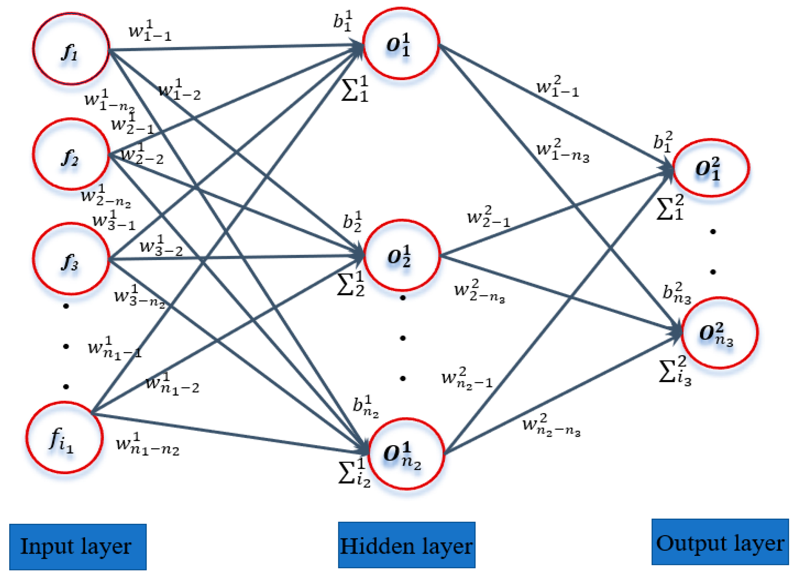
Figure 1. Architecture for artificial neural networks.

Figure 2. Chuong Duong bridge.

Figure 3. Detailed cross section of Chuong Duong bridge.

Figure 4. Placement of measurement points on span 8 of Chuong Duong bridge (blue: reference point, red: moving points) and sensor installation position at truss node.

Figure 5. Dynamic response sensor in time/frequency domain.

Figure 6. Stabilization diagram in an interval from 1 - 8.5 Hz.

Figure 7. Modes shape of Chuong Duong bridge in the campains: (a) Mode 1: f = 1.79 [Hz] (1st vertical bending); (b) Mode 2: f = 2.25 [Hz] (1st lateral + torsion); (c) Mode 3: f = 3.57 [Hz] (2nd torsion); (d) Mode 4: f = 4.30 [Hz] (2nd vertical bending); (e) Mode 5: f = 4.60 [Hz] (lateral movement); (f) Mode 6: f = 5.03 [Hz] (2nd lateral bending); (g) Mode 7: f = 8.09 [Hz] (3rd vertical bending).

Figure 8. FEM of span 08 – Chuong Duong bridge

Figure 8. Two types of bearing are used in the span of 8 Chuong Duong Bridge: a. type 1; b. type 2.

Figure 10. Seven first mode shapes from simulation: (a) Mode 1: f = 1.83 [Hz] (1st vertical bending); (b) Mode 2: f = 2.34 [Hz] (1st lateral + torsion); (c) Mode 3: f = 3.45 [Hz] (2nd torsion); (d) Mode 4: f = 4.06 [Hz] (2nd vertical bending); (e) Mode 5: f = 4.52 [Hz] (lateral movement); (f) Mode 6: f = 5.16 [Hz] (2nd lateral bending); (g) Mode 7: f = 8.39 [Hz] (3rd vertical bending).

Figure 9. MAC values: (a) before model updating; (b) after updating.

Figure 10. Frequency differences before and after updating

Figure 11. Architecture of ANN used in the research.

Figure 12. Regression values of ANN in case single damage.

Figure 13. Error histogram of ANN in case single damage.

Figure 14. Tolerance of network in case single damage.

Figure 15. Regression values of ANN in case 2 damages elements.

Figure 16. Error histogram of ANN in case 2 damages elements.

Figure 17. Tolerance of network of ANN in case 2 damages elements.

Figure 18. (a) Collision and damage at a truss rod; (b) Experiment to determine the natural frequency of the bridge.

Table 1. Frequency values of the 7 identified modes.

No	Frequencies [Hz]	Damping ratios [%]	Modal phase collinearity	Mode type
1	1.79	1.50	0.999	First vertical bending
2	2.25	1.06	0.998	First lateral + torsion
3	3.57	0.77	0.999	Second torsion
4	4.30	1.21	0.999	Second vertical bending
5	4.60	0.40	0.996	lateral movement
6	5.03	1.50	0.998	Second lateral bending
7	8.09	1.06	0.997	Third vertical bending

Table 3. Natural frequency and mode shapes of numerical model.

Mode	f-simulation (Hz)	f-measurement (Hz)	Error^*(%)	MAC	Type
1	1.83	1.79	2.23	0.87	1st vertical bending
2	2.34	2.25	4	0.85	1st lateral + torsion
3	3.45	3.57	3.36	0.86	2nd torsion
4	4.06	4.30	5.58	0.69	2nd vertical bending
5	4.52	4.60	1.74	0.83	lateral movement
6	5.16	5.03	2.58	0.72	2nd lateral bending
7	8.39	8.09	3.71	0.69	3rd vertical bending

(*) Error = |fsimulation – fmeasurement| × 100/fmeasurement.

Table 4. shows the range of variation for the uncertain parameters.

No	Uncertain parameters	Initial value	Upper bound	Lower bound
1	Young’s modulus - Steel E_s (GPa)	200	210	190
2	Weight density - Steel ρ_s (kg/m3)	7850	8000	7800
3	Masses of non-structural - m_b (kg/m)	3000	3000	5000

Table 5. Updated parameters.

No	Uncertain parameters	Initial value	Updated value
1	Young’s modulus - Steel E_s (GPa)	200	205.54
2	Weight density - Steel ρ_s (kg/m3)	7850	7956.5
3	Masses of non-structural - m_b (kg/m)	3000	3600

Table 6. Summary of natural frequency and mode shapes of the plate structure after updated.

Mode	f-simulation(Hz)	f-measurement (Hz)	Error^*(%)	MAC	Type
1	1.79	1.79	0.00↓	0.99↑	1st vertical bending
2	2.24	2.25	0.44↓	0.95↑	1st lateral + torsion
3	3.58	3.57	0.28↓	0.96↑	2nd torsion
4	4.33	4.30	0.69↓	0.94↑	2nd vertical bending
5	4.61	4.60	0.21↓	0.94↑	lateral movement
6	5.05	5.03	0.39↓	0.94↑	2nd lateral bending
7	8.15	8.09	0.74↓	0.94↑	3rd vertical bending

(*) Error = |fsimulation – fmeasurement| × 100/fmeasurement.

Disclaimer/Publisher’s Note: The statements, opinions and data contained in all publications are solely those of the individual author(s) and contributor(s) and not of MDPI and/or the editor(s). MDPI and/or the editor(s) disclaim responsibility for any injury to people or property resulting from any ideas, methods, instructions or products referred to in the content.

© 2024 by the authors. Licensee MDPI, Basel, Switzerland. This article is an open access article distributed under the terms and conditions of the Creative Commons Attribution (CC BY) license (https://creativecommons.org/licenses/by/4.0/).

Copyright: This open access article is published under a Creative Commons CC BY 4.0 license, which permit the free download, distribution, and reuse, provided that the author and preprint are cited in any reuse.

MDPI Initiatives

Important Links

Choose an area of interest and we will send you notifications of new preprints at your preferred frequency.

Disclaimer

Structural Assessment Based on Vibration Measurement Test Combined With an Artificial Neural Network for the Steel Truss Bridge

Abstract

1. Introduction

2. Theoretical Approach

2.1. Using Dynamic Features to Detect Damage

2.2. Artificial Neural Network

3. Case Study

3.1. Chuongduong Bridge Introduction

3.2. On-Site Measurement Campaign before Damage

3.3. FEM Creation and Updating

3.4. Generate Data and Train the ANN Model

3.5. The Service of the Trained ANN Model in Actual

4. Conclusions

Author Contributions

Acknowledgments

Conflicts of Interest

References

MDPI Initiatives

Important Links

Subscribe