Body Composition Estimation in Breeding Ewes Using Live Weight and Body Parameters Utilizing Image Analysis

Farmers are continually looking for new reliable, objective and non-invasive methods for evaluation of ewe condition. Live weight (LW) and body condition score (BCS) are used by farmers as a basis to determine the condition of the animal. Body composition is an important aspect of monitoring animal condition. The body composition is the amount of fat, lean and bone; knowing the amount of each is important because the information can be used for better strategic management interventions. Experiments were conducted to establish the relationship between body composition and body parameters, at key life’s stages (weaning and pre-mating), using measurements automatically determined by an image processing ap-plication at Lincoln University sheep farm for 88 Coopworth ewes. Computerized Tomography technology was used to develop relationship with body parameters and a subset was used to validate the predicted model. Multivariate linear regression (MLR), artificial neural network (ANNs) and regression tree (RT) statistical analysis methods were evaluated to determine their efficacy to predict body fat, lean and bone. The results showed a correlation between fat, lean and bone determined by CT and the fat, lean, bone weight estimated by live weight and body parameters calculated using the image processing application with R2 values of 0.90 for fat, 0.72 for lean and 0.50 for bone using ANNs statistical model. From these results, farmers can utilize accurate measures of fat which will enhance nutritional and management practices.

Keywords:

Subject: Biology and Life Sciences - Animal Science, Veterinary Science and Zoology

1. Introduction

Monitoring and improving individual animal performance is one mechanism to lift economic returns for sheep farming operations [1]. Body Condition Score (BCS) is a quick and easy way to evaluate ewe condition by hand based on the amount of fat on the lumbar region using a rating value between one and five; one represents poor and five represents obese [2]. A BCS between 2.5 and 3.5 means ewes are in good condition [3]. It is useful to check BCS before mating and during pre-lambing, as changes in body condition or amount of fat affect ovulation rates and lambing percentages: the ovulation rate peaked at a BCS of 3.0 [4]. BCS can provide an indication of percentage fat by well-trained evaluators, however, it is a subjective measure [5].

The relationship between BCS and LW varies based on age, physiological status and breed for ewes within the same flock [5]. In Merino ewes, LW could change by an average of 9.2 kg if the BCS changes by one unit but could be more or less for other breeds [6]. LW as an indicator of animal condition has limitations; such as gut fill and length of fleece [7]. In order for live weight to be used as an indicator, physical factors such as wool, and size would need to be taken into account [8]. Wool can vary between sheep breeds, e.g. wool length when shorn once during the year is 125-175 mm for Romney sheep but 65-100 mm for Merino sheep, Coopworth ewes fleeces weigh about 5 kg; staple length is in the range of 200–230 mm [9]. BCS is useful for farmers but has limitations and needs to be improved given the subjective nature of it. Due to repeatability between farmers in measuring BCS for the same ewe has significant differences which can limit the effectiveness and use of this technique [3]. Sheep farmers currently rely on LW and BCS to evaluate condition of ewes. One of the limitations of BCS is that, it is dependent on the specific person undertaking the BCS. Termatzidou et al. mentioned that a ewe that might be considered by a lowlands flock-master to be in only moderate condition (condition 2) could be judged as very good (condition 3.5) by someone accustomed to handling hill stock [10]. The study by Termatzidou et al. concluded that BCS had high variability between assessors for evaluating ewes condition and the development of a new scale is required to provide a more accurate estimation of percentage of fat for ewes. In the study, BCS was evaluated by assessors and fat was measured by ultrasound at two times (fattening and fasting) from four different breeds; Chios (n=80), Lacaune (n=70), Frizarta (n=75), Assaf (n=70). The result showed a weak to moderate correlation between BCS with fat, with a different fat among ewes at the same BCS with R²=0.69 for Chios, R²=0.38 for Lacaune, R²=0.72 for Frizarta and R²=0.01 for Assaf. In summary, BCS is an easy and quick on-farm method that describes the fatness of ewes. It helps farmers to get an indication of the amount of fat but does not provide an accurate estimation. In addition to accuracy/repeatability and small range score issues, thus the development of a new more objective body condition scale to assess animals is essential. The outcome of the study strongly indicates the need for the development of a new and more objective body condition scale to assess animals [10].

1.1. Body Composition

Body composition is an indicator of animal health status. Body composition is the amount of fat, lean and bone; knowing the amount of each is important because the information can be used for better farm strategic management interventions [11]. Prediction of fat, lean and bone amounts are desirable but the prediction of fat amount is more important than lean and bone, because fat is the source of stored energy that ewes rely on during pregnancy, lambing and weaning [12].

Four measurement points are routinely used throughout the production cycle by farmers to monitor the condition of ewes and the flock as a whole. In southern hemisphere, these are pre-mating (in late March or early April); pregnancy (90 days post-conception/first week of July); pre-lambing (two weeks before lambing/last week of August) and weaning (mid-December). Ideally ewes are monitored at each of these times, however, it is particularly important to check the ewe’s condition at weaning and pre-mating to ensure the ewe’s condition recovers after weaning as ewes must be in optimal condition at pre-mating [13]. These are particularly crucial times in a ewe’s life cycle to make sure it is ready for mating, ensuring ewe and lamb survival in the next lambing and the best performance of the animal during weaning [13].

It is advantageous for farmers to gather more information on body composition enabling them to perform the right interventions to maintain a healthy flock. The time between weaning and pre-mating is crucial as ewes lose more body condition in early lactation but compensate for these losses after weaning. There are numerous factors that effect this recovery such as age, nutrition [14], rearing, sex of lamb, random additive genetic effect [15] and environmental effects that cause health issues such as parasitic infections [16]. After weaning, farmers must be prepared to treat gastrointestinal parasites and selenium deficiency. The body composition profile of ewes between gestation and pre-mating indicates animals' reproductive performance, which can be utilized when making management decisions on-farm to improve productivity [17].

Some farmers use medical methods such as computerized tomography (CT) to accurately measure body composition for high valued rams. CT is an imaging technique that uses low-dose X-rays to produce images of body cross-sections and these detailed images provide an accurate estimation of body composition [18]. Due to the time, cost and nature of the processes, medical methods are typically only used with high-value animals such as breeding rams. The accuracy of CT compared with dissection for determining body composition achieved high R² values of 0.98 for fat, 0.92 for lean and 0.83 for bone. The accuracy of CT to measure body composition can be impacted by human error as it is manually measured by the CT operator [19]. CT scanning is time-consuming, require licensed staff to do scanning and require animal to be anaesthetized before scanning. Furthermore, body radiation exposure while scanning may affect the sheep, as they usually experience some discomfort while lying down on the CT scanners.

1.2. Body Parameters

Body parameters have been used to evaluate the characteristics of yaks and ewes to predict body size and LW [20]. Body parameters of diagonal length (angle), height and body side area were used to estimate yaks’ body weight using image analysis in summer for 39 yaks, in winter for 52 yaks and in spring for 55 yaks [21]. The result showed a correlation with R² of 0.90 for angle length, 0.94 for height, 0.74 for side area in summer, 0.83 for angle length, 0.85 for height, 0.91 for side area in winter and 0.70 for angle length, 0.78 for height, 0.68 for side area in spring respectively between the weight measured by the scale and the weight predicted by the body parameters. A slightly higher correlation using body dimensions of front height, back height-hip cross, body length-shoulder to buttocks, depth and chest circumference were found to estimate body weight using image processing for 25 yaks [22]. The yaks were off-feed for 12 hours prior to imaging to ensure the animals were in a fasting state. Body parameters were measured three times, the average value was taken. The front height, back height and depth were measured by a measuring stick while body length and the circumference were measured by a tape. The results showed a correlation between live weight determined by the electronic scale and the weight calculated by body parameters utilized by the image processing with R² of 0.92 of front height, 0.88 of body length, 0.95 of depth and 0.91 of circumference using linear regression, respectively with maximum error detection of 17.6 kg and minimum error detection 11.1 kg. Ultrasound scanning, visual camera measurements and carcass data after slaughtering were correlated and used in beef cattle [23]. Multiple linear regression was used for the prediction of fat and lean using ultrasound measurements. The correlation of the three methods ranged from 0.79 to 0.82 for ultrasound data, 0.68 to 0.95 for visual camera measurements, and 0.57 to 0.87 for carcass data of back fat and Longissimus muscle area, respectively. The ultrasound data were collected 24 hours before slaughtering, carcasses were chilled for 48 hours after slaughtering, camera measurements were collected by plant personnel and carcass data were collected by well-trained evaluators. Data included were twelfth and thirteenth rib back fat thickness (cBF), twelfth and thirteenth rib LM area (cLMA) and degree of marbling. A study of sheep body fat and carcass composition prediction using ultrasound measurements and LW was published by Dias et al. [24]. This study obtained fat thickness at the lumbar (U_LUMB, fat thickness measurement between the third and fourth lumbar vertebra) and sternal (U_STER, fat thickness measurement on third sternebra) region by using ultrasound. The method to estimate total body fat on lamb found a relationship between independent variables LW, sternum fat depth multiplied by LW, lumbar subcutaneous fat depth multiplied by sternum fat depth, sternum fat depth, lumbar subcutaneous fat depth and dependent variable the total body fat resulting in predicted multiple linear regression models with R² between 0.79 and 0.95. In addition to fat, a relationship was found between the muscle determined after slaughtering and achieved an R² of 0.96 using independent variables LW and sternum fat depth obtained by ultrasound measurement and had a residual standard error of 600 g [24].

Ultrasound and CT scanning are used in the New Zealand sheep industry to estimate the body composition of live animals. Whilst full-body CT images can be generated, the cost of such an approach is prohibitive from a commercial perspective. However, an alternative to using CT scanning to predict internal fat reserves would be to develop predictions based on ultrasound measures of internal adipose deposits by Morales-Martinez et al. [25] in Pelibuey sheep. By measuring kidney adipose thickness using ultrasonography, they were able to predict internal adipose reserves relative to dissected internal adipose reserves with an R²= 0.77. Generally, four major fat deposits are recognized in animal carcasses: subcutaneous (under the skin), internal organ associated (surrounding the kidneys and other internal organs), intermuscular (between muscles) and intramuscular (IMF, within the muscle), the latter having the greatest association with meat-eating quality. A correlation was found between body composition weights measured from the full set of CT images and body composition weight measured from the sub-set of CT images (six images instead of 32 images) of 50 ewes. The idea was to investigate if a sub-set of CT slices could provide the same accuracy as full CT, which would save time and cost. The CT data were obtained from the forequarter (fifth thoracic vertebrae and seventh cervical vertebrae), the loin (sixth lumbar vertebrae), the rack (thirteenth thoracic vertebrae) and the hind-leg (second caudal vertebrae and third sacral vertebrae). The result supported using a sub-set instead of a full CT scan, with a correlation of 0.92 for sub-cutaneous adipose and 0.25 for bone [26].

Body parameters can be measured by hand, measuring stick, tape measure and image analysis where sheep must stand in a place with correct posture (the sheep’s body is straight and the head is not turned to the left or the right). Body parameters such as body length, rump height, withers height, back height, chest girth, chest depth and chest width are used to estimate LW and frame size [27]. Body parameters of withers height, body length, chest girth, paunch circumference, face length, length between ears, ear length, fat tail width and tail length were used to predict the LW of sheep collected from 757 (247 male and 510 female) indigenous Harnai sheep of Pakistan. The body weight of sheep was measured using a digital scale while other body parameters were measured with a measuring tape. The result showed a relationship between the LW determined by scale and the weight estimated by the body parameters, with an R² value of 0.92 using Penalized regression (keeping all predictor variables in the model, but constraining the coefficients by shrinking them toward zero) [28]. Research by Sabbioni et al. [29] used more body measurements of height at withers (HW), chest circumference (CHC), body length (BL), height at croup (HCR), chest width (CHW), chest depth (CHD) and croup width (CRW) to predict the LW of Cornigliese sheep. This research measured the body parameters using a flexible tape measure. The result showed a high R² of 0.96 and root mean square error (RMSE) of 4.87, confirming that the LW of this breed can be predicted using body measurement.

Zhang et al. [30] investigated and proposed a method to estimate body dimensions using body parameters measurements based. Top and side images were captured of each animal with wool using three cameras measure the body parameters automatically. The method used a blue background and underground to distinguish the sheep's body from the surroundings. The study concluded that image processing analysis can be used on-farm to measure sheep dimensions in an automatic non-contact measuring method. This method does not cause stress to animals and farmers and it reduces the likelihood of anthropozoonosis (infectious diseases that are naturally transmitted from humans to animals) [30]. The result showed for different images of the same ewe different body parameters measurements were found. The greatest difference was for the body length, which ranged between -4.5 to 2.2 cm and the smallest difference was for rump width, which ranged between -1.2 to 0.9 cm.

The feasibility of using image processing to estimate the LW of sheep was investigated, and the research indicated that image analysis using body parameters can be used as a reliable guide for estimating the LW and body size of sheep [31]. Body parameters of heart depth, height at wither, chest width, heart girth and rump width were used to estimate sheep body weight. The highest R² of 0.75 was found using the heart girth to estimate the body weight [32]. Body parameters of body length, rump height, withers height, back height, chest girth, chest depth and chest width were used to predict the body weight of 215 sheep. The sheep were divided into five age groups between 2-6 years in mating time with the highest R² of 0.79 found in the LW estimation using body length. The LW was obtained by a digital scale with 50 g sensitivity and body parameters were measured by tape measure [27]. In addition to LW, another study indicated that the image processing technique can be used for estimating new-born lamb score size, suggesting that the image processing method is a more accurate tool than the human appraisal method [33]. The human appraisesal method was used to evaluate the new-born body size by a trained evaluator, with allocation of scores as follows: score 1 for small body size animal, score 3 for medium size and score 5 for big size. The metric method, based on determining the body parameters by tape measure was used as a reference against the body parameters determined by image analysis [34]. The image processing technique used side images of lambs in the RGB scale, greyscale images and then images without limbs, trunk, head and neck. All images were converted from colour images to greyscale using MATLAB 7.8.0 software. Considering the fixed imaging distance and equal size of all input images, the area of the lateral side of each lamb was estimated by counting the number of white pixels in the binary image. The result shows a correlation coefficient with an R2 of 0.48 between lamb body size which was measured using the metric method (based on determining the body parameters by tape measure was used as a reference against the body parameters determined by image analysis) and values obtained by the appraisal method. A higher correlation coefficient (R² of 0.88) was found between the metric method and the image processing. This means image processing techniques could be used on-farm as they achieved more accurate results than the human appraisal [33].

A study used body parameters to estimate fat of pigs with an R² value of 0.69 using the body rump width parameter determined from a top image view [35]. Parameters of side image view such as body angle length, height and depth were found to be highly correlated for predicting of body size [36] and LW [37]. The relationship between body parameters and carcass characteristics of hair lambs of Pelibuey and Katahdin breeds was studied [38]. This study used 66 hair lambs; 30 were single lambing and 36 were double lambing. Body parameters of height at withers, rib depth, body diagonal length, body length, pelvic girdle length, rump depth, rump height, pin bone width, hook bone width, abdomen width, girth circumference and abdomen circumference were taken using tape measure 24 hours prior to slaughter. A fasting procedure for 20 hours was followed before slaughtering in order to record shrunk body weight of lambs. Hot carcasses were weighed after 24 cold carcasses were split by the dorsal midline into two halves and reweighed. The Left halves were dissected into muscle, fat, bone tissues and the weights of the tissues were doubled to reflect the total carcass weight. The weight of viscera, organs, skin, offal, head, feet, tail and blood was also recorded. Regression equations were used to find relationships between body parameters and carcass characteristics. The result showed an equation to estimate carcass weight from shrunk body weight, pelvic girdle length and abdomen circumference with R² of 0.94. Total soft tissue (fat and muscle) weight was predicted using shrunk body weight, rump depth, abdomen circumference and hook bone width with R² of 0.91. Bone weight was predicted shrunk body weight, rib depth and girth circumference with R² of 0.86 [38].

A summary of studies showing the relationships between independent and dependent variables is shown in Table 1. Body composition estimation using body parameters has not been widely applied to live animals. The focus has been on predicting animals’ weight and size. Therefore, this paper proposes to investigate a new method using body parameters determined by image analysis coupled with a weight measurement to estimate the body composition of Coopworth ewes. Body parameters obtained through image processing have been used on live sheep to estimate LW, and body size but have not been used to estimate body composition. Determing body composition is important as it provides accurate measure for amount of fat, muscle and bone, which help farmers to eveluate animal condition during production cycle. For example, if the amount of fat decreases at pre-mating nutritional intake is required.

Body parameters were used to estimate the LW of yaks and sheep and fat weight for pigs. The study by Iqbal et al. [28] used more body parameters than the other studies to estimate the body weight of sheep (withers height, body length, chest girth, paunch circumference, face length, the length between ears, ear length, fat tail width and tail length). The highest R² value for sheep body weight estimation reached 0.99 for the study done by Zhang et al. [39] using body parameters of withers height, back height, rump height, body length, chest depth, chest width, abdominal width and rump width. Different linear and non-linear statistical methods were used, but the majority of studies used multiple linear regression.

Multiple linear regression (MLR) was the main statistical method utilized to find the relationships between independent and dependent variables for the majority of studies. MLR is used to develop a statistical model between dependent and independent variables to estimate the LW, body size and carcass characteristics.

This research investigates the use of body parameters determined by image processing and LW to estimate body composition during ewe production cycle instead of using BCS (indicates fat only). Furtheremore, it explores MLR as well as two non-linear methods which is two-layer feed-forward Artificial Neural Networks (ANNs) utilizing Levenberg-Marquardt back-propagation algorithm; and Regression Tree (RT) machine learning.

Table 1. Summary of studies to predict body composition.

Authors - Year	Dependent variables	Independent variables (R²)	Statistical method
Yan et al. – 2019 [21]	LW of yaks measured by digital scale	Angle length (0.90), height (0.94), Side area (0.74)	Multiple linear regression
Zhang et al. – 2020 [22]	LW yaks measured by digital scale	Height (0.92), body length (0.88), body depth (0.95), circumference (0.91)	K-Nearest Neighbour
Ribeiro et al. – 2014 [23]	Back fat thickness and longissimus muscle area – Beef	Back fat thickness in cm and longissimus muscle area cm² (0.68 to 0.95)	Multiple linear regression
Dias et al. – 2020 [24]	Fat Lean	LW, sternum fat depth multiplied by LW, lumbar subcutaneous fat depth multiplied by sternum fat depth, sternum fat depth, lumbar subcutaneous fat depth and dependent variable the total body fat (0.68 to 0.95) LW and sternum fat depth (0.96)	Multiple linear regression
Morales-Martinez et al. – 2020 [25]	fat	measuring kidney adipose thickness (0.77)	Multiple linear regression
Johnson et al. – 2020 [26]	Internal fat	Forequarter, loin, rack and the hindleg (0.92)	Multiple linear regression
Yilmaz et al. – 2013 [27]	LW sheep measured by digital scale	Body length (0.79)	Multiple linear regression
Iqbal et al. – 2019 [28]	LW sheep measured by digital scale	Body weight, withers height, body length, chest girth, paunch circumference, face length, the length between ears, ear length, fat tail width, tail length (0.92)	Penalized regression
Sabbioni et al. – 2020 [29]	LW sheep measured by digital scale	Height at withers, chest circumference, body length, height at croup, chest width, chest depth and croup width (0.96)	Multiple linear regression
Topai and Macit – 2004 [32]	LW Sheep measured by digital scale	Heart girth (0.75)	Multiple linear regression
Doeschl et al. – 2004 [35]	fat weight Pigs measured by slaughtering and dissection	Rump width (0.69)	Multiple linear regression
Zhang et al., 2018 [36]	LW sheep measured by digital scale	Withers height, back height, rump height, body length, chest depth, chest width, abdominal width and rump width (0.99)	SMV
Abdelhady et al. – 2019 [37]	Live Weight Sheep measured by digital scale	Body breadth and Body length (0.98)	Multiple linear regression
Diaz et al. – 2020 [38]	Muscle&fat weight by slaughtering Bone weight by slaughtering	shrunk body weight, rump depth, abdomen circumference and hook bone width (0.91) shrunk body weight, rib depth and girth (0.86)	Multiple linear regression

2. Materials and Methods

2.1. Experimental approach

Body composition was determined using CT scanning. The LW and BCS of ewes were then recorded, as well as top and side visual images which were used to determine body parameters using image processing. Statistical analysis and modelling were then undertaken to determine which body measurements provide predictive power in predicting body composition. Factor analysis was used to check the correlation between the body parameters of the training data.

Data were collected at two time periods; at weaning where ewes have their lowest condition and at pre-mating where ewes were at their best condition. The data from the CT scan, LW and visual imaging were collected. The data at the weaning scan were collected from 88 ewes where the data at the pre-mating scan were collected from 74 ewes.

The body parameters were obtained from top and side view images using an image processing application built for this purpose. Image processing methods were used to calculate the body parameters. The LW and BCS were collected by a farm manager.

Before data collection, the body parameters were measured by tape measure and a custom-made ruler to find the tool with less error. After experimentally verifying these tools, it was found that the custom-made ruler was more accurate, quicker and less stress on the sheep when measuring the body parameters than tape measure. In the weaning and the pre-mating scan, physical measurements were captured to estimate error of the image analysis method.

Three top images were taken using GoPro 7 camera (12 Megapixel) mounted orthogonally with a height of 2350 mm from the ground. This height was sufficient to produce a non-distorted image. The goal behind taking three images was to get a picture with ewes standing straight. The side camera was a Canon DSLR 750D and was used to capture up to three visual side view images with 6000 mm between the center of the ewe and the camera and 760 mm height between the ground and the camera. The camera had a 24.2 Megapixel CMOS sensor, a DiG!C 6 image processor and EF-S 18-135mm f/3.5-5.6 IS STM lens. While taking the top and side images, two small whiteboards were used to report the animal ID, which was used later during the analysis to identify the animal. A 400 mm ruler was placed on the animal’s body and later used in the analysis of the images to calculate the scale of 400 mm for each image and define the actual dimensions Figure 1.

2.2. Data collection

2.2.1. CT scans

Ewes were CT scanned at the Lincoln University CT lab, followed by LW and BCS determined by a farm manager (has 20+ years of experience). Finally, top and side images were captured.

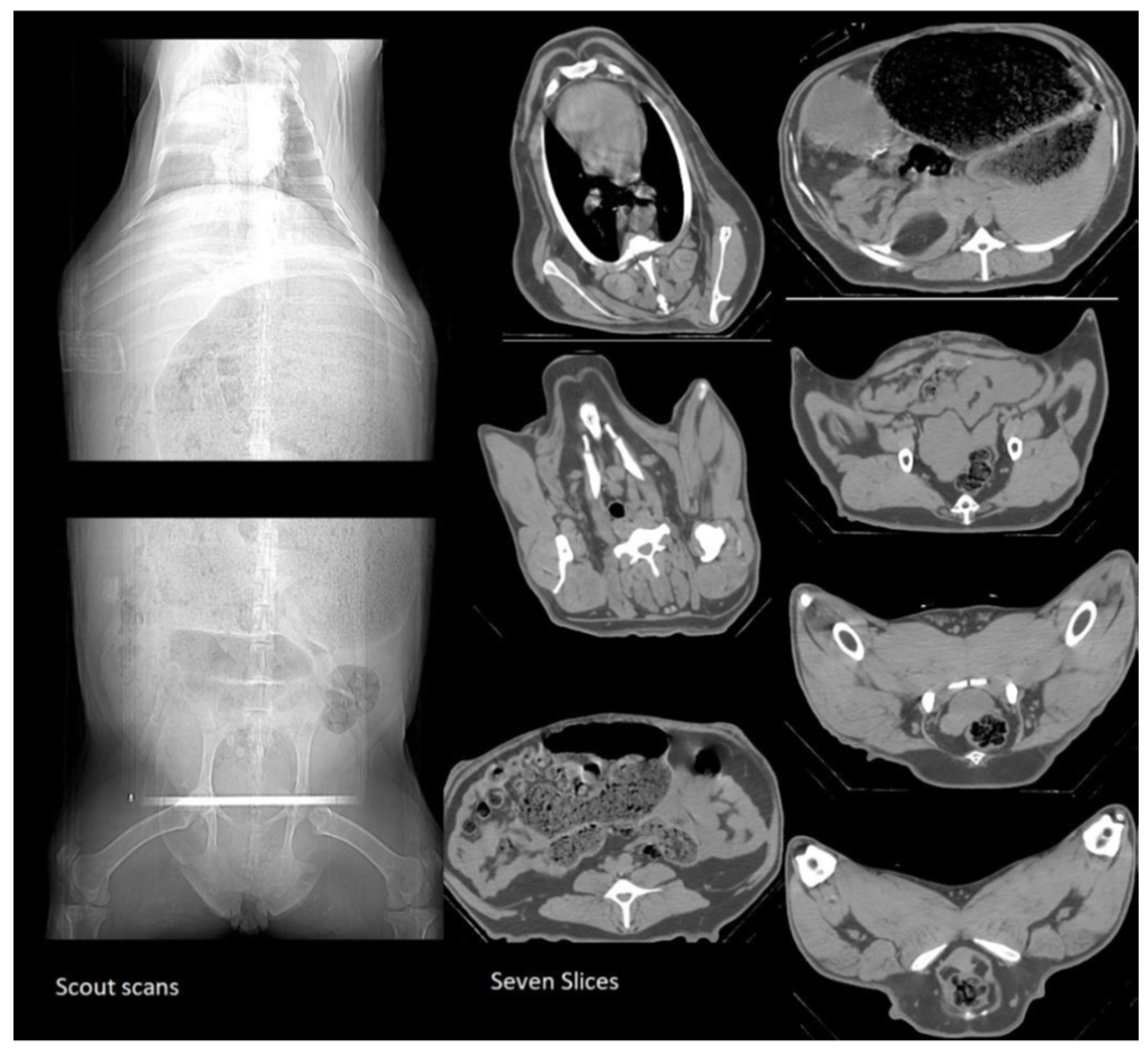
The data were collected in December 2020 during the weaning stage of the production cycle and in March 2021 for the pre-mating scan. The CT slice measurements were measured manually by the CT operator using STAR 6.15 software. The amount of fat, lean and bone for each slice based on the colour (fat in dark grey areas, lean in light grey areas, bone in white and in air black areas) by drawing around these areas within the CT software. Lincoln University SOP 83 and Animal Ethical Committee (AEC) #642 approval were followed for the capturing of CT data, LW and manually measuring body parameters and BCS.

A two-scan approach was adopted to determine ewe body composition using a CT750 HD machine and STAR 6.15 software. The animals were brought indoors and fasted with the water removed for 12 hours before scanning. The next day, at 9 am, the animals were moved to the CT lab for CT scanning. The ewes were tranquillized with acezine 10mg administered intramuscularly at 0.1 ml/per 10 kg (e.g., a 60 kg ewe was given 0.6 mL, and a 70 kg ewe was given 0.7 mL, and so on) to relax their muscles and keep stress to a minimum. This dosage scheme was prepared in the same syringe and provided 20 to 30 minutes of adequate sedation and analgesia for ewes. After five minutes and once sedated, the ewe was loaded into a wooden CT scanning stretcher in the sternal recumbence position (on its back).

Two scout scans were taken: one from the top half of the body and another from the bottom half. The first scout scan captured three slices of the ribs. Slice 1 was taken at the first rib, slice 2 at the fifth rib and slice 3 at the last rib. The second scout scan captured four slices: one at the second to the last vertebra in the spine; the second slice at the fifth rib in the middle of the pelvis; the third slice at the end of the pelvis; and the last slice was taken at the ischium Figure 2. Once the scanning procedure was completed, the wooden stretcher was carried out and the ewe was released to the recovery room. The ewe was placed in the sternal recumbence recovery position and ensured that it was kept warm.

2.2.2. Body measurements

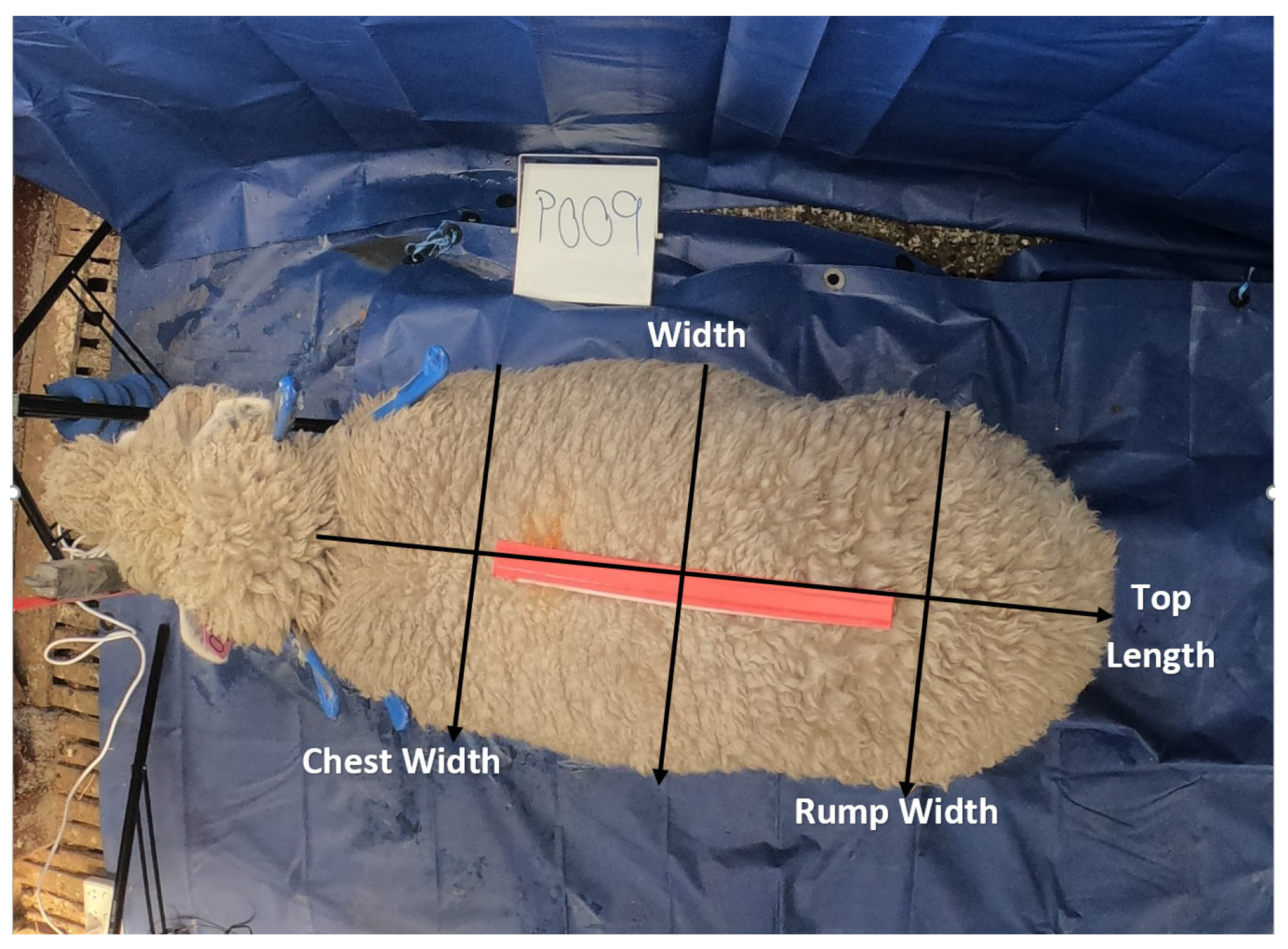
Using Prattley 3-way weigh crate scale, the ewes' LW was measured and the BCS was evaluated by the farm manager. The ewes were secured in a neck brace then top and side images were taken. The neck brace stopped the ewes from moving and helped in having standard standing position. The aim was to keep the ewes standing in comfort without disturbance when capturing the images. The top body parameters were chest width, width, rump width, top length and top area (top body area without head) as shown in Figure 3.

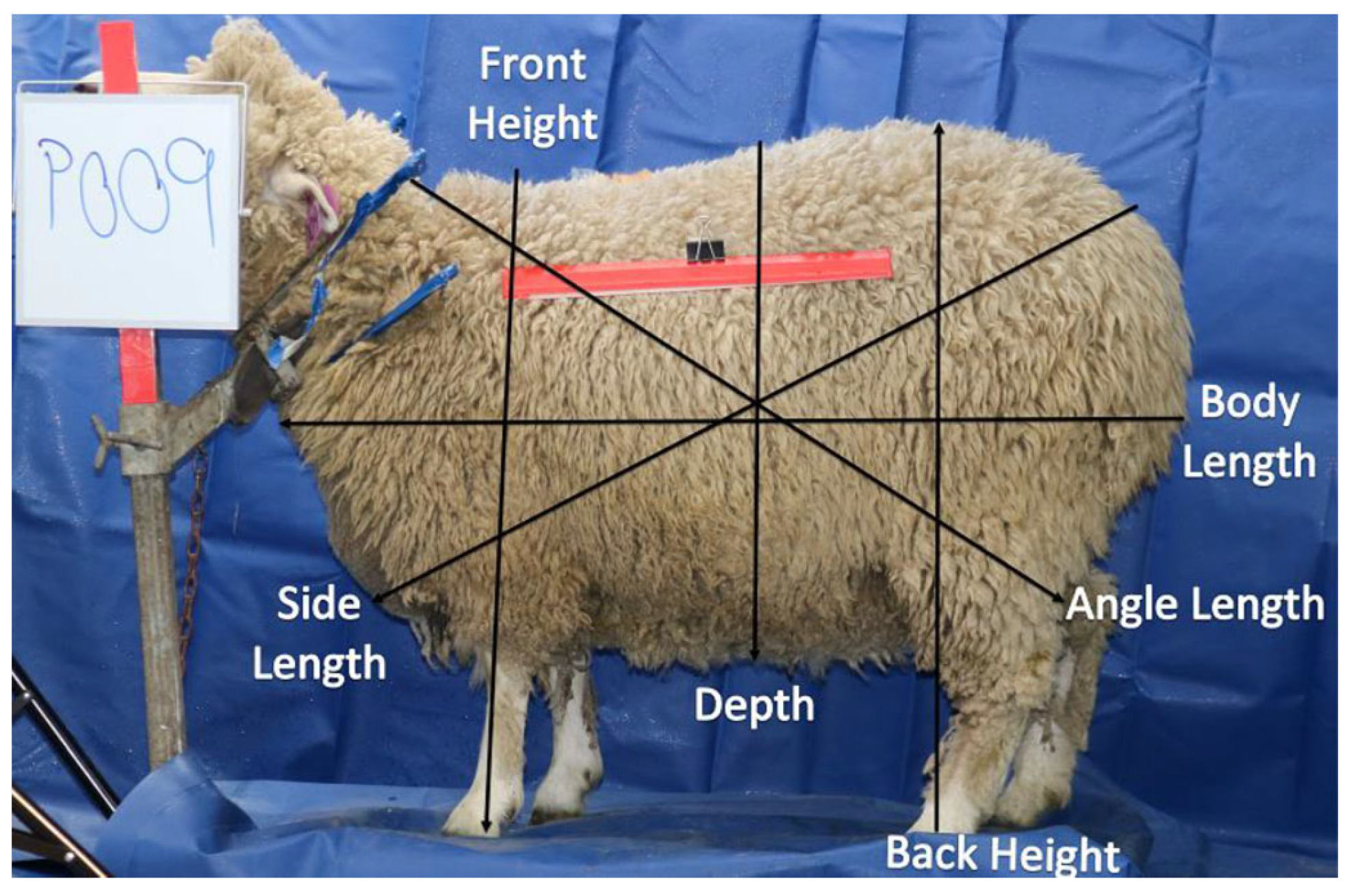
The side body parameters were body length from brisket to the top point of the leg, side length from the rump dock to the forearm, angle length from the neck to the top point of the hock, the height from the lowest point of the front hoof to the top shoulder, depth from the top rack to the lowest point of the belly and the side area (side body area without head and legs) Figure 4. Body parameters of width, top length, front height, body length, angle length, depth and side length, chest width, rump width, back height top and side areas were calculated by image processing application at weaning and pre-mating scans.

2.2.3. Visual image capture

Three top images were taken using a GoPro 7 camera (12 Megapixel) mounted orthogonally with a height of 2350 mm from the ground. This height was sufficient to produce a non-distorted image. The goal behind taking three images was to have backup images for each ewe in case ewe was moved while taking first image.

The side camera was a Canon DSLR 750D and was used to capture up to three side view images with 6000 mm between the center of the ewe and the side camera and 760 mm between the ground and the top camera. The camera had a 24.2 Megapixel CMOS sensor, a DiG!C 6 image processor and EF-S 18-135mm f/3.5-5.6 IS STM lens. While taking the top and side images, two small whiteboards were used to report the animal ID, which was used later during the analysis to identify the animal. A 400 mm ruler was placed on the animal’s body and later used in the analysis of the images to calculate the scale of 400 mm for each image and define the actual dimensions.

2.3. Wool test

This test aimed to quantify the impact of wool length on the body parameters of five ewes and find wool adjustment amount. Five ewes were selected for the wool test, where their wool was shorn and body parameters were taken again. The body parameter results of the five animals showed the length of wool was 120 mm (the length of a strand of wool). The results show how shearing the wool affected the body parameters. The measurements were less for all body parameters for all animals, which was expected as the wool length was 120 mm. The difference between the five ewes before and after shearing the wool was calculated and the average was then calculated. An analysis was done to determine the wool correction factor for the pre-mating data as the average wool length was 60 mm. This average was divided by two and the constant found in millimeters. The average adjustment amount was found to be 24 mm for height, 29.5 mm for the depth, 30 mm for angle length, 46 mm for body length, 12 mm for top length, 45 mm for width, 700 mm² for side area and 610 mm² for top area. These constants were used to adjust all pre-mating data. After the adjustment, all parameters decreased slightly and LW decreased by 1200g as average wool weight is 5000 g for Coopworth ewes when wool length is 230 mm where in pre-mating scan wool length was 60 mm [9].

2.4. Analysis

After data collection, the top and side images underwent an image processing application and the dimensions were calculated. An application was built for this purpose to determine body dimensions such as body length, depth, height and width. This application was developed using image processing functions from OpenCV integrated and supported the development of the image application.

Models were developed using three main statistical methods: multiple linear regression; a two-layer feed-forward artificial neural network utilizing Levenberg-Marquardt back-propagation algorithm; and regression tree machine learning.

The statistical methods were applied to all data, three statistical models were compared to find the best model in terms of R² value and error percentage. In the two weaning and pre-mating experiments, data from 88 ewes was used; 74 ewes were scanned in both experiments and 14 ewes were scanned only once. For the ewes that were scanned in both experiments, each animal has two records. The data from these two experiments were combined, yielding 162 records or observations to cover different body compositions during weaning and pre-mating, as the objective is to develop one model that can be used to predict future body composition at any stage in the production cycle. The data for MLR and regression tree were then divided into two groups: one had 138 observations (selected from all ewes on weaning and 50 ewes from pre-mating scans), which was called training data for body composition prediction and the second group of 24 records (taken from 34% of pre-mating scan data), which was called test data. For ANNs, the percentages and number of observations were 162 observations, which were divided into three groups: 70% for training (114 observations), 15% for validation (24 observations) and 15% for testing (24 observations). The test data have different LW, BCS and size at pre-mating. This data was used to test the predictive power of the first group-body composition prediction. The objective behind this combination was to get a prediction for each body composition item over weaning and pre-mating times. All models used a single dependent variable (fat, lean, bone) and one or more independent variables.

3. Results

3.1. Descriptive statistics

The descriptive statistics are presented for 138 records (training data) collected from 88 ewes in the weaning and pre-mating CT scans (74 ewes scanned in both experiments and 14 ewes scanned only once). The descriptive analysis shows the minimum, maximum, mean and standard deviation of all ewes in Table 2. The amount of fat had wider range compared with lean and bone. The minimum fat amount determined was 0.88 kg compared to a maximum of 17.64 kg, while the minimum bone amount determined was 2.03 kg and the maximum was 3.77 kg.

The ewe with the lowest fat of 0.88 kg had a BCS of 2.0 and the lowest LW of 54.0 kg, while the ewe with the highest fat of 17.65 kg had a BCS of 4.5 and the highest live weight of 88.5 kg. The above table also shows how the ewes had a wide range of body composition, LW and body parameters with the BCS, ranging from a 2.0 to 4.5.

3.2. Error estimation

A repeat test run was conducted on 12 ewes using the custom-made ruler randomly selected with different LWs and frame sizes before doing the weaning and the pre-mating scans. The purpose was to quantify the repeatability of measuring when physical measurements were repeated twice for the same animal at two separate times and therefore determine the uncertainty Table 3. The result showed that there were differences in measurements between the tap measure and the custom ruler. The results showed a mean absolute error of 1% when using the custom-made ruler.

3.3. Application accuracy

The accuracy of the application aimed to determine the differences of body parameters between image processing application calculation and manual measurements as described in method section. The average change in percentage between body parameters taken by the farm manager and calculated by the application are shown in Table 5. The result showed 4% average absolute differences for all body parameters during weaning and pre-mating.

3.4. Factor analysis

The objective of the factor analysis is to determine which of the independent variables can be used to develop equations and avoid multi-collinearity issues in the creation of the three statistical models. The principal component analysis extraction method was used and divided the independent variables into three groups. The collinearity check in Table 6. shows collinearity between independent variables based on three components where each component has variables that had high collinearity between them. The first component includes chest width, angle length, body length, side length, top length, width, rump width, top area and side area. The second component includes BCS and LW. The third component included height and back height.

Training data of 138 ewes at weaning and pre-mating were used to develop relationships between the data set consisting of three dependent variables - fat, lean, bone- and the 13 independent variables. The aim was to predict those three dependent variables based on independent variables utilizing three different statistical methods: multivariate linear regression, artificial neural networks and regression tree. Models with all variables (13 inputs: LW, chest width, angle length, body length, side length, front height, back height, depth, top length, width, rump width, top area and side area) were also examined to compare all results.

3.5. Fat

P-value, R² and MSE values were used to test quality of the models. All predictors have a significant P-value less than 0.05 for the models and independent variables, with the highest adjusted R² value and lowest RMSE value considered with no co-linearity. After testing all possible combinations of the independent variables' for the estimation of fat based on factor analysis Table 7. A relationship between the independent variables’ weight and chest width with the dependent variable fat. The final multivariate regression model estimated the fat with R²=0.79 and RMSE =1.34 with no co-linearity obtained.

The result showed an R² of 0.87 and RMSE=1.40 using a set of test data to test power of the fat prediction for 24 random ewes.

For ANNs, the predicted model accounts for fat with R²=0.88 and RMSE=1.17. This model has two inputs - weight and chest width - with one hidden layer and one output (fat) with no collinearity. However, all variables model was examined to show the possible maximum result and had R²=0.95 and RMSE=1.22 Table 8. The known amount of fat was tested and a relationship was found to validate the fat prediction model using the test data with an R² value of 0.94 and RMSE=1.01.

For the regression tree, different combinations between body parameters were analyzed and compared. The model with the highest R² value and lowest RMSE for the prediction of fat was using two variables: LW and chest width with R²=0.67 and RMSE=1.75. The model was validated and the result showed R²=0.72 and RMSE=1.42 for predicting fat.

3.6. Lean

The highest R² to estimate lean was found between LW and width model. The model is found to be statistically significant (p-values=<0.05). The model with the highest R² value and lowest RMSE was chosen; the final multivariate regression model with R²=0.52 and RMSE=1.03 with no co-linearity is obtained and equation is displayed in Table 9. The result for test data showed an R² value of 0.41 and RMSE=0.86 between the actual and predicted lean.

After testing all possible combinations between the independent variables, one model showed the highest R² value and the lowest RMSE using ANNs. The best predicted model accounted for lean with R²=0.77 and RMSE=1.26, with one hidden layer used and three inputs (LW, rump width, front height). Where the highest predicted model accounted for lean with R²=0.79 and RMSE=1.20 for training data and R² value of 0.72 and RMSE=1.03 for test data Table 10.

The regression tree model for prediction of lean from independent variables used LW, width and chest width. The results showed lean with R²=0.25 and RMSE=1.27 for training data and R²=0.21 and RMSE=1.19 for test data.

3.7. Bone

The highest R² was found for the relationship using all of the variables, but this relationship was rejected as it is against the factor analysis. The next highest R² value to estimate bone was found for the relationship between LW and width. This model found to be statistically significant (p-values=0.00) with R²=0.26 and RMSE=0.87 with no co-linearity is obtained in Table 11.

The result of test data showed an R² of 0.34 and RMSE=0.26 between CT bone and predicted bone. It was noticed that the bone had a very small variation between 2.03 kg and 3.77 kg, which could explain the low R² value as mentioned in descriptive statistics.

All possible combinations of the independent variables were compared according to the highest R² value and the lowest RMSE. The heights R² value of 0.75 with an RMSE of 2.40 to estimate bone found using all variables. However, one model has three inputs: LW and width, front height, one hidden layer. The predicted model accounts for bone with R²=0.72 and RMSE=1.11 Table 12.

Test data of 24 ewes used to test the power of the predicted model for estimating bone with an R² value of 0.50 and RMSE=1.21.

The model with LW, rump width and chest width was the model to estimate the amount of bone, with R²=0.05 and RMSE=0.30 using regression tree. The best model for bone estimation was tested using 24 ewes of test data. The result showed R²=0.03 and RMSE=0.70.

3.8. Summary of results

All statistical methods results were compared to test the predictive power of the training models on a test data set of 24 ewes at the same points of the breeding cycle Table 13.

In terms of training data, three statistical models to account for fat were constructed. The most successful model was the ANNs, since when R² values were compared (0.79 - MLR, 0.88 - ANNs, 0.67 - regression tree), ANNs performed better than the other models. RMSE=1.17, input variables were LW and chest width. Three models were compared for lean (0.52 - MLR, 0.77 - ANNs, 0.25 - regression tree). ANNs showed highest R² value than the others models. RMSE=1.26, variables are LW, rump width and front height. Three models values were compared for bone (0.26 - MLR, 0.75 - ANNs, 0.05 - regression tree), ANNs showed highest R² value than the other models. RMSE=2.40, input variables were LW, width and front height.

In terms of test data, ANNs models were produced to estimate dependent variables. The ANNs showed the highest results for test data over MLR and RT for fat with R²=0.90 with RMSE=1.01, lean R²=0.72 with RMSE=1.03 and bone R²=0.71 with RMSE=1.21.

In summary, ANNs models are the best in terms of highest R² values and lowest RMSE for prediction of fat, lean and bone than MLR and RT. ANNs matrixes were produced to estimate body composition using input variables.

The result of fat estimation for the test data between the ANNs, MLR and RT along with BCS results are shown in Table 14. The maximum difference for the MLR compared with CT fat was 3.1 kg and there was a minimum difference of 0.002 kg. Where for ANNs, has 2.69 kg maximum difference and 0.034 kg minimum difference. The RT has a maximum difference of 8.34 kg and a minimum difference of 0.59 kg.

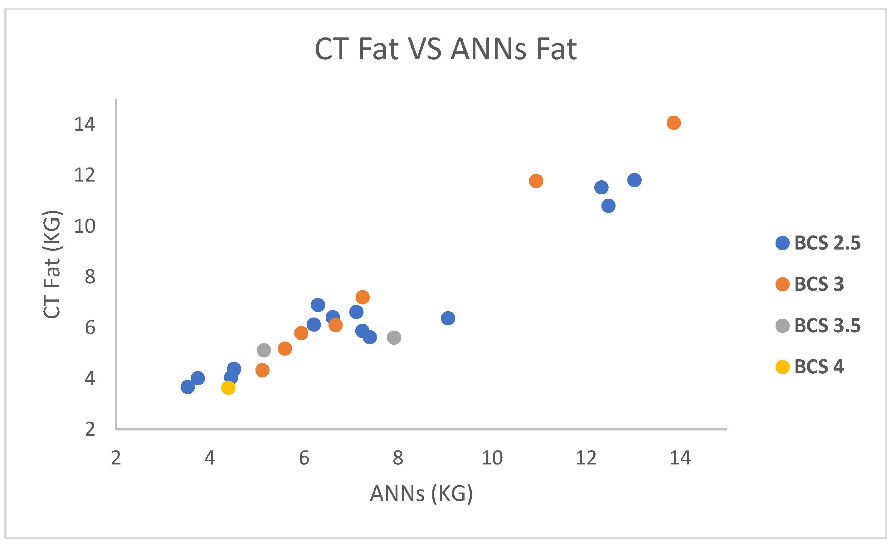
The BCS result showed a range of fat estimation between 3.52-13.03 kg for condition 2.5, 5.11-13.86 kg for score 3.0. Two ewes had a fat amount of 5.14 kg and 7.91 kg with condition 3.5, another ewe had a fat amount of 4.39 kg with a condition score of 4.0. The CT fat and ANNs fat results based on BCS are shown in Figure 5.

4. Discussion

An objective on-farm method to predict the body composition of ewes during their production life cycle was established. This helps to evaluate the status of energy reserves and provides the required nutritional intake for the ewes to gain what was lost during lactation (when ewes are at their lowest condition) until they return to their best condition at pre-mating time [40]. The new method requires less effort, time and does not need technical expertise and tranquillization of sheep with Acezine like the CT method [19]. CT method has high R² values of 0.98 for fat, 0.92 for lean and 0.83 for bone where the new method showed less R² values of 0.90 for fat, 0.72 for lean and 0.50 for bone.

Body fat is predicted on-farm by subjective methods like BCS [10]. As discussed in the literature review, BCS has a weak to moderate correlation with the fat of ewes and a difference of up to 0.5 BCS unit can exist among ewes at the same fat deposits and muscle mass. The study by Termatzidou et al. [10] concluded that the development of a new BCS scale is required to provide a more accurate estimation of the fat of ewes, as no one to develop a new scale. BCS can provide a good indication for fat percentage as stated by [5]. In contrast, the result of this research showed that BCS of ewes for the data set ranged between 2.0 and 4.5. Chest width ranged from 220.30 to 360.24 mm, the minimum amount of fat was 0.88 kg and the maximum 17.65 kg. The result showed that many ewes had the same BCS which provided a rough indication of ewe condition, but a wide range of chest width and fat measurements, confirming that BCS is not just subjective but also inaccurate to evaluate fat. For example, one ewe had 5.2 kg of fat, a BCS of 3.0 and chest width of 252 mm at weaning, then 7.1 kg fat, 3.0 BCS and chest width of 327.6 mm at pre-mating. This shows that fat and chest width increased over time, but BCS remained the same.

The results of training data showed a range of fat for BCS 2.0 of 0.88 to 3.86 kg, 1.29-8.54 kg for BCS 2.5, 1.98-12.47 kg for condition 3.0, 3.31-13.86 kg for condition 3.5, 9.11-12.44 kg for condition 4.0 and 14.47-17.65 kg for condition 4.5. The results also showed 106 ewes out of 138 ewes had BCS between 2.5-3.0, but other ewes have higher BCS and less fat or a lower condition score and more fat. For example, one ewe had a BCS of 2.5 with 8.54 kg of fat, while another had a BCS of 3.0 but fat was only 1.98 kg; another ewe had a BCS of 4.0 with 12.44 kg of fat, compared to another ewe that had more fat (12.47 kg) but a lower BCS (3.0) and one with 13.86 kg of fat with a BCS of 3.5. The results of BCS showed many issues to estimate fat weight. This is in line with other studies that have shown a high variation of fat within certain BCS [4,10].

Most previous studies have used dissection data or chemical analysis collected after slaughter; this research proposed an easy, non-invasive and repeatable method for estimating body composition using body parameters. This research used measurements such as LW and chest width, width, rump width and front height. This research predicted fat with R²=0.90, lean with R²=0.72 and bone with R²=0.50 using LW and body parameters. Majority of previous studies used linear methods such as MLR to predict body composition. This research used linear method (MLR) [25,26,35,38], non-linear methods (ANNs, RT) to predict body composition and made a comparison between them, ANNs method showed highest R² values and lowest RMSE.

The result of this research showed R²=0.90 of fat using LW and chest width, which is higher than study by [35] with R²=0.69 using rump width only, which explains that using LW will increase the accuracy. Some studies showed higher R² values to predict body composition than the result of this research, such as prediction of fat using LW, sternum fat depth multiplied by LW, lumbar subcutaneous fat depth multiplied by sternum fat depth, sternum fat depth, lumbar subcutaneous fat depth with R²=0.95 and lean using LW and sternum fat depth with R²=0.96 [24]. This study had an issue in their statistical methods which is having correlations between independent variables.

One study used four body parameters of shrunk body weight, rump depth, abdomen circumference and hook bone width to predict sum of muscle and fat (total soft tissues) with R²=0.91 [38]. Where the result of this paper showed that two parameters of LW and chest width were more informative to estimate fat with R²=0.90.

The model developed in this paper based on data from two different points in the production cycle as ewes were in lowest and best condition. Where the models developed by other studies were based on data obtained at one time only.

5. Conclusions

This paper developed a new individual animal monitoring method to determine the body composition of ewes using body parameters measurements. The method can be applied to shorn ewes or ewes with wool where a wool factor can be used to adjust LW and body parameter measurements. The established method provides a greater level of information for farmers compared with BCS and in a more time-efficient manner compared with CT. This new method is based on predicting body composition during production cycle. This method will aid farmers in gathering more information on body composition changes to assist in tracking individual animal body compositions to make the right decisions to evaluate the animal condition.

Author Contributions

All authors contributed to the study conception and design. Material preparation, data collection, analysis and results by A.S; S.P; P.A; S.C; M.S; C.L. The first draft of the manuscript was written by A.S and all authors commented on previous versions of the manuscript.

Funding

This research received no external funding.

Institutional Review Board Statement

The animal study protocol was approved by Lincoln University SOP 83 and Animal Ethical Committee (AEC) #642 – AEC 2020-19 on 22nd July 2020.

Informed Consent Statement

Not applicable.

Data Availability Statement

The data presented in this study are available on request from the corresponding author.

Conflicts of Interest

The authors declare no conflict of interest.

References

Silva, S.; Cadavez, V. Real-time ultrasound (RTU) imaging methods for quality control of meats. Computer Vision Technology in the Food and Beverage Industries, 2012: P. 277-329.
Keinprecht, H.; et al. Short term repeatability of body fat thickness measurement and body condition scoring in sheep as assessed by a relatively small number of assessors. Small Ruminant Research 2016, 139, 30–38. [Google Scholar] [CrossRef]
Kenyon, P.R. Maloney, S.K.;Blache, D., Review of sheep body condition score in relation to production characteristics. New Zealand journal of agricultural research 2014, 57, 38–64. [Google Scholar] [CrossRef]
Russel, A. Body condition scoring of sheep. In Practice 1984, 6, 91. [Google Scholar] [CrossRef] [PubMed]
Tait, I.; et al. Associations of body condition score and change in body condition score with lamb production in New Zealand Romney ewes. New Zealand Journal of Animal Science and Production 2019, 79, 91–94. [Google Scholar]
van Burgel, A.J.; et al. The merit of condition score and fat score as alternatives to liveweight for managing the nutrition of ewes. Animal Production Science 2011, 51, 834–841. [Google Scholar] [CrossRef]
Ducker, M.J.; Boyd, J.S. The effect of body size and body condition on the ovulation rate of ewes. Animal Production 2010, 24, 377–385. [Google Scholar] [CrossRef]
Wuliji, T.; Dodds, K.G. Effect of fleece weight selection on reproduction, live weight and wool characteristics in mature Romney ewes. Small Ruminant Research 2011, 97, 55–59. [Google Scholar] [CrossRef]
Cottle, D. International Sheep and Wool Handbook. 1 ed. 2010: Nottingham University Press. 766.
Termatzidou, S.A.; et al. Association of body condition score with ultrasound backfat and longissimus dorsi muscle depth in different breeds of dairy sheep. Livestock Science 2020, 236, 104019. [Google Scholar] [CrossRef]
Moro; et al. Prediction of physical characteristics of the lamb carcass using in vivo bioimpedance analysis. Animal 2019, 13, 1744–1749. [Google Scholar] [CrossRef]
Miller, D.; et al. Dual-energy X-ray absorptiometry scans accurately predict differing body fat content in live sheep. Journal of animal science and biotechnology 2019, 10, 248–253. [Google Scholar] [CrossRef] [PubMed]
Cam, M.A. Garipoglu, A.V.;Koray, K., Body condition status at mating affects gestation length, offspring yield and return rate in ewes. Archiv für Tierzucht 2018, 61, 221–228. [Google Scholar]
MacLaughlin, S.M.; et al. Periconceptional nutrition and the relationship between maternal body weight changes in the periconceptional period and feto-placental growth in the sheep. The Journal of Physiology 2005, 565, 111–124. [Google Scholar] [CrossRef]
Borg, R.C. Notter, D.R.;Kott, R.W., Phenotypic and genetic associations between lamb growth traits and adult ewe body weights in western range sheep. Journal of Animal Science 2009, 87, 3506–14. [Google Scholar] [CrossRef]
Fthenakis, G.C.; et al. Interactions between parasitic infections and reproductive efficiency in sheep. Veterinary parasitology, 2015. 208, 56-66.
Manly, H.; et al. The association of ewe body condition with weight of lamb weaned. Proceedings of the New Zealand Society of Animal Production 2011, 71, 62–65. [Google Scholar]
Kvame, T.; Vangen, O. Selection for lean weight based on ultrasound and CT in a meat line of sheep. Livestock Science 2007, 106, 232–242. [Google Scholar] [CrossRef]
Macfarlane, J.M.; et al. Predicting carcass composition of terminal sire sheep using X-ray computed tomography. British Society of Animal Science, 2006.
Riva, J.; et al. Body measurements in Bergamasca sheep. Small Ruminant Research 2004, 55, 221–227. [Google Scholar] [CrossRef]
Yan, Q.; et al. Body weight estimation of yaks using body measurements from image analysis. Measurement, 2019. 140.
Zhang; et al., Body Weight Estimation of Yak Based on Cloud Edge Computing. 2020.
Ribeiro, F.; et al. Comparison of real-time ultrasound measurements for body composition traits to carcass and camera data in feedlot steers. The Professional Animal Scientist 2014, 30, 597–601. [Google Scholar] [CrossRef]
Dias, L. Silva, S.;Teixeira, A., Simultaneously prediction of sheep and goat carcass composition and body fat depots using in vivo ultrasound measurements and live weight. Research in Veterinary Science 2020, 133, 180–187. [Google Scholar] [CrossRef]
Morales-Martinez, M.A.; et al. Developing equations for predicting internal body fat in Pelibuey sheep using ultrasound measurements. Small Ruminant Research 2020, 183, 106031. [Google Scholar] [CrossRef]
Johnson, P. Juengel, J.;Bain, W., Predicting internal adipose from selected computed tomography images in sheep. New Zealand Journal of Animal Science and Production 2020, 80, 113–116. [Google Scholar]
Yilmaz, O. Cemal, I.;Karaca, O., Estimation of mature live weight using some body measurements in Karya sheep. Tropical Animal Health and Production 2013, 45, 397–403. [Google Scholar] [CrossRef]
Iqbal, F.; et al. PREDICTING LIVE BODY WEIGHT OF HARNAI SHEEP THROUGH PENALIZED REGRESSION MODELS. Journal of Animal and Plant Sciences 2019, 29, 1541–1548. [Google Scholar]
Sabbioni, A.; et al. Body weight estimation from body measures in Cornigliese sheep breed. Italian Journal of Animal Science 2020, 19, 25–30. [Google Scholar] [CrossRef]
Zhang; et al. Development and validation of a visual image analysis for monitoring the body size of sheep. Journal of Applied Animal Research 2018, 46, 1004–1015. [Google Scholar] [CrossRef]
Burke, J. Nuthall, P.L.;McKinnon, A.E., An Analysis of the Feasibility Of Using Image Processing To Estimate the Live Weight of Sheep. Farm and Horticultural Management Group Applied Management and Computing Division Lincoln University 2004.
Topai, M.; Macit, M. Prediction of Body Weight from Body Measurements in Morkaraman Sheep. Journal of Applied Animal Research 2004, 25, 97–100. [Google Scholar] [CrossRef]
Khojastehkey, M.; et al. Body size estimation of new born lambs using image processing and its effect on the genetic gain of a simulated population. Journal of Applied Animal Research 2016, 44, 326–330. [Google Scholar] [CrossRef]
Puth, M.-T. Neuhäuser, M.;Ruxton, G.D., Effective use of Spearman's and Kendall's correlation coefficients for association between two measured traits. Animal Behaviour 2015, 102, 77–84. [Google Scholar] [CrossRef]
Doeschl, A.B.; et al. The relationship between the body shape of living pigs and their carcass morphology and composition. Animal Science 2004, 79, 73–83. [Google Scholar] [CrossRef]
Zhang, A.L.N.; et al. Development and validation of a visual image analysis for monitoring the body size of sheep. Journal of Applied Animal Research 2018, 46, 1004–1015. [Google Scholar] [CrossRef]
Abdelhady, A.; et al. Automatic Sheep Weight Estimation Based on K-Means Clustering and Multiple Linear Regression. 2019. p. 546-555.
Bautista-Díaz, E.;et al. Prediction of Carcass Traits of Hair Sheep Lambs Using Body Measurements. Animals 2020, 10. [CrossRef]
Zhang, A.; et al. Algorithm of sheep body dimension measurement and its applications based on image analysis. Computers and Electronics in Agriculture 2018, 153, 33–45. [Google Scholar] [CrossRef]
Maeno, H. Oishi, K.;Hirooka, H., Interspecies differences in the empty body chemical composition of domestic animals. 2013. 7(7).

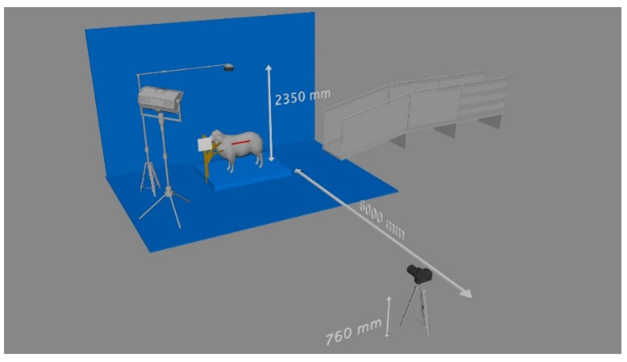
Figure 1. Experimental setup.

Figure 2. CT scan.

Figure 3. Ewe top body parameters.

Figure 4. Ewe side body parameters.

Figure 5. CT fat vs ANNs fat based on BCS.

Table 2. Descriptive statistics of training data.

Item	Minimum	Maximum	Mean	Std deviation
Fat (kg)	0.88	17.65	5.26	3.00
Lean (kg)	12.65	20.78	16.22	1.49
Bone (kg)	2.03	3.77	2.68	.32
BCS	2.0	4.5	2.72	.52
Weight (kg)	44.00	88.50	58.92	7.83
Chest width (mm)	220.3	360.2	270.2	20.8
Angle length (mm)	670.1	870.6	770.9	40.2
Body length (mm)	600.7	810.6	710.7	40.5
Side length (mm)	640.7	870.1	760.6	40.4
Front height (mm)	540.9	670.8	620.2	20.7
back height (mm)	560.1	710.6	640.0	30.0
Depth (mm)	320.6	470.0	380.2	20.6
Top length (mm)	670.5	950.7	780.6	50.4
Width (mm)	270.8	370.3	310.9	20.1
Back width (mm)	200.0	380.5	300.7	20.9
Top area (mm²)	13543	288061	197304.6	28909.4
Side area (mm²)	216830	316730	283703.6	31401.9

Table 3. Body parameters repeat test using custom-ruler (mm).

Values	Body length	Angle length	Height	Depth	Abdominal width
Max, min	+6, -15	+8, -11	+17, -12	+15, -4	+10, -13
Mean diff.	1%	1%	1%	1%	1%

Table 5. Average error % of absolute weaning and pre-mating between actual and app measurements.

Values	Angle length	Body Length	Height	Depth	Top length	Width	Side length
Weaning	5%	4%	4%	3%	5%	4%	n/a
Pre-mating	7%	3%	3%	4%	6%	5%	4%

Table 6. Rotated component matrix.

Component matrix^a
	Component
	1	2	3
BCS		.789
LW		.707
Chest width	.827
Angle length	.805
Body length	.834
Side length	.859
Height			.779
Back height			.769
Depth	.708
Top length	.736
Width	.745
Rump width	.726
Top area	.916
Side area	.935
Extraction method: Principal component analysis. Rotation method: Varimax with Kaiser normalisation.
a. 3 components extracted

Table 7. Relationships between LW and body parameters to estimate fat - MLR.

Independent Variables	R²	Equation	RMSE
LW, Chest width	0.79	-20.043 + 0.244LW + 0.401CH	1.34
LW, Angle length	0.71	-23.159 + 0.296LW + 0.141AL	1.59
LW, Body length	0.72	-21.733 + 0.301LW+ 0.129BL	1.59
LW, Side length	0.71	-21.119 + 0.293LW + 0.119SL	1.62
LW, Front height	0.68	-14.670 + 0.315LW+ 0.022FH	1.69
LW, Back height	0.68	-13.195 + 0.318LW + -0.004BH	1.69
LW, Depth	0.70	-18.764 + 0.288LW + 0.185D	1.64
LW, Top length	0.69	-17.092 + 0.310LW + 0.052TL	1.67
LW, Width	0.73	-22.113 + 0.247LW + 0.402W	1.56
LW, Rump width	0.71	-17.949 + 0.303LW + 0.175RW	1.62
LW, Top area	0.73	-16.688 + 0.291LW + 0.002TA	1.55
LW, Side area	0.72	-17.402 + 0.285LW + 0.002SA	1.58
All variables	0.80	-21.115 + 0.235LW + 0.522CH + 0.101AL + -0.042BL + 0.008SL + 0.034FH + 0.013BH + -0.067D + -0.053TL + -0.021W + -0.090RW	1.34

Table 8. Relationships between LW and body parameters to estimate fat - ANNs.

Independent variables	R²	RMSE
LW, Chest width	0.88	1.17
LW, Angle length	0.84	1.61
LW, Body length	0.83	1.36
LW, Side length	0.82	1.33
LW, Front height	0.80	1.81
LW, Back height	0.81	1.78
LW, Depth	0.85	1.47
LW, Top length	0.85	1.44
LW, Width	0.84	2.18
LW, Rump width	0.84	2.21
LW, Top area	0.84	2.21
LW, Side area	0.85	1.28
All variables	0.95	1.22

Table 9. Relationships between LW and body parameters to estimate lean - MLR.

Independent variables	R²	Equation	RMSE
LW, Chest width	0.51	10.773 + 0.156LW + -0.138CH	1.04
LW, Angle length	0.47	9.564 + 0.134LW + -0.015AL	1.09
LW, Body length	0.47	9.700 + 0.134LW + -0.019BL	1.09
LW, Side length	0.47	9.778 + 0.135LW+ -0.045SL	1.09
LW, Front height	0.47	5.919 + 0.127LW + 0.045FH	1.08
LW, Back height	0.47	7.476 + 0.129LW + 0.018BH	1.09
LW, Depth	0.47	10.112 + 0.140LW + -0.056D	1.08
LW, Top length	0.47	8.345 + 0.131LW + 0.002TL	1.09
LW, Width	0.52	12.588 + 0.164LW + -0.189W	1.03
LW, Rump width	0.48	10.146 + 0.137LW + -0.064BW	1.07
LW, Top area	0.49	9.500 + 0.139LW + -0.001TA	1.07
LW, Side area	0.47	9.303 + 0.138LW + 0.000SA	1.58
All variables	0.52	-5.109 + 0.151LW + -0.082CH + -0.004AL + 0.020BL + -0.044SL + 0.010FH + -0.004BH + -0.046D + -0.102TL + -0.004W + 0.072RW + -0.003TA + 0.001SA	1.4

Table 10. Relationships between LW and body parameters to estimate lean - ANNs.

Independent variables	R²	RMSE
LW, Chest width	0.76	1.13
LW, Angle length	0.63	1.87
LW, Body length	0.62	1.01
LW, Side length	0.73	1.11
LW, Front height	0.74	1.03
LW, Back height	0.73	1.33
LW, Depth	0.71	2.42
LW, Top length	0.63	1.09
LW, Width	0.65	1.11
LW, Rump width	0.66	1.07
LW, Top area	0.71	1.01
LW, Side area	0.72	1.09
All variables	0.79	1.20
LW, Rump width, Front height	0.77	1.26

Table 11. Relationships between LW and body parameters to estimate bone - MLR.

Independent variables	R²	Equation	RMSE
LW, Chest width	0.22	1.616 + 0.021LW + -0.006CH	0.89
LW, Angle length	0.24	0.861 + 0.018LW + 0.010AL	0.88
LW, Body length	0.24	0.952 + 0.019LW + 0.009BL	0.88
LW, Side length	0.24	0.947 + 0.018LW + 0.009SL	0.88
LW, Front height	0.23	1.133 + 0.019LW + 0.007FH	0.89
LW, Back height	0.22	1.317 + 0.019LW + 0.004BH	0.89
LW, Depth	0.25	2.152 + 0.023LW + -0.022D	0.88
LW, Top length	0.25	0.808 + 0.018LW + 0.010TL	0.88
LW, Width	0.26	2.321 + 0.026LW + -0.037W	0.87
LW, Rump width	0.22	1.553 + 0.020LW + -0.001BW	0.89
LW, Top area	0.22	1.474 + 0.019LW + -0.005TA	0.89
LW, Side area	0.22	1.458 + 0.019LW + 0.005SA	0.89
All variables	0.36	1.678 + 0.029LW + -0.035CH + -0.008AL + 0.0006BL + -0.013SL + -0.017FH + 0.019BH + -0.063D + -0.026TL + -0.067W + 0.023RW + -0.001TA + 0.000SA	0.25

Table 12. Relationships between LW and body parameters to estimate bone - ANNs.

Independent variables	R²	RMSE
LW, Chest width	0.45	2.3
LW, Angle length	0.50	2.31
LW, Body length	0.43	1.03
LW, Side length	0.41	1.05
LW, Front height	0.60	1.82
LW, Back height	0.42	1.04
LW, Depth	0.57	1.94
LW, Top length	0.65	1.15
LW, Width	0.65	1.05
LW, Rump width	0.50	1.03
LW, Top area	0.58	1.01
LW, Side area	0.56	2.22
All variables	0.75	2.40
LW, Chest width, Front height	0.59	1.2
LW, Angle length, Front height	0.46	1.12
LW, Body length, Front height	0.53	1.19
LW, Side length, Front height	0.52	2.17
LW, Depth, Front height	0.61	1.0
LW, Top length, Front height	0.53	2.36
LW, Width, Front height	0.72	1.11

Table 13. Test data prediction of 24 ewes - ANNs vs MLR vs RT.

Dependent variables	Independent variables
	MLR – R²	ANNs – R²	RT – R²
Fat	0.87 (LW, chest width)	0.90 (LW, chest width)	0.74 (LW, chest width)
Lean	0.41 (LW and width)	0.72 (LW, Rump width, Front height)	0.21 (LW, width and chest width)
Bone	0.34 (LW and width)	0.50 (LW, Width, Front height)	0.03 (LW, rump width and chest width)

* Tables may have a footer.

Table 14. Fat test data estimation in (kg) - body condition score.

CT Fat	MLR	ANNs	RT	BCS
13.867	11.240	14.062	6.92	3
12.479	9.588	10.800	6.5	2.5
7.249	7.680	7.196	5.93	3
4.390	3.631	3.639	11.51	4
6.674	6.035	6.105	8.59	3
9.066	7.157	6.372	3.5	2.5
6.209	6.974	6.125	5.53	2.5
7.919	6.230	5.608	14.12	3.5
12.329	9.850	11.521	3.98	2.5
7.242	6.364	5.874	3.83	2.5
5.117	4.656	4.324	4.05	3
5.943	6.084	5.790	8.99	3
13.034	9.876	11.809	6.1	2.5
4.451	4.185	4.036	6.63	2.5
3.742	4.141	4.007	8.27	2.5
4.513	4.518	4.379	5.16	2.5
10.940	10.129	11.774	6.62	3
7.403	6.486	5.627	6.66	2.5
6.301	7.687	6.893	5.71	2.5
5.148	5.177	5.114	10.34	3.5
5.595	5.771	5.176	8.41	3
7.114	7.567	6.620	8.12	2.5
6.616	7.314	6.411	2.67	2.5
3.525	3.653	3.666	7.687	2.5

Disclaimer/Publisher’s Note: The statements, opinions and data contained in all publications are solely those of the individual author(s) and contributor(s) and not of MDPI and/or the editor(s). MDPI and/or the editor(s) disclaim responsibility for any injury to people or property resulting from any ideas, methods, instructions or products referred to in the content.

© 2024 by the authors. Licensee MDPI, Basel, Switzerland. This article is an open access article distributed under the terms and conditions of the Creative Commons Attribution (CC BY) license (https://creativecommons.org/licenses/by/4.0/).

Copyright: This open access article is published under a Creative Commons CC BY 4.0 license, which permit the free download, distribution, and reuse, provided that the author and preprint are cited in any reuse.

MDPI Initiatives

Important Links

Choose an area of interest and we will send you notifications of new preprints at your preferred frequency.

Disclaimer