Submitted:
09 June 2023
Posted:
12 June 2023
You are already at the latest version
Abstract
Keywords:
1. Introduction
2. Materials and Methods
2.1. Sample preparation
2.2. Spectral data collection
2.3. Reference analysis
2.3.1. Higher heating value (HHV)
2.3.2. Ultimate analysis
2.4. Spectral preprocessing
2.5. Model development
3.0. Result and Discussion
3.1. Higher heating value
3.2. Ultimate analysis
3.2.1. wt.% of C
3.3.2. wt.% of H
3.3.3. wt.% of O
3.3.4. wt.% of N
3.4. Comparison with previous work
4.0. Conclusions
Author Contributions
Funding
Data Availability Statement
Acknowledgments
Conflicts of Interest
Abbreviations
| % = percentage |
| C = carbon |
| CHNS = CHNS Elemental analyzer |
| GA = genetic algorithm |
| H = hydrogen |
| HHV = higher heating value |
| LVs = latent variable number |
| Max = maximum |
| Min = minimum |
| MP = multi-preprocessing |
| MSC = multiplicative scatter correction |
| N = nitrogen |
| NT = total number of sample |
| Nc = number of sample in calibration set |
| NIRS = near infrared spectroscopy |
| Np = number of sample in validation set |
| O = oxygen |
| PLSR = partial least squares regression |
| R2 = coefficient of determination |
| R2C = coefficient of determination of calibration set |
| R2p = coefficient of determination of validation set |
| RMSEC = root mean square error of calibration set |
| RMSEP = root mean square error of prediction set |
| RPD = ratio of prediction to deviation |
| S = sulfur |
| SD = standard deviation |
| SEC = standard error of calibration set |
| SEL = standard error of laboratory |
| SEP = standard error of validation set |
| SNV = standard normal variate |
| SPA = successive projection algorithm |
| SW = selected wavenumber |
| wt.% = weight percentage |
References
- Zhang, Y.; Wang, H.; Sun, X.; Wang, Y.; Liu, Z. Separation and Characterization of Biomass Components (Cellulose, Hemicellulose, and Lignin) from Corn Stalk. BioResources 2021, 16. [Google Scholar] [CrossRef]
- Díez, D.; Urueña, A.; Piñero, R.; Barrio, A.; Tamminen, T. , Determination of hemicellulose, cellulose, and lignin content in different types of biomasses by thermogravimetric analysis and pseudocomponent kinetic model (TGA-PKM method). Processes 2020, 8, 1048. [Google Scholar] [CrossRef]
- Posom, J.; Sirisomboon, P. , Evaluation of the higher heating value, volatile matter, fixed carbon and ash content of ground bamboo using near infrared spectroscopy. Journal of Near Infrared Spectroscopy 2017, 25, 301–310. [Google Scholar] [CrossRef]
- Mierzwa-Hersztek, M.; Gondek, K.; Jewiarz, M.; Dziedzic, K. , Assessment of energy parameters of biomass and biochars, leachability of heavy metals and phytotoxicity of their ashes. Journal of Material Cycles and Waste Management 2019, 21, 786–800. [Google Scholar] [CrossRef]
- Posom, J.; Shrestha, A.; Saechua, W.; Sirisomboon, P. , Rapid non-destructive evaluation of moisture content and higher heating value of Leucaena leucocephala pellets using near infrared spectroscopy. Energy 2016, 107, 464–472. [Google Scholar] [CrossRef]
- Demirbas, A. , Hazardous Emissions from Combustion of Biomass. Energy Sources, Part A: Recovery, Utilization, and Environmental Effects 2007, 30, 170–178. [Google Scholar] [CrossRef]
- Onifade, M.; Lawal, A. I.; Aladejare, A. E.; Bada, S.; Idris, M. A. , Prediction of gross calorific value of solid fuels from their proximate analysis using soft computing and regression analysis. International Journal of Coal Preparation and Utilization 2019, 42, 1170–1184. [Google Scholar] [CrossRef]
- Sheng, C.; Azevedo, J. L. T. , Estimating the higher heating value of biomass fuels from basic analysis data. Biomass and Bioenergy 2005, 28, 499–507. [Google Scholar] [CrossRef]
- El-Sayed, S. A.; Mostafa, M. , Pyrolysis characteristics and kinetic parameters determination of biomass fuel powders by differential thermal gravimetric analysis (TGA/DTG). Energy conversion and management 2014, 85, 165–172. [Google Scholar] [CrossRef]
- Huang, C.; Han, L.; Yang, Z.; Liu, X. , Ultimate analysis and heating value prediction of straw by near infrared spectroscopy. Waste Manag 2009, 29, 1793–1797. [Google Scholar] [CrossRef]
- Adnan, A.; Horsten, D. V.; Pawelzik, E.; Morlein, A. D. , Rapid Prediction of Moisture Content in Intact Green Coffee Beans Using Near Infrared Spectroscopy. Foods 2017, 6. [Google Scholar] [CrossRef]
- Roger, J.-M.; Mallet, A.; Marini, F. , Preprocessing NIR Spectra for Aquaphotomics. Molecules 2022, 27, 6795. [Google Scholar] [CrossRef]
- Maraphum, K.; Saengprachatanarug, K.; Wongpichet, S.; Phuphuphud, A.; Posom, J. , Achieving robustness across different ages and cultivars for an NIRS-PLSR model of fresh cassava root starch and dry matter content. Computers and Electronics in Agriculture 2022, 196. [Google Scholar] [CrossRef]
- Posom, J.; Phuphaphud, A.; Saengprachatanarug, K.; Maraphum, K.; Saijan, S.; Pongkan, K.; Srimai, K. Real-time measuring energy characteristics of cane bagasse using NIR spectroscopy. Sensing and Bio-Sensing Research 2022, 38. [Google Scholar] [CrossRef]
- Phuphaphud, A.; Saengprachatanarug, K.; Posom, J.; Taira, E.; Panduangnate, L. , Prediction and Classification of Energy Content in Growing Cane Stalks for Breeding Programmes Using Visible and Shortwave Near Infrared. Sugar Tech 2022, 24, 1497–1509. [Google Scholar] [CrossRef]
- Posom, J.; Sirisomboon, P. , Evaluation of the higher heating value, volatile matter, fixed carbon and ash content of ground bamboo using near infrared spectroscopy. Journal of Near Infrared Spectroscopy 2017, 25, 301–310. [Google Scholar] [CrossRef]
- Posom, J.; Saechua, W. In Prediction of elemental components of ground bamboo using micro-NIR spectrometer, IOP Conference Series: Earth and Environmental Science, 2019; IOP Publishing: 2019; p 012063.
- Skvaril, J.; Kyprianidis, K. G.; Dahlquist, E. , Applications of near-infrared spectroscopy (NIRS) in biomass energy conversion processes: A review. Applied Spectroscopy Reviews 2017, 52, 675–728. [Google Scholar] [CrossRef]
- Zhang, K.; Zhou, L.; Brady, M.; Xu, F., Yu; Wang, D. , Fast analysis of high heating value and elemental compositions of sorghum biomass using near-infrared spectroscopy. Energy 2017, 118, 1353–1360. [Google Scholar] [CrossRef]
- Xue, J.; Yang, Z.; Han, L.; Chen, L. , Study of the influence of NIRS acquisition parameters on the spectral repeatability for on-line measurement of crop straw fuel properties. Fuel 2014, 117, 1027–1033. [Google Scholar] [CrossRef]
- Jiao, Y.; Li, Z.; Chen, X.; Fei, S. Preprocessing methods for near-infrared spectrum calibration. Journal of Chemometrics 2020, 34. [Google Scholar] [CrossRef]
- Posom, J.; Maraphum, K.; Phuphaphud, A. , Rapid Evaluation of Biomass Properties Used for Energy Purposes Using Near-Infrared Spectroscopy. In Renewable Energy-Technologies and Applications, IntechOpen: 2020.
- Yun, Y.-H.; Li, H.-D.; Deng, B.-C.; Cao, D.-S. , An overview of variable selection methods in multivariate analysis of near-infrared spectra. TrAC Trends in Analytical Chemistry 2019, 113, 102–115. [Google Scholar] [CrossRef]
- Broad, N.; Graham, P.; Hailey, P.; Hardy, A.; Holland, S.; Hughes, S.; Lee, D.; Prebble, K.; Salton, N.; Warren, P. , Guidelines for the development and validation of near-infrared spectroscopic methods in the pharmaceutical industry. Handbook of vibrational spectroscopy 2002, 5, 3590–3610. [Google Scholar]
- Nakawajana, N.; Posom, J.; Paeoui, J. , The prediction of higher heating value, lower heating value and ash content of rice husk using FT-NIR spectroscopy. Engineering Journal 2018, 22, 45–56. [Google Scholar] [CrossRef]
- Assis, C.; Ramos, R. S.; Silva, L. A.; Kist, V.; Barbosa, M. H. P.; Teofilo, R. F. , Prediction of Lignin Content in Different Parts of Sugarcane Using Near-Infrared Spectroscopy (NIR), Ordered Predictors Selection (OPS), and Partial Least Squares (PLS). Appl Spectrosc 2017, 71, 2001–2012. [Google Scholar] [CrossRef]
- Li, Z.; Song, J.; Ma, Y.; Yu, Y.; He, X.; Guo, Y.; Dou, J.; Dong, H. , Identification of aged-rice adulteration based on near-infrared spectroscopy combined with partial least squares regression and characteristic wavelength variables. Food Chemistry: X 2023, 17, 100539. [Google Scholar] [CrossRef] [PubMed]
- Shetty, N.; Gislum, R. , Quantification of fructan concentration in grasses using NIR spectroscopy and PLSR. Field Crops Research 2011, 120, 31–37. [Google Scholar] [CrossRef]
- Conzen, J. Multivariate Calibration: A practical guide for developing methods in the quantitative analytical chemistry. Ettlingen, Germany: BrukerOptik GmbH, 2006. [Google Scholar]
- Pitak, L.; Sirisomboon, P.; Saengprachatanarug, K.; Wongpichet, S.; Posom, J. , Rapid elemental composition measurement of commercial pellets using line-scan hyperspectral imaging analysis. Energy 2021, 220. [Google Scholar] [CrossRef]
- Xia, Z.; Zhang, C.; Weng, H.; Nie, P.; He, Y. , Sensitive wavelengths selection in identification of Ophiopogon japonicus based on near-infrared hyperspectral imaging technology. International journal of analytical chemistry 2017, 2017. [Google Scholar] [CrossRef] [PubMed]
- Zhang, C.; Liu, F.; Kong, W.; Zhang, H.; He, Y. , Fast identification of watermelon seed variety using near infrared hyperspectral imaging technology. Transactions of the Chinese Society of Agricultural Engineering 2013, 29, 270–277. [Google Scholar]
- Liu, D.; Sun, D.-W.; Zeng, X.-A. , Recent advances in wavelength selection techniques for hyperspectral image processing in the food industry. Food and Bioprocess Technology 2014, 7, 307–323. [Google Scholar] [CrossRef]
- Santos-Rufo, A.; Mesas-Carrascosa, F.-J.; García-Ferrer, A.; Meroño-Larriva, J. E. , Wavelength selection method based on partial least square from hyperspectral unmanned aerial vehicle orthomosaic of irrigated olive orchards. Remote Sensing 2020, 12, 3426. [Google Scholar] [CrossRef]
- Maraphum, K.; Ounkaew, A.; Kasemsiri, P.; Hiziroglu, S.; Posom, J. , Wavelengths selection based on genetic algorithm (GA) and successive projections algorithms (SPA) combine with PLS regression for determination the soluble solids content in Nam-DokMai mangoes based on near infrared spectroscopy. Engineering and Applied Science Research 2022, 49, 119–126. [Google Scholar]
- Jiang, Q.; Chen, Y.; Guo, L.; Fei, T.; Qi, K. , Estimating soil organic carbon of cropland soil at different levels of soil moisture using VIS-NIR spectroscopy. Remote Sensing 2016, 8, 755. [Google Scholar] [CrossRef]
- Williams, P.; Manley, M.; Antoniszyn, J. , Near infrared technology: Getting the best out of light. African Sun Media: 2019.
- Zornoza, R.; Guerrero, C.; Mataix-Solera, J.; Scow, K. M.; Arcenegui, V.; Mataix-Beneyto, J. , Near infrared spectroscopy for determination of various physical, chemical and biochemical properties in Mediterranean soils. Soil Biology and Biochemistry 2008, 40, 1923–1930. [Google Scholar] [CrossRef] [PubMed]
- Alzagameem, A.; Bergs, M.; Do, X. T.; Klein, S. E.; Rumpf, J.; Larkins, M.; Monakhova, Y.; Pude, R.; Schulze, M. , Low-input crops as lignocellulosic feedstock for second-generation biorefineries and the potential of chemometrics in biomass quality control. Applied Sciences 2019, 9, 2252. [Google Scholar] [CrossRef]
- Den, W.; Sharma, V. K.; Lee, M.; Nadadur, G.; Varma, R. S. , Lignocellulosic biomass transformations via greener oxidative pretreatment processes: Access to energy and value-added chemicals. Frontiers in chemistry 2018, 6, 141. [Google Scholar] [CrossRef] [PubMed]
- Weyer, L. , Practical guide to interpretive near-infrared spectroscopy. CRC press: 2007.
- Hasan, M.; Haseli, Y.; Karadogan, E. , Correlations to predict elemental compositions and heating value of torrefied biomass. Energies 2018, 11, 2443. [Google Scholar] [CrossRef]
- Zoghlami, A.; Paës, G. , Lignocellulosic biomass: Understanding recalcitrance and predicting hydrolysis. Frontiers in chemistry 2019, 7, 874. [Google Scholar] [CrossRef] [PubMed]
- Ge, X.; Chang, C.; Zhang, L.; Cui, S.; Luo, X.; Hu, S.; Qin, Y.; Li, Y. , Conversion of lignocellulosic biomass into platform chemicals for biobased polyurethane application. In Advances in bioenergy, Elsevier: 2018; Vol. 3, pp 161-213.
- Sirisomboon, P.; Funke, A.; Posom, J. , Improvement of proximate data and calorific value assessment of bamboo through near infrared wood chips acquisition. Renewable Energy 2020, 147, 1921–1931. [Google Scholar] [CrossRef]
- Lestander, T. A.; Rhén, C. , Multivariate NIR spectroscopy models for moisture, ash and calorific content in biofuels using bi-orthogonal partial least squares regression. Analyst 2005, 130, 1182–1189. [Google Scholar] [CrossRef]
- Han, K.; Gao, J.; Qi, J. , The study of sulphur retention characteristics of biomass briquettes during combustion. Energy 2019, 186, 115788. [Google Scholar] [CrossRef]
- Cagnon, B.; Py, X.; Guillot, A.; Stoeckli, F.; Chambat, G. , Contributions of hemicellulose, cellulose and lignin to the mass and the porous properties of chars and steam activated carbons from various lignocellulosic precursors. Bioresource Technology 2009, 100, 292–298. [Google Scholar] [CrossRef] [PubMed]
- Posom, J.; Sirisomboon, P. , Evaluation of lower heating value and elemental composition of bamboo using near infrared spectroscopy. Energy 2017, 121, 147–158. [Google Scholar] [CrossRef]
- Nakawajana, N.; Posom, J. In Comparison of analytical ability of pls and svm algorithm in estimation of moisture content, higher heating value, and lower heating value of cassava rhizome ground using FT-NIR spectroscopy, IOP Conference Series: Earth and Environmental Science, 2019; IOP Publishing: 2019; p 012032.
- Zhang, K.; Zhou, L.; Brady, M.; Xu, F.; Yu, J.; Wang, D. , Fast analysis of high heating value and elemental compositions of sorghum biomass using near-infrared spectroscopy. Energy 2017, 118, 1353–1360. [Google Scholar] [CrossRef]
- Nhuchhen, D. R. , Prediction of carbon, hydrogen, and oxygen compositions of raw and torrefied biomass using proximate analysis. Fuel 2016, 180, 348–356. [Google Scholar] [CrossRef]

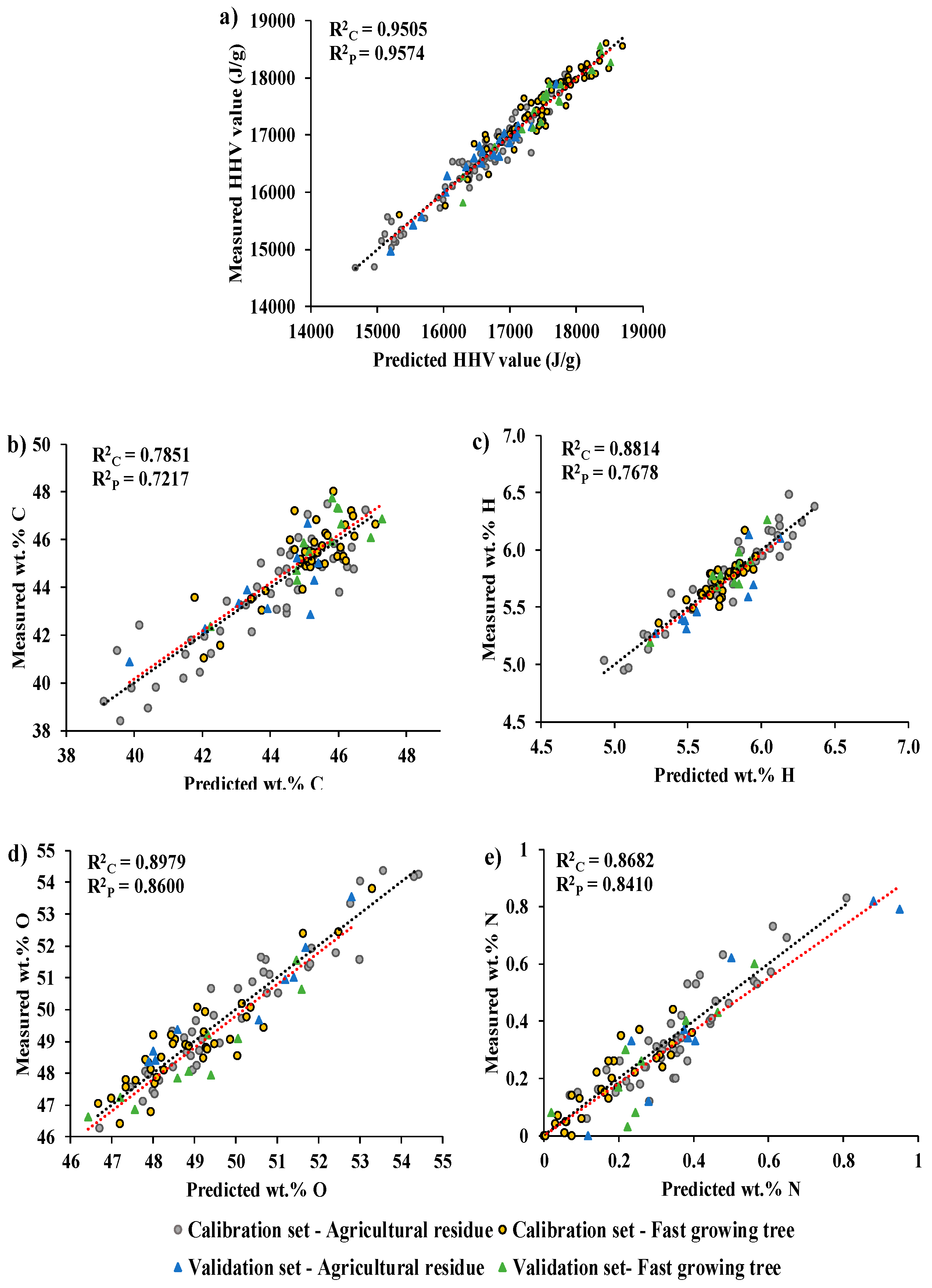
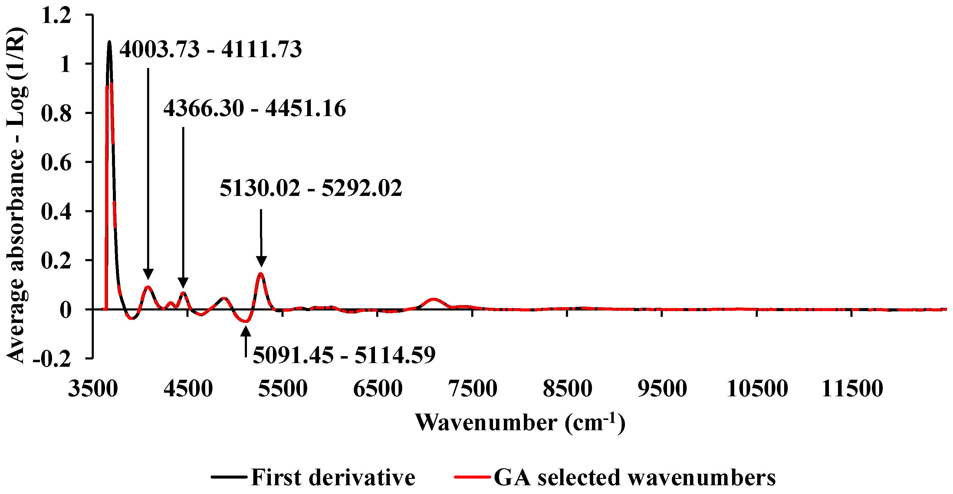
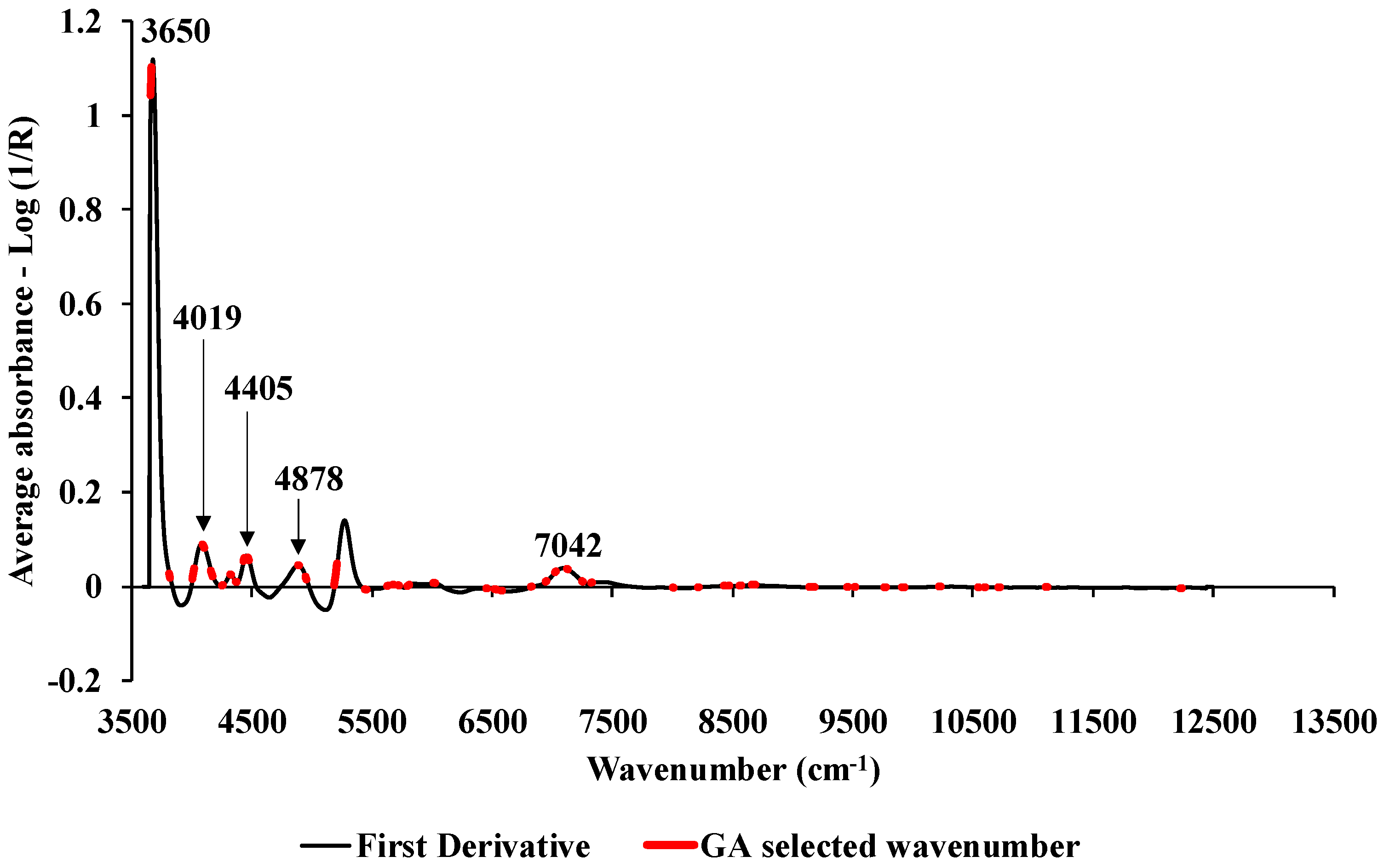
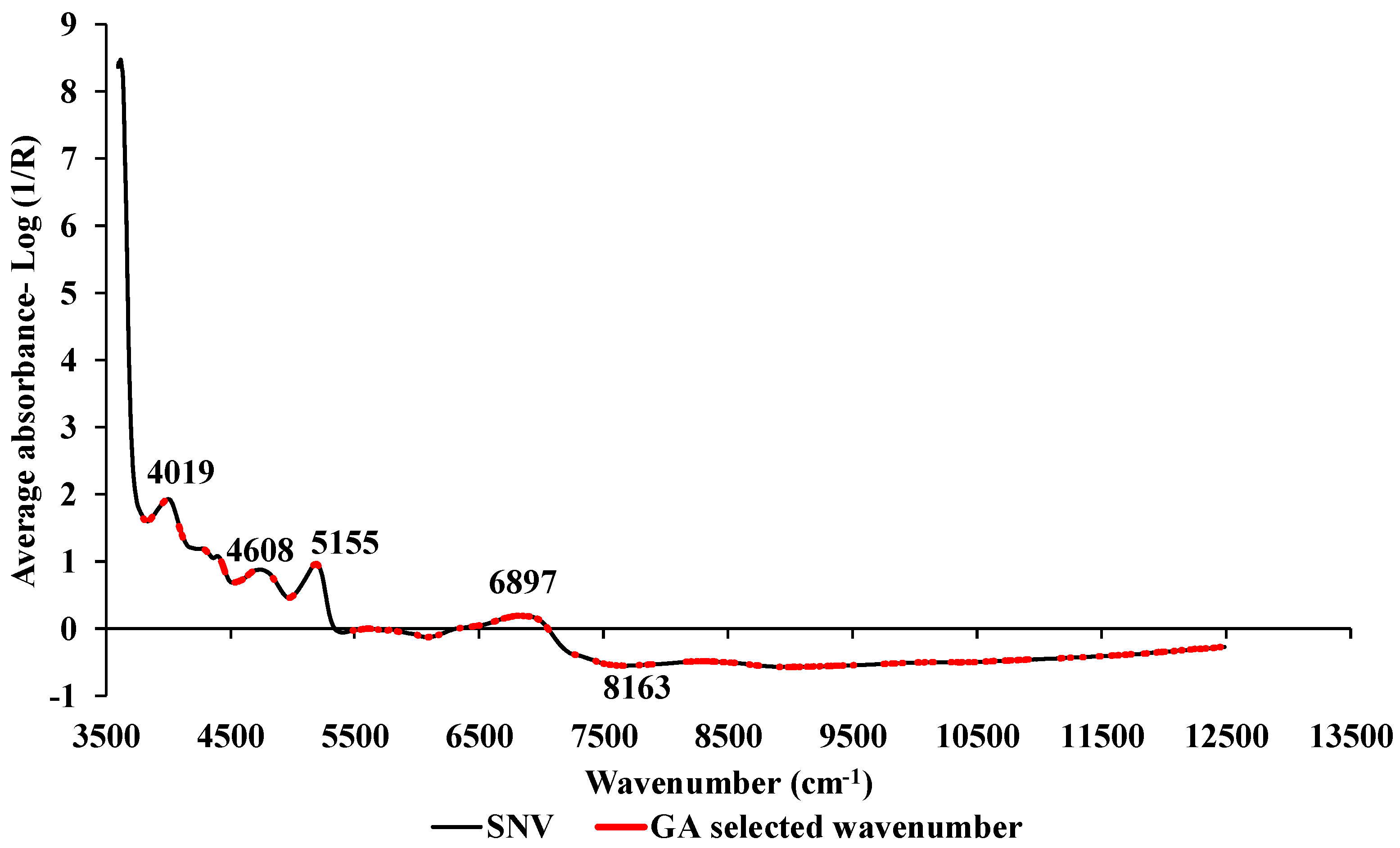
| Category | Particular | HHV (J/g) | C (wt.%) | N (wt.%) | H (wt.%) | O (wt.%) |
|---|---|---|---|---|---|---|
| Fast growing tree | Alnus nepalensis | 17932 | 45.9115 | 0.3115 | 5.7255 | 48.0515 |
| Pinus roxiburghii | 18349 | 46.8367 | 0.0606 | 5.8283 | 47.2744 | |
| Bombusa vulagris | 17310 | 45.6132 | 0.2327 | 5.7536 | 48.4005 | |
| Eucalyptus camaldulensis | 17105 | 44.5536 | 0.0896 | 5.6164 | 49.7404 | |
| Bombax ceiba | 17077 | 44.8557 | 0.3162 | 5.8179 | 49.0102 | |
| Agricultural residue | Zea mays (cob) | 17297 | 44.7794 | 0.2488 | 5.7619 | 49.2100 |
| Zea mays (shell) | 16409 | 45.6518 | 0.4318 | 6.2113 | 47.7050 | |
| Zea mays (stover) | 16753 | 44.3988 | 0.7069 | 5.6697 | 49.2245 | |
| Oryza sativa | 15417 | 40.4261 | 0.4996 | 5.3042 | 53.7701 | |
| Saccharum officinarum | 17029 | 43.6413 | 0.1047 | 5.7047 | 50.6827 |

Disclaimer/Publisher’s Note: The statements, opinions and data contained in all publications are solely those of the individual author(s) and contributor(s) and not of MDPI and/or the editor(s). MDPI and/or the editor(s) disclaim responsibility for any injury to people or property resulting from any ideas, methods, instructions or products referred to in the content. |
© 2024 by the authors. Licensee MDPI, Basel, Switzerland. This article is an open access article distributed under the terms and conditions of the Creative Commons Attribution (CC BY) license (https://creativecommons.org/licenses/by/4.0/).


