Preprint
Article

Software Product Lines Maintenance using Many Objectives Optimization Techniques

Altmetrics

Downloads

163

Views

88

Comments

0

A peer-reviewed article of this preprint also exists.

Submitted:

12 June 2023

Posted:

12 June 2023

You are already at the latest version

Alerts
Abstract
Currently, software development is more associated with families of configurable software rather than the single implementation of a product. Due to the numerous possible combinations in a software product line, testing these families of software product lines (SPLs) is a difficult undertaking (SPL). Moreover, the presence of optional features makes the testing of SPLs impractical. Several features are presented in SPLs, but due to the environment's time and financial constraints, these features are rendered unfeasible. Testing subsets of configured products is thus one approach to solving this issue. In order to reduce testing effort and get better results, alternative methods of testing SPLs are required, such as the combinatorial interaction testing (CIT) technique. Unfortunately CIT method produces unscalable solutions for large size SPLs with excessive constraints. The CIT method costs more because of feature combinations. The optimization of the various conflicting testing objectives, such as reducing the cost and configuration number, have also been considered. In this article, we have proposed a search-based software engineering solution using multi-objective optimization algorithms (MOEAs). In particular, the research is applied to different types of MOEA methods; Indicator-Based Evolutionary Algorithm (IBEA), Multi-objective Evolutionary Algorithm based on Decomposition (MOEA/D), Non-Dominated Sorting Genetic Algorithm II (NSGAII), NSGAIII, and Strength Pareto Evolutionary Algorithm 2 (SPEA2). The results of the algorithms are examined in the context of distinct objectives and two quality indicators. The results revealed how feature model attributes, implementation context and the number of objectives affect the performance of the algorithms.
Keywords: 
Subject: Computer Science and Mathematics  -   Software

1. Introduction

Software companies have used effective testing techniques like automated testing to improve the quality of their software products. However, derived products are selected from a broad product platform, the testing procedure for a software product line (SPL) could be complicated and expensive. Moreover, the testing process for SPL is challenging due to the large number of product variants which is needed to be tested. By producing test cases automatically, the testing procedure can be made more effective and scalable. Software engineering problems can be solved computationally using a metaheuristic strategy, and this is what search-based software engineering (SBSE) represents [1]. The search-based software testing (SBST) assist in generating the optimal test cases in term of time and cost using metaheuristics techniques [2,3]. Due to the redundancy of test cases, the testing process becomes time-consuming. The various testing optimization methodologies help to identify the issues related to resource utilization and component coordination. Due to the exponentially growing features in the product line, a classification for product sampling approaches have been proposed which are based on algorithm type and coverage criteria [4].
The process of developing a product line is difficult now because there are thousands of variation points. [6,7]. Using interactive tools and procedures that are appropriate for huge data sets and interrelationships, the intriguing efforts can be resolved [8]. The testing of the software product line is a challenging activity, but it will be optimal if all products in a product line are configured properly [9]. However, it is complex to generate configurations. SPL testing is a hard process because of the complex composition and design of the product [10]. In reality, certain features enable millions of variation configurations. For instance, a video player product line’s feature model (FM) with 71 features enables it to configure more than 1.65x10¹³ different products. In order to reduce a product line’s test suites, it will be unable to test every product in an SPL at a reasonable cost. The focus of this article is to optimize a large number of test cases in software product lines. For this, five different multi-objective evolutionary algorithms have been selected to optimize the SPL test suite. In this context, we addressed the following research questions in this article.
RQ 1: How the proposed method, which uses multi-objective optimization (in the case of four objectives optimization), will provide the solutions?
RQ 2: Which algorithm, employing the four objectives optimization, is the best fit to produce the optimized results?
The rest of the article is organized as follows: section 2 provides related work on software product lines testing and multi-objective algorithms, section 3 describes how multi-objective help to optimize SPL testing. Section 4 presents the method description and testing objectives and section 5 describes the experimental setup and results. Lastly, sections 6 and 7 present the conclusion and future directions of our work.

2. Software product Line Engineering

Software product lines engineering technique utilize to make it possible to develop a variety of products quickly, affordably, and with excellent quality [11]. This methodology uses a number of features to produce particular systems or products [12]. Throughout the SPL process, the reusable components are combined to generate the desired product.
The product line technique has improved the quality of the software [13]. The development life cycle objects, such as requirement specification documents, conceptual diagrams, architectures, reusable components, testing and maintenance techniques, are merged to meet the process’ goals [13]. The reusability of components is essential to the product line’s methodology. The methodology is divided into two main phases, the first phase is “Domain Engineering”, wherein the analysis, design, and implementation of that domain are used to generate core assets. The second phase is the “Application Engineering”, where the customers’ unique specifications are used to develop final products [13]. The workflow for software product line engineering has been shown in Figure 1. The development of core assets occurs during the domain engineering phase of SPL engineering, whereas their setup takes place during the application engineering phase. Variation points exist that aid in product configuration [6]. When compared to conventional development methods, domain and application engineering efforts are more successful. To ensure the productivity efficiently, the application engineering procedures must operate well [6].

3. Related Work

The use of search-based approaches in SPL engineering is not common [1]. SPL testing is improved by using the delta modeling approach where the deltas calculate the product similarity. Using this technique, the dissimilar product would be tested next. This approach has been evaluated in the automotive domain regarding SPL testing [14]. The similarity-based prioritization has been introduced with the aim to choose diverse products concerning features which are needed to be tested with the coverage of features during SPL testing [15]. A genetic algorithm-based framework using fault technique of test specifications reuse. The proposed technique was applied to four different SPL models to evaluate the capability of the framework [16]. Krüger et al. [17] discussed mutation operators which are appropriate to find variability faults and enhance the competence of the existing or conventional operators. For the regression testing of SPL, a retest selection technique was proposed. This approach relies on delta modeling which calculates the commonality and variability of product line variants and different versions of variants. A solution is proposed by using change impact analysis to distinguish between variants and versions of variants where there is a need to retest the changed dependencies in the selection of test cases for re-execution [18].
A hybrid multi-objective optimization algorithm called SMTIBEA was proposed. This technique merges the indicator-based evolutionary algorithm (IBEA) with the satisfiability modulo theories (SMT) solving methodology. The approach was applied to large SPLs to compare the state of the artwork. The proposed approach obtained better results in terms of the expressiveness of constraints [19]. The SPL test list generation scheme which relies on Harmony Search (HS) algorithm called SPL-HS was recommended. The approach originates the minimum number of test cases for all features that depend on the required interaction degree. The obtained results show that the SPL-HS technique has the capability to contest with existing SPL testing approaches to generate optimal results [20]. The validation partial configurations approach has been proposed to deliberate different cases like selection, attributes and constraints of features and this technique were applied with the industry variant tool known as pure::variants. This approach helps to validate the partial configurations for different real-world software product lines [21]. Wang et al. presented his work with a focus on test cases minimization [22]. They took advantage of a genetic algorithm with accumulated function with these determinants 1) test cases numbers, 2) coverage in terms of pairs and 3) find faults. Another approach was also introduced by [23], where they discussed the test cases prioritization. In addition to their work, they prescribed a cost function. They worked on a random search technique in contrast to a genetic algorithm using (1+1) Evolutionary Algorithm. Their evaluation process focused on different genetic algorithm configurations assigned with different weights. In another research work, they mentioned considerations like resources and execution cost [23]. Ensan et al. recommended an approach using genetic algorithm inclusion with composed function to calculate the cost and number of errors [24]. Henard et al. worked on the same approach using a genetic algorithm with a function to deal with contrary objectives [25]. The configuration of features and selection approaches has also been described [26]. The selection techniques were prescribed by them to work on various objectives. For instance, similar techniques like evolution and user preferences were recommended by [27,28,29].
Authors have mentioned [30,31] their work on SPLs evolution run time and execution. While the issue of SPLs configuration was discussed formally by other researchers who mainly focus on cost, user preferences, and feature model violations rules [32,33,34,35,36]. Sayyed [37,38] recommended an approach for product lines configuration evaluating distinct multi-objective evolutionary algorithms in terms of different aspects like product selection, the breached rules in feature models, the utilized features and the exposed faults during the testing process. The use of multi-objective algorithms generated testing results based on different defined criteria. For example, Lopez [39] suggested Pareto solutions describe the pairwise coverage. Regardless of this, other researchers presented the genetic algorithm using some aggregated functions. In addition to other factors, the pairwise coverage criteria have basic importance in testing. Henard [40] advocated test data generation for mutation testing. In our work, the same operators have been used to originate products in terms of test cases for the testing process.
As a result of the aforementioned assessment of gaps or weaknesses in the literature 1) the amount of test cases and test suites for the SPL testing procedure has to be decreased, 2) It can be difficult to optimize multiple objectives simultaneously when dealing with a multi-objective optimization problem. The size of the test cases is one of the key issues with product line testing. So, in order to do product line testing completely, all generic components and even all potential product versions must be tested. In fact complete testing become challenging as the number of product variants increases [3,44]. As a result, the system undergoes more testing as more products are generated. At this stage, the main focus is on minimizing redundant tests in order to reduce testing effort. The relationship between produced and derived goods from the same requirements should be taken into account when minimizing test redundancy [3,44].
In SPL, the generation of configurations is a multi-objective issue. As a result, the activity of SPL testing can be viewed as the development of configurations, which is a multi-objective problem. As a result, it is possible to view the testing of the product line as a multi-objective problem. Although SPL testing using the CIT approach can be a single-objective problem, but there is also a need to optimize other objectives, such as minimizing the number of configurations, maximizing the number of features, and minimizing the cost of testing these products [27]. As optimization of many objectives environments can be difficult, though, as achieving one objective may prevent the optimization of other objectives. The results of the implementation of multi-objective evolutionary algorithms (MOEAs) in SPL testing will be used to obtain any interventions made by software testers.
This study establishes the rationale for employing MOEA algorithms in SPL testing. The proposed algorithm will help to find more accurate and beneficial results in terms of performance, accuracy, and cost, the suggested work will measure MOEA. This research will assist the SPL testing industry to utilize the MOEAs to aid the SPL testing process. In addition, the adopted MOEAs will be competent in setting the precedence of future generation and selection of test cases with an aim to reduce test cases numbers to cope with the time limit environment. Hence, the ultimate goal of this research is to maximize the coverage of valid features in a product line that needs to be tested. In this work, the SPL testing technique comprises the optimization of multiple objectives, therefore there may need to compromise some objectives to optimize one objective. Hence, the optimization of conflicting objectives is also considered as a limitation. The evaluation of configurations can take time in hours or days hence it is computationally expensive. Therefore, it is required to discover other approaches besides the configuration evaluation technique in order to find faults and robust results rather than the CIT approach.

4. Optimization for SPL Testing using Multiobjective Evolutionary Algorithms

Hence, the optimization of conflicting objectives is also considered as a limitation. The evaluation of configurations can take time in hours or days hence it is computationally expensive. Therefore, it is required to discover other approaches besides the configuration evaluation technique in order to find faults and robust results rather than the CIT approach.

4.1. Method Description

The different definitions concerning the research problem have been outlined as required.

4.1.1. Definition 1 (Feature Model)

A Feature Model is a set of m Boolean features with certain constraints, where a feature model (FM) expressed as F = { f 1 ,   f 2 ,   . ,   f m } while set L = { c 1 ,   ... ,   c n } represents the constraints for the features. A constraint C can be fulfilled by seeing whether the imperatives or constraints are satisfied. Mendonca [41] mentioned that a feature model can be expressed into a Boolean representation using constraints solvers to analyze a feature model. Such Boolean expressions are defined as the combination of logical clauses. Therefore, a clause is set forth for a feature model and it literally specifies either a feature is true ( f j -selected) or false ( f j -not selected). Hence to describe a FM, the following Boolean expression can be used.
F M = Λ k i = 1 ( j [ 1 ; n ] l j ) , w h e r e   l j = f j   o r   f ¯ j
The use of search-based approaches in SPL engineering is not common [1]. SPL testing is improved by using the delta modeling approach where the deltas calculate the product similarity.

4.1.2. Definition 2 (Configuration)

The features recommended by a product of a SPL are configurations. Therefore, in a configuration, either there will be a selection of particular features or maybe not while satisfying the rules of defined constraints. For a product of SPL, a configuration is considered as a set C = { ± f 1 ,   ... ,   ± f n } , where + f i feature shows the presence in FM for the respective product, while f i   represents the absence of that feature. However, here it is important that a configuration will be valid if the constraints of FM are satisfied.

4.1.3. Definition 3 (Configuration Suite)

Configuration suite consists set of valid configurations and is represented as C S = { C 1 , ..   . , C m } , where each object C i   presents a valid configuration.

4.1.4. Definition 3 (Coverage Criteria)

Coverage Criteria is defined as a set of t-sets covered by the configuration, where the t-set can be defined as a configuration with a certain number of valid and invalid features as defined in the last sections. The given below ratio is to describe the pair-wise coverage of a configuration suite C S = { C 1 , ..   . , C m }.
# i = 1 m T t , C i # T t , F M
where T t , C i   is the set of t-sets encompassed by the configuration C i (i.e., t-sets entailed within the configuration ( C i ), where T t , F M , is indicative of the set of all the possible t-sets of the FM and where the cardinality of the set A is depicted by # A . For t-wise testing, the above coverage ratio is considered as 1 using classical approaches because these approaches cover all t-tests of a feature model [42-44].
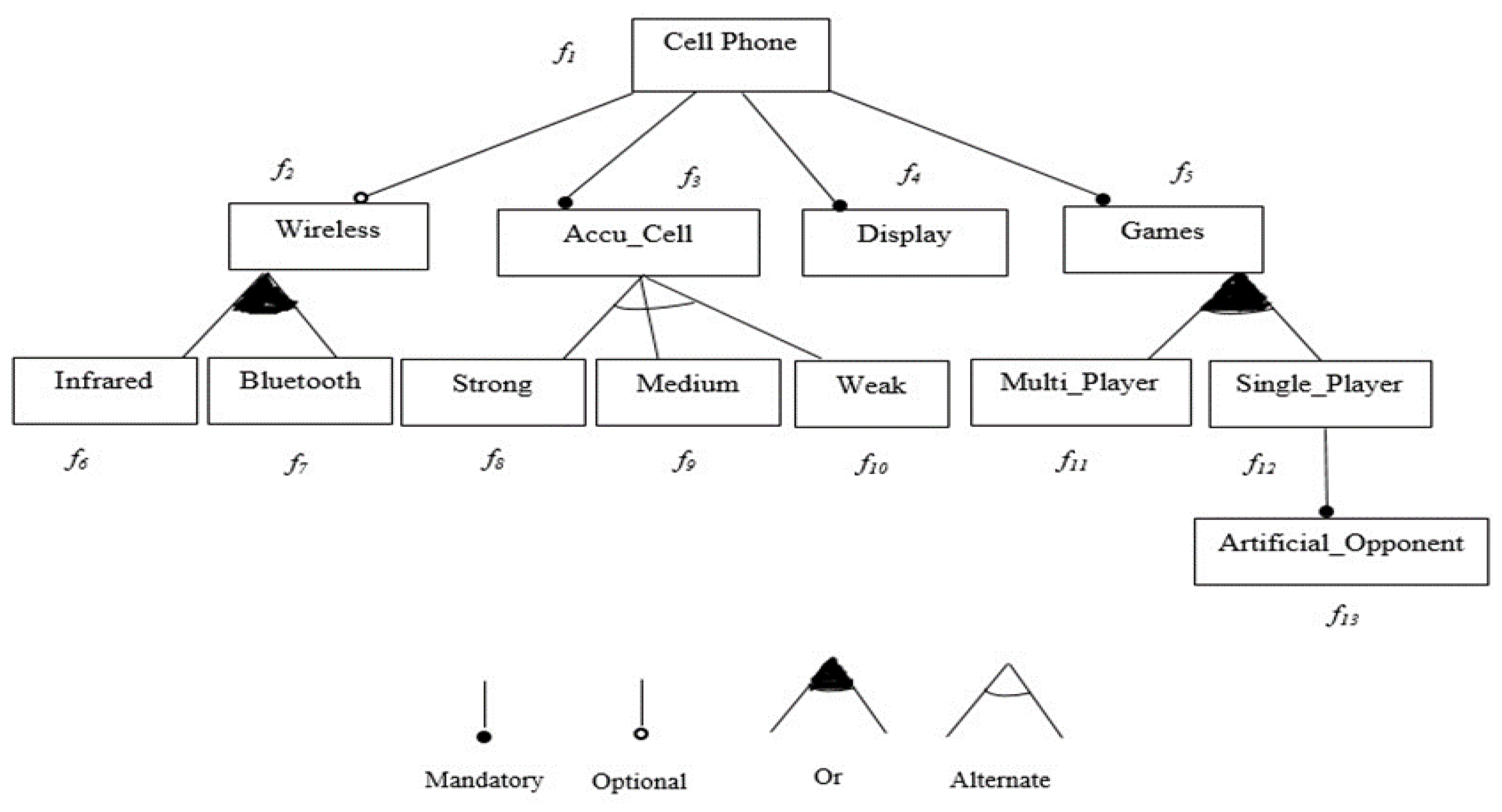
For example, the feature model depicted in Fig 2, can have the following different number of configurations.
C 1 = { + f 1 , + f 2 , + f 3 , + f 4 , + f 5 , + f 6 , f 7 , + f 8 , f 9 , f 10 , + f 11 , f 12 , f 13 }
C 2 = { + f 1 , + f 2 , + f 3 , + f 4 , + f 5 , f 6 , + f 7 , f 8 , + f 9 , f 10 , + f 11 , f 12 , f 13 }
C 3 = { + f 1 , f 2 , + f 3 , + f 4 , + f 5 , f 6 , f 7 , f 8 , f 9 , + f 10 , + f 11 , f 12 , f 13 }
C 4 = { + f 1 , + f 2 , + f 3 , + f 4 , f 5 , + f 6 , f 7 , f 8 , + f 9 , f 10 , f 11 , f 12 , f 13 } .

4.1.5. Definition 5 (Individual)

An individual is expressed by a set of configuration suite i.e., I = { C 1 , ,   C n } as I generate solutions for the problem, while a gene produced by a valid configuration and MOEA, the Genetic Algorithm (GA) basically manages the set of individuals. Hence, the search space of all possible sets of configurations that are capable of holding configurations in a SPL has been acquired.

4.1.6. Definition 5 (Population)

A Population is a set of individuals, where a gene is shown by a valid configuration. The genetic algorithm (GA) deals with a set of individuals considered as population. Hence, a large search space of sets of valid configurations that exist in a SPL is obtained.
The Materials and Methods should be described with sufficient details to allow others to replicate and build on the published results. An example of the Cell-Phone feature model has been described in Figure 2 which shows a total of 13 numbers of features represented by f 1 ,   f 2 ,   . ,   f 13 . The above Figure 2 shows Cell Phone as a root feature of the feature model and this root feature will be included in every product configuration. In this FM, Accu_Cell, Display and Games features are considered mandatory features. These three features would be present in each configuration. There exists an exclusive-or relation between Accu_Cell with its child features. It means that there would be an inclusion of explicitly on one out of three features i.e., Strong, Medium or Weak.
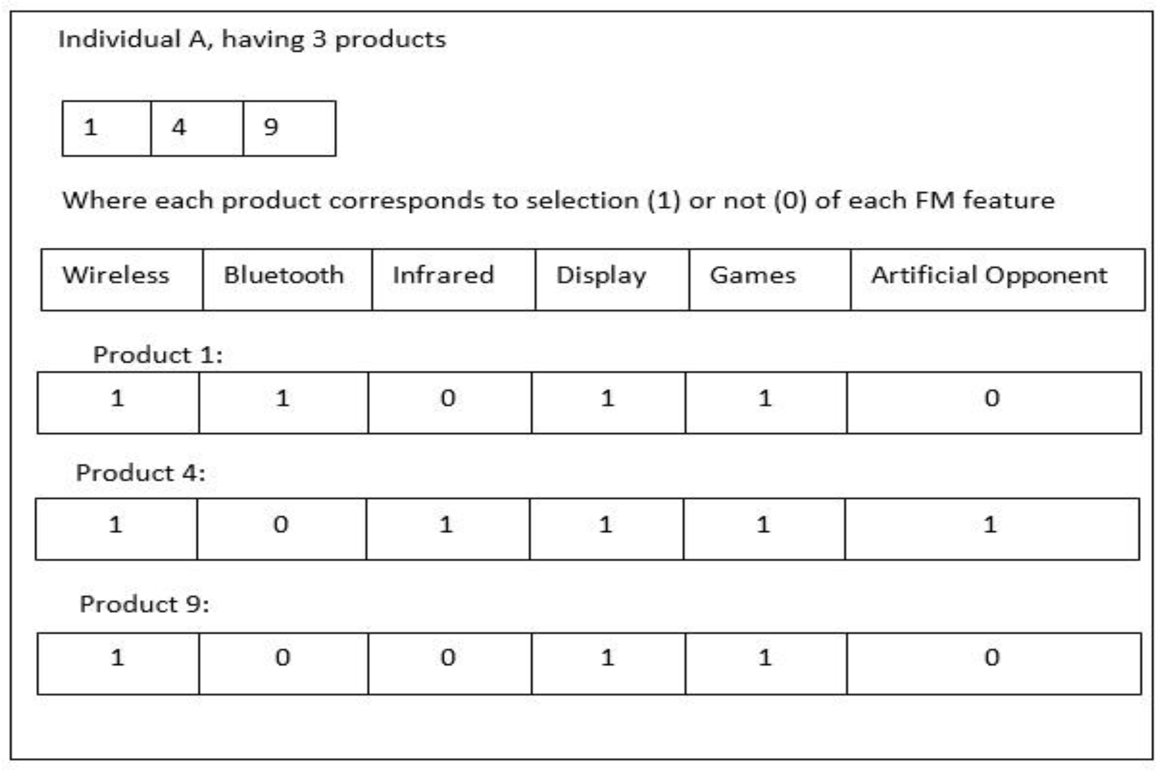
However, in the case of Multi-Player and Single Player features form an inclusive-or relation, which means for a valid configuration, there is a selection of at least one feature among two features. Artificial Opponent is considered as a mandatory child feature for the Single Player. For the main Cell Phone parent, the Wireless feature is taken as an optional child feature, therefore, its selection may be optional. The Wireless feature has Infrared and Bluetooth child features and making an inclusive-or association. This means if any configuration contains a Wireless feature, then it must have at least one child feature to be included or selected. There persist three crosstree constraints in the Cell Phone product line. As long as there is an important selection for a Multi_Player feature that cannot be considered with the Weak feature, hence for this Wireless feature, the selection is mandatory. At the end, for the Bluetooth feature, the Strong feature selection is also compulsory. The set of n products represents the individual population as exemplified in Figure 3. In that example, every single X contains 3 products, based on the integer numbers: (1, 4, and 9). A binary vector represents each product and its every element represents a feature of a feature model. The value (0) represents a feature which is not selected and (1) represents the corresponding feature. In the example, the product 1 does not contain the features of Infrared and Artificial Opponent
For the achievement of optimization criteria, it is difficult to identify a SPL configuration fulfilling a number of potentially conflicting objectives. The issue becomes intensified when a configuration suite fulfilling testing goals comprising of a set of configurations need to be generated, which is assumed to be the actual issue needed to be handled. The constraint solving techniques and multi-objective evolutionary algorithms are part of our approach and to produce configuration suites, these approaches need to be applied in a balancing way so that fulfilling of four testing objectives could be analyzed at the same time. For SPLs, the configuration generation problem is modeled as a search problem. In the proposed approach, sets of configurations are modeled as individuals and configurations as genes. It is also indicative of likely operations on the individuals and on the objective function. Hence, search-based approaches are enabled to fix the configuration generation problem. To eliminate the invalid configurations from the search space, the constraint solving technique is used.
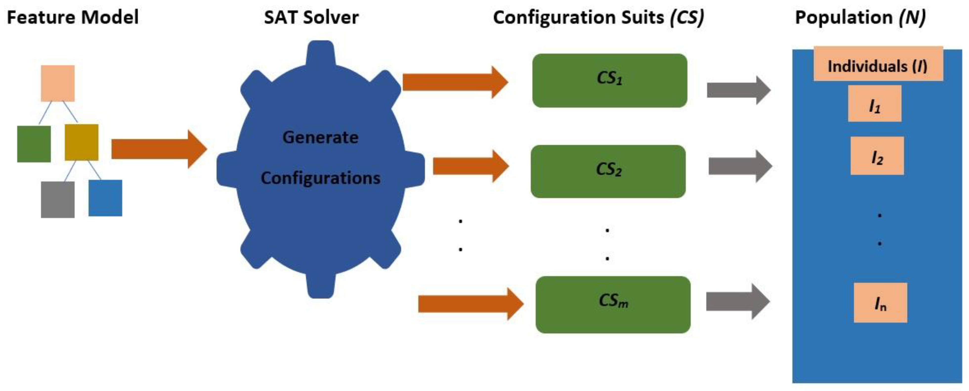
To provide the maximum size of an individual, there is a need to specify the size of the population. A set of 1, ..., m configurations randomly selected from all the valid configurations towards the feature model (FM) is represented by each individual. The evolution of the population into a new one is considered as the second step of the approach. The crossover and mutation are the next steps. The individuals are created using mutation and crossover operators to complete the new population till the time it attains its size n. The aim of crossover is to create two offspring from their selected parents. The user initially specifies a certain probability, where mutation takes place on the offspring. Afterward, the fitness of these two offspring is analyzed and the new population is integrated with these two new individuals. Finally, the new population replaces the existing population and it continues to the next generation. Upon termination of the algorithm, the best fitness value of the individual is obtained. The proposed approach has been shown in Figure 4.

4.2. Objectives Definition

For the achievement of optimization criteria, different objectives are defined, which might create a conflict with each other during the optimization process. In the proposed research, the following objectives are considered.

4.2.1. Maximize the Pairwise Coverage

This objective ensures the maximum level of pairwise coverage from the selected products, where Coverage Criteria is defined as a set of t-sets covered by the configuration, where the t-set can be defined as a configuration with a certain number of valid and invalid features as defined in the last sections. It is represented as
O 1 ( a ) = coverage ( a )
where the coverage function is used to calculate the number of pair of features covered by set a = { P 1 , ,   P n } .

4.2.2. Minimize the Number of Products

Each product represents a test case. Therefore, the number of products should be minimized. The goal of this objective is to minimize the number of products:
O 2 ( a ) = cardinality ( a )
where, cardinality function determines in returning the number of products n of a = { P 1 , ,   P n }   and it is assumed that a feature exists implicitly at most once in each product. The cardinality of a feature also demonstrates that how many times a feature is included in a configuration.

4.2.3. Testing Cost

The testing cost of products has been minimized using the following objective function.
O 3 ( a ) = cost ( a )
This function makes sure that the testing cost will be minimized with the help of the above defined objective. The different resources and costs are required by each feature to be tested. In this regard, each feature is allocated a value indicative of an estimate of its testing cost. Therefore, the sum of the cost of its features is presumably equivalent to the cost of testing for one configuration. In other words, if the cost of the feature f i is symbolized by cost ( f i ) , then a configuration C = { ± f 1 ,   ... ,   ± f n }   possesses a cost equal to:
cos t ( C ) = i = 1 n p ( i ) cos t ( i ) ,   where   p ( i ) = { 1           i f + f i 0           i f f i
The cost of the m configurations is composed by summing up the cost of a test configuration suite. Hence, the given below equation gives the cost of C S = { C 1 , ..   . , C m } :
cos t ( C S ) = i = 1 m cos t ( C i )

4.2.4. Maximizing Number of Features

The population is Configuration Suite { C 1 , C 1 ..   . , C k } use to count the number of positive features in a vector of Configuration C i = { + f 1 ,   . , f n , f 1   , f n } . The goal of this function is to count features. This objective can be defined as
C S k = i n j m λ ( P F ( i , j )
where λ ( P F ( i , j ) = 1 , if i n ( P F ( i , j ) > 1 , else=0
The CS represents the configuration suite and PF shows the product features.

5. Experiments

In this section, we discussed the framework adopted, data collection procedure and parameter settings.

5.1. Framework Adopted

This section describes how the experiments were designed and conducted: SPL feature models, algorithms implementation and quality indicators for the comparison of the algorithms. The approach employed is like as adopted in our recent research work [46]. For evaluation and implementation, five multi-objective algorithms have been selected: IBEA [47], MOEA/D [48], NSGAII [49], NSGAIII [50], SPEA2 [51]. There exists a free and open-source Java library framework called “The MOEA Framework”. It is used for both single and multi-objective optimization algorithms. The MOEA Framework endures aiding genetic algorithms, grammatical evolution, particle swarm optimization, genetic programming, and differential evolution [52]. This framework consists of operators and solutions for optimization problems and it also implements quality indicators like hypervolume.
The selected algorithms are being configured and re-executed to generated and report the results. As mentioned above in equation 1, the Boolean formula of a feature model is encoded into a SAT solver to resolve a configuration whether a configuration is valid or invalid for a feature model. The formula is applied as a conjunction form for all constraints and evaluated to true (valid) values for the satisfied constraints by the solver.

5.2. Data Collection

The six feature models are selected with dissimilar sizes and obtained from Software Product Line Tools (SPLOT) [10]. Table 1 displays the various attributes of these selected feature models. The six feature models have been considered for four objectives optimization, having smaller, medium and larger size features to analyze the results. The feature models characteristics are mentioned in Table 1. The first column shows different feature models, the second represents the number of features, third and fourth column shows the number of configurations, number of valid pairs respectively.

5.3. Parameters Selection

The parameters settings are adopted before initiating the experiments. The fixed parameters have been finalized in the beginning to have the constant result and may have the possibility of comparing the efficiency of the algorithms involved in experiments. The opted parameters are the size of the population, the maximum number of evaluations, and the size of FM, crossover and mutation rates as shown in Table 2.

6. Results and Discussion

We performed experiments that relied on the experimental methodology discussed in previous sections. First, the results of Pareto fronts are presented with tuned parameters on selected SPLOT feature models configurations.

6.1. Pareto Front Solutions

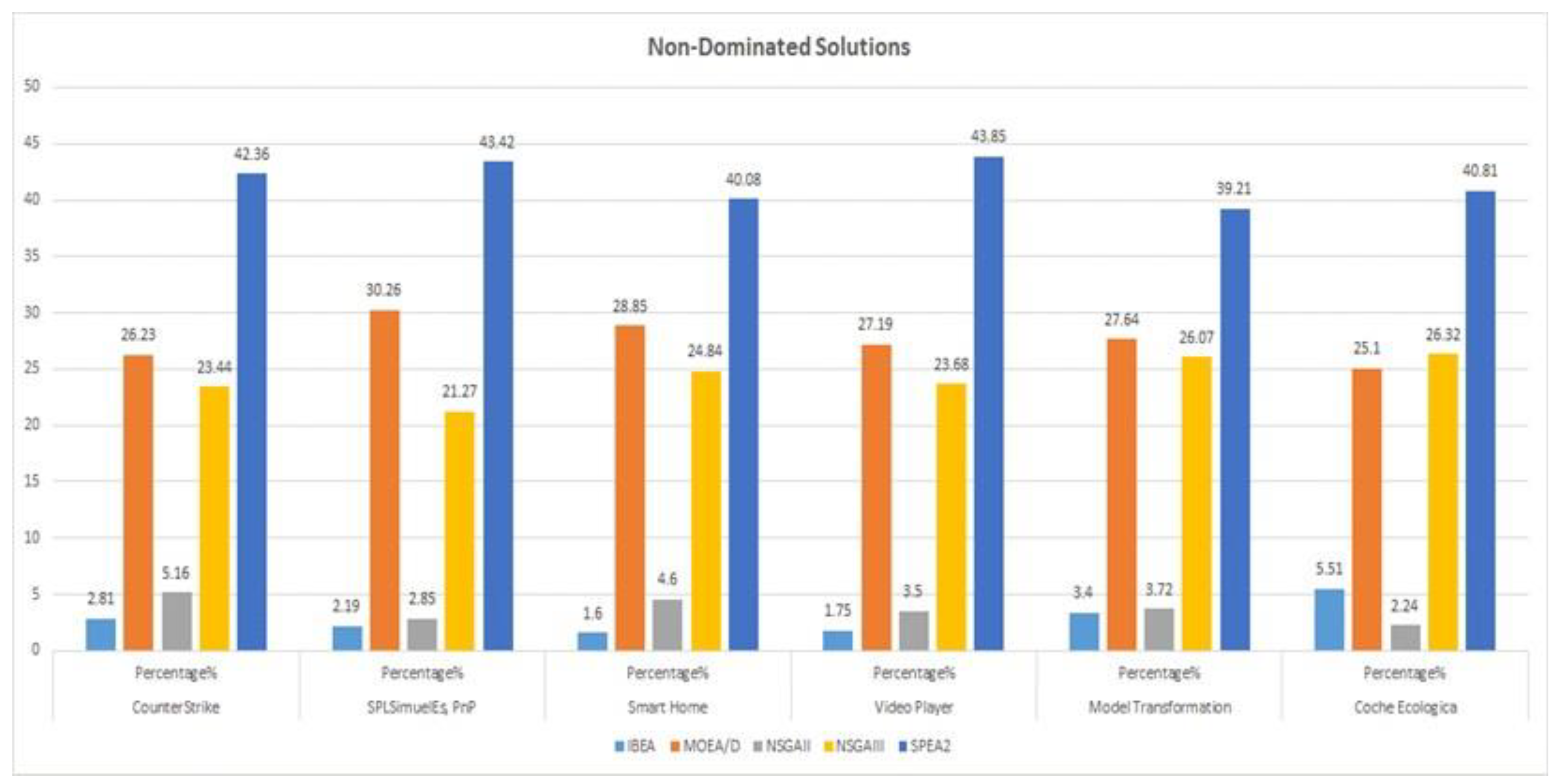
The results of the proposed research are shown and analyzed in this section. The non-dominated solutions are presented in Table 3 based on the Pareto dominance concepts [53]. Table 3 presents the main results generated by each algorithm and feature model for many objectives optimization. The column 2 shows the total number of solutions in global pareto front PFtrue, formed by the non-dominated solutions generated by executions of all five algorithms. However, other columns present the number of non-dominated solutions generated by individual algorithm known as PFcontribution which are present in PFtrue and values in parenthesis show the percentage of non-dominated solutions by each algorithm as compare to global solutions PFtrue.
The preliminary analysis of Table 3 shows that IBEA and NSGAII algorithms generate the certain number of solutions in PFtrue in consideration of the used objectives. All the algorithms used in this research find these solutions for all feature models in all runs. The IBEA algorithm generates minimum number of solutions for SmartHome v2.2 and Video Player feature models. However, in the case of other feature models that are more solutions are originated by IBEA and for the larger size feature model Coche Ecologico, it generates a greater number of non-dominated solutions resulting in 27 solutions as compared to other feature models. In case of NSGAII, diversity of solutions has been observed like for small size feature model Counter Strike, it originates from 24 solutions while in the case of larger size feature model Coche Eoclogico, it generates the minimum number of solutions i.e., 11. Similarly, to observe the results of NSGAIII, MOEA/D and SPEA2, these three algorithms generate the good number of non-dominated solutions for all feature models. From the Table 3, it simply analyzes that all the algorithms work effectively to optimize the four objectives problem.
Figure 5 shows the distinct percentage values for non-dominated solutions generated by five different MOEAs. It is obvious from Figure 4 that the SPEA2 algorithm generates maximum percentages of solutions in all selected six feature models. However, MOEA/D is also able to generate a good amount of percentage solutions for the mentioned FMs in Table 3. For MOEA/D, the solutions percentages originated for Counter Strike, SPL SimulES PnP, Smart Homev2.2, Video Player, Model Transformation and Coche Ecologico are 26.23, 30.26, 28.85, 27.19, 27.64 and 25.10 respectively. Figure 5 also describes that NSGAIII contributed well in producing the good percentage values of non-dominated solutions, while IBEA and NSGAII percentage solutions are not satisfiable as compared to the results of other MOEAs in percentage.

6.2. Results Generated By Quality Indicators

The evaluation process for the results of MOEAs is carried by using quality multi-objective indicators and statistical analysis as discussed by [54,55]. In this research work, two quality indicators have been selected to evaluate the results: Hypervolume [56], Spacing [57]. There is possibility that the efficiency of MOEAs may have an effect with four objectives, therefore, to measure better performance of MOEAs these two quality indicators have been utilized to determine the spread, convergence and smaller space for non-dominated solutions generated by the algorithms regarding to Pareto front [55,58].
Table 4 represents the hypervolume and spacing indicators with their average and standard deviation values respectively for 30 PFcontribution sets generated by each algorithm. To establish the quantitative analysis of the results values, the above-mentioned quality indicators have been utilized. These quality metrics help to originate good quality values [56]. The first column of Table 4 represents the hypervolume and spacing indicators, while other columns represent the feature models and different algorithms to calculate the average and standard deviation values using the mentioned indicators. The best values are represented in bold in Table 4.
For hypervolume, the higher values are considered as the best while minimum values take into account as the best for spacing. To analyze the hypervolume values for Counter Strike FM, it is discovered from Table 4 that MOEA/D and SPEA2 algorithms originate the best average and standard deviation values (0.7094, 0.0129) and (0.7022, 0.0165) respectively for the Counter Strike FM. Comparatively, NSGAIII results are also considered better (0.6498, 0.0113). However, in the case of IBEA (0.2826, 0.1162) and NSGAII (0. 0.6029, 0.0234), the generated hypervolume and spacing values are considered as less number of solutions.
For SPL SimulES, PnP FM, it can be deduced from Table 4 that NSGAIII values are not desirable in terms of average and standard deviation (0.5413, 0.0176) and the same behavior is displayed by IBEA and NSGAII showing values (0.2698, 0.0954) and (0.4659, 0.0314) respectively. MOEAD generates best values (0.6524, 0.0150) in contrast to other MOEAs. The values of SPEA2 are considerable to create the optimal values of average and standard deviation (0.6390, 0.0155).
In the case of Smart Homev2.2 FM, nearly the same average values with a minor difference of standard deviation (0.6885, 0.0160) and (0.6843, 0.0198) can be generated by both the MOEA/D and SPEA2. NSGAIII remained deliberate in terms of producing good result values (0.6052, 0.0300) for Smart Homev2.2 FM. Nonetheless, the performance of IBEA and NSGAII is observed as not satisfactory as they generated (0.3460, 0.1105) and (0.5742, 0.0353) values.
While considering the results of Video Player FM, the SPEA2 and MOEA/D both can produce almost the same average values with the insignificant difference of standard deviation (0.6961, 0.0155) and (0.6864, 0.0193). NSGAIII stays deliberate with respect to producing desirable result values (0.6085, 0.0262) for Smart Homev2.2 FM. On the other hand, the IBEA and NSGAII delivered unsatisfactory performance and generate (0.3659, 0.0969) and (0.5795, 0.0108) values of average and standard deviation.
After analyzing the results of Model Transformation FM, the MOEA/D and SPEA2 both can generate approximately the same average values but the minor difference of standard deviation values (0.6009, 0.0146) and (0.6136, 0.021). NSGAIII is found better to originate good result values (0.5276, 0.021) for Smart Homev2.2 FM. On the contrary, unacceptable performance is demonstrated by IBEA and NSGAII and generated values are (0.36, 0.0771) and (0.4677, 0.0256) respectively.
When the results of Coche Ecologico results are being investigated, it is found that approximately the same average values were generated by both the MOEA/D and SPEA2 with a slight change in standard deviation (0.4868, 0.0048) and (0.5025, 0.0013). Moreover, NSGAIII yields good result values (0.4541, 0.0329) for Smart Homev2.2 FM. Though the IBEA and NSGAII illustrate the poor performance generates (0.3257, 0.0802) and (0.3227, 0.0107) values respectively.
To discuss the results of spacing values, from Table 4 it is examined that for all feature models SPEA2 algorithm originates the best average and standard deviation values using the spacing metric. However, the MOEA/D and NSGAIII algorithms also generate good values of average and standard deviation.
To conclude Table 4, it is determined that the SPEA2 and MOEA/D can produce better values. It is worth mentioning that NSGAIII is also found good in producing a desirable result for most of the feature models. Nevertheless, unsatisfactory performance is revealed by IBEA and NSGAII as compared to other three algorithms.

6.3. Fitness Values for Four Objectives Optimization

Table 5 presents the fitness values of solutions for the four objectives mentioned in the above section. These fitness values of four objectives are selected from the results of the experiments. The first column of Table 5 shows the feature models and other columns represent the MOEA algorithms with their four objectives values.
The five algorithms IBEA, MOEA/D, NSGAII, NSGAIII, and SPEA2 generate fitness values for each objective. The objective one is represented by O1 which aims to maximize the pairwise coverage. The second objective i.e., minimization of product number is shown by O2. The O3 describes objective three, which is utilized to reduce the testing cost. The fourth objective is to maximize the richness of features is represented by the O4. The bold values represent the best-optimized values in comparison to other objectives values. To accomplish the maximum fitness values of O1 objective (pairwise coverage), the other three objectives O2 (minimize the number of products), O3 objective (testing cost) and O4 (richness of features) values have to compromise as shown in Table 5. To follow the same approach in order to have the best minimum fitness values for objective O2, the other three objectives like O1, O3 and O4 need to be settled. The relevant method would be adopted to have the best fitness values for objectives O3 and O4. The best fitness values for the three objectives are shown as bold in Table 5. Besides, the evolution of the objectives, the normalized objectives values over the generations of the algorithm are presented. Since all the four objectives are transformed into the optimization of the problems. It is noted that our approach is not limited to this balance. Thus, the tester or user may set a different balance according to his needs to optimize the testing process of the software product line.
Table 6 provides the analysis through the MOEAs with the optimal results using both indicators against each feature model. Table 6 inferences are determined from the results of Table 4. For Counter Strike feature model, it is explored that MOEA/D, SPEA2, and NSGAIII algorithms originate the best values using hypervolume and spacing indicators. But in the case of SPL SimulES, PnP, it is observed that MOEA/D and SPEA2 are the best algorithms to generate the optimal results using the hypervolume.
But using the spacing indicator for SPL SimulES, PnP FM, the MOEA/D, SPEA2 and NSGAIII algorithms are capable of producing better values. Similarly, the case of Smart Homev2.2 FM can be observed, where three MOEAs like MOEA/D, SPEA2 and NSGAIII are the best algorithms to generate the optimized results employing the hypervolume and spacing. For the Video Player FM, the better values using hypervolume are originated by the MOEA/D, SPEA2, and NSGAIII. However, for the Video Player feature model, these better results are obtained only by MOEA/D and SPEA2 using spacing. While, in the case of Model Transformation FM, the same results as those of Smart Homev2.2, MOEA/D, SPEA2 and NSGAIII algorithms are the best values generators using the hypervolume and spacing.
To analyze Table 6, it is examined that for Coche Ecologico FM, the MOEA/D, SPEA2, and NSGAIII have the best values using hypervolume but after utilizing the spacing, only the MOEA/D and SPEA2 algorithms produced good results. To conclude Table 6, the best optimal results are generated by the MOEA/D, SPEA2 and NSGAIII in most of the feature models.

6.4. Discussion of Results and Answers to Research Questions

It is considered that the solutions generated by every algorithm relied on the related fitness values. The solutions associated with the best results are analyzed to complete the SPL testing assessment, as it is also the overall objective of the research. The ability to generate optimal values for four objectives are clearly depicted by the findings revealed in the previous tables. The outcomes of experiments have the potential to identify better solutions for all the objectives under consideration. Although some disparities may not be statistically meaningful, it can be seen that the approach is a settlement among the conflicting objectives. Hence, due to certain parameters, it is likely to compromise the four objectives. It is worth indicating that the aforementioned results are accomplished by the proposed approach through a reasonable number of generations (500 generations).
Different parameters can have an effect to minimize the number of products, which can be the answer to the first question. To find optimal solutions, the quality testers can gain insight through this direction as to why the testing optimization techniques were adopted. But, there are some considerable cases, where systems reliability is higher than the justification for test cases. This is the benefit of our proposed methodology, which has the capacity to produce various solutions in terms of coverage as well. The choice would be in the hand of the tester in terms of adopting the better MOEA for good performance. The single objective algorithms produce one solution, which may not be an ideal selection in our case where multi objectives need to be optimized. The testers can define the priorities to select the values of different operators like the crossover rate and mutation rate to affect the experiment results of different product lines.
The best solutions are identified to assess each feature model. The quality indicators like hypervolume and spacing from the optimization field are also utilized.
In consideration of Research Question 2, the results have a clear impact regarding the performance of the algorithms with four objectives optimization as discuss in detail in different Tables. Here in this part of the Chapter with four objectives, the versatility in the generated results are obtained. However, it is determined that for all SPL feature models, the IBEA generated the worst results in terms of optimization. The MOEAD, SPEA and NSGAIII performed well in all cases of feature models with the small, medium and larger size.
Table 4 presents the analyses about the percentage of non-dominated solutions generated by the different MOEAs. Again, the SPEA2 surpasses and originates the maximum percentage of non-dominated solutions for all FMs. Similarly, MOEA/D and NSGAIII also produce a better percentage of solutions. However, the numbers of solutions percentages in the case of IBEA and NSGAII are not comparatively found to be good and generate less percentage of non-dominated solutions.
Table 5 reasoning with the average and standard deviation results of hypervolume and spacing quality indicators obliged in the proposed approach, SPEA2 also achieved the best results using hypervolume and spacing quality indicators. This means the SPEA2 algorithm provides more optimal solutions to the tester with various and ultimate values of fitness using statistical methods like average and standard deviation. It represents that MOEA/D and SPEA2 values are more optimal.
Table 6 represents the best fitness values regarding the different MOEAs, it can be observed to have the best value for a particular objective, there may need to compromise the other objectives values. So, the proposed approach has the capacity to generate the optimal fitness values in order to optimize the four objectives like to maximize the pairwise coverage, reduce the number of products, minimize the testing cost and maximize the feature richness.
It is analyzed from the results mentioned in different tables that three algorithms (SPEA2, MOEA/D, and NSGAIII) have accomplished better results. Nevertheless, the IBEA and NSGAII performance with respect to originating the optimal values is not satisfactory. All algorithms except IBEA and NSGAII tried to achieve maximum coverage besides minimizing the numbers of test cases. For future work, IBEA and NSGAII would be investigated more as tweaking the parameter values may help to generate good results.
To sum it up, the three MOEAs algorithms (MOEA/D, SPEA2, and NSGAIII) have the capacity to generate optimal solutions for the four objectives optimization approach when compared with single objective approaches.
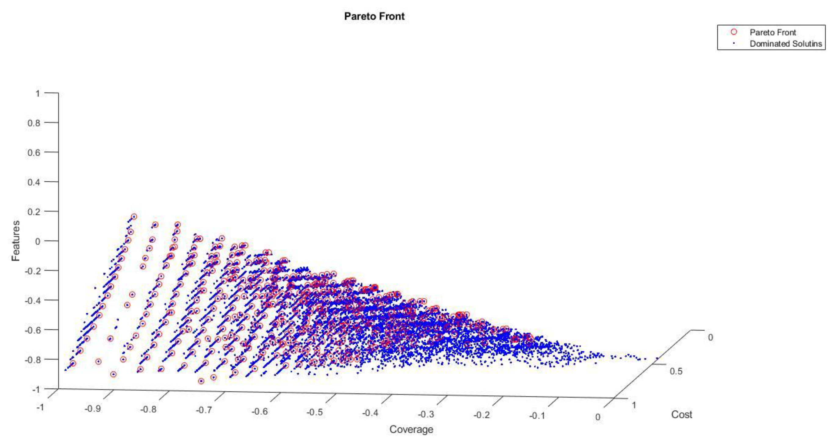
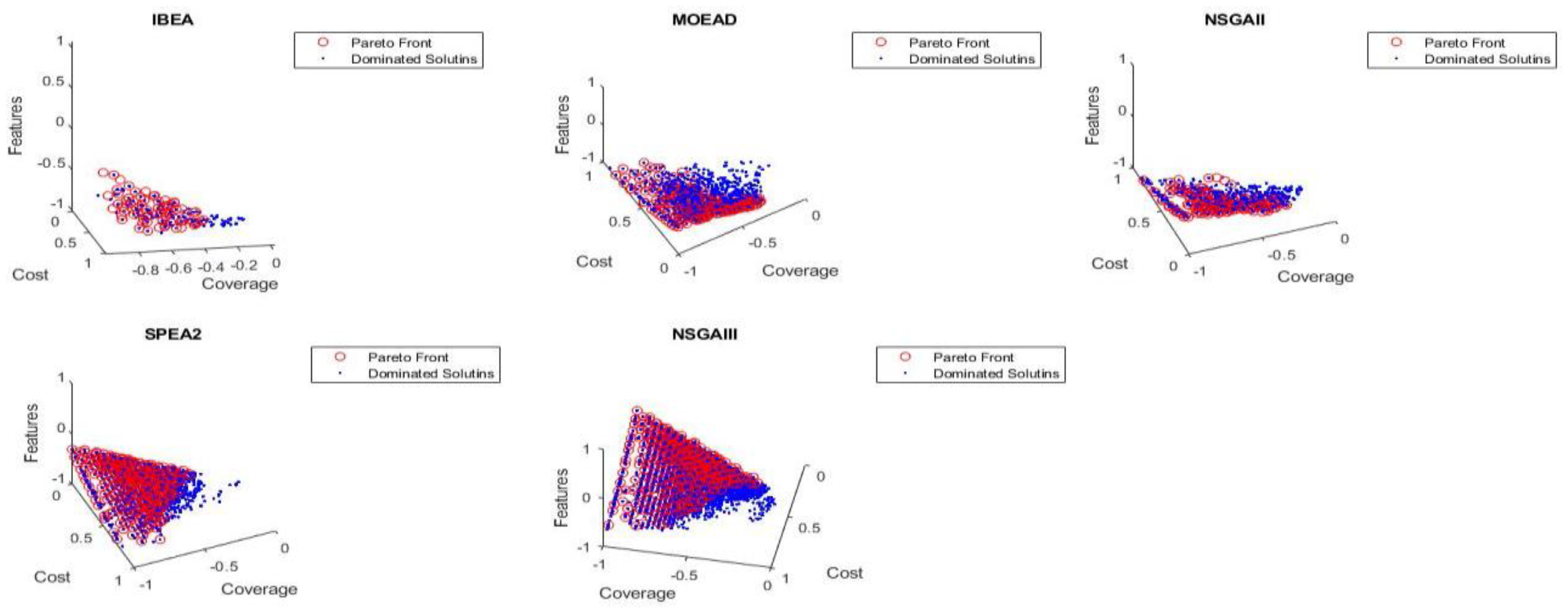
Figure 6 and Figure 7 represent the global and local Pareto fronts of Counter Strike feature model only using five multi-objectives evolutionary algorithms (IBEA, MOEA/D, NSGAII, NSGAIII and SPEA2) in case of four objectives optimization approach. Here only three objectives points are represented due to unavailability of four axis representation. The Figures shows the non-dominated Pareto fronts obtained after experiments.

7. Results

This section will be discussing the findings of the experiments and evaluations, which were performed. Moreover, the results of four objectives experiments lead to the answering of the questions of the proposed research. The advantage over the single objective approach is one achievement that is observed in the researcher’s work during evaluation [24]. The results generated are varied whereby containing good solutions using multi-objective algorithms. As per testing goals, there is a possibility that the tester may prioritize a single objective at the end because he needs to choose the extreme points or solutions.
In the case of four objectives, the comparison of the experiment shows that it does not change the cost in the required number of the product. Although, there were constraints on testing activities, for example, problems related to contractual and development, MOEA/D and SPEA2 have the ability to perform better in contrast to other MOEAs. In this manner, a diversity of solutions will be obtained, where the tester will be able to choose the best one based on the performance and requirements. In a condition, where fast execution is required, SPEA2 is the relatively right choice as FMs have a maximum number of products. The SPEA2 should be used in the interest of the tester as the tester is more inclined towards the best tradeoffs of the solution, as it has a higher number of non-dominated solutions.

7.1. Practical Implications

The different multi-objective algorithms have been utilized for the implementation of this approach. The algorithms used within the framework are IBEA, MOEA/D, NSGA-II, NSGAIII, and SPEA2. The presented approach is equally compatible with other testing approaches and with other evolutionary algorithms. T-wise testing and other operators like mutation and crossover could be used, which is also possible in future work. The four objectives are proposed to test the approach by conducting experiments. As an outcome, it is figured out that the best tradeoff between the evaluated objectives is represented by the good solutions produced.

7.2. Threats to Validity

It is believed that the sizes of the software product lines are the main challenge to our research. Yet, the software product lines, which are utilized to express the proposed approach has the ability to generate productive solutions with the capability to win over the testing optimization of the feature model. The approach has been assessed to concede scalability; the purpose is to supply with a large number of products that will be tactically handled by MOEA algorithms. The concept should be examined in the future through different experiments with a considerably even larger size of feature models to compare those used in our proposed work.
There exists a limitation that can possibly be adopted in the experiments conducted in the future to get results using different parameter settings like population size, crossover and mutation rate. It is always considered a difficult task to choose parameters for the algorithm. In order to minimize the associated threats, the recommendation offered by [59] would be considered. The iteration of the experiment was 30 as there are fixed variations which existed in the search algorithm. The iterations are performed with the intention to minimize the possibility that these results are not achieved accidentally. The evolution procedure of fitness affected the time of execution of algorithms, where machine hardware and running environment would be helpful in reducing the time while scaling the implementation to a larger feature model. The implementation of the SAT solver helps to generate the configurations from an FM and confirm their validity with respect to coverage.
To conclude, it is worth indicating that the aforementioned results are accomplished by the proposed approach through a reasonable number of generations (500 generations). Since thousands of executions can be adopted by the search-based approaches to be effective and successful, this can be hence considered as an achievement of the approach [44]. For future work authors want to extend their research using the optimization techniques mentioned in the research work of different researchers [60,61,62,63,64,65,66].

Author Contributions

All authors have read and agreed to the published version of the manuscript.

Funding

The author has received funding for this research work through the project number: IFP22UQU4320619DSR113

Data Availability Statement

Data will be available upon reasonable request.

Acknowledgments

The authors extend their appreciation to the Deputyship for Research & Innovation, Ministry of Education in Saudi Arabia for funding this research work through the project number: IFP22UQU4320619DSR113

Conflicts of Interest

The authors declare no conflict of interest.

References

  1. Harman, M.; Mansouri, S.A.; Zhang, Y. Search-based software engineering: Trends, techniques and applications. ACM Computing Surveys (CSUR) 2012, 45, 1–61. [Google Scholar] [CrossRef]
  2. Khari, M.; Kumar, P. An extensive evaluation of search-based software testing: a review. Soft Computing 2019, 23, 1933–1946. [Google Scholar] [CrossRef]
  3. Engström, E.; Runeson, P. Software product line testing–a systematic mapping study. Information and Software Technology 2011, 53, 2–13. [Google Scholar] [CrossRef]
  4. Varshosaz, M.; Al-Hajjaji, M.; Thüm, T.; Runge, T.; Mousavi, M.R.; Schaefer, I. A classification of product sampling for software product lines. In Proceedings of the 22nd International Systems and Software Product Line Conference, Gothenburg, Sweden, 10–14 September 2018; Volume 1, pp. 1–13. [Google Scholar]
  5. Buchmann, T.; Schwägerl, F. Advancing negative variability in model-driven software product line engineering. In International Conference on Evaluation of Novel Approaches to Software Engineering; Springer: Cham, Switzerland, 2016; pp. 1–26. [Google Scholar]
  6. Cawley, C.; Botterweck, G.; Healy, P.; Abid, S.B.; Thiel, S. A 3d visualisation to enhance cognition in software product line engineering. In International Symposium on Visual Computing; Springer: Berlin/Heidelberg, Germany, 2009; pp. 857–868. [Google Scholar]
  7. Hotz, L.; Wolter, K.; Krebs, T. Configuration in Industrial Product Families: The ConIPF Methodology; Ios Press: Amsterdam, The Netherlands, 2006. [Google Scholar]
  8. Cawley, C.; Thiel, S.; Botterweck, G.; Nestor, D. Visualising Inter-Model Relationships in Software Product Lines. In VaMoS; 2009; pp. 37–44. [Google Scholar]
  9. Runeson, P.; Engström, E. Regression testing in software product line engineering. In Advances in Computers; Elsevier: Amsterdam, The Netherlands, 2012; Volume 86, pp. 223–263. [Google Scholar]
  10. Mendonca, M.; Branco, M.; Cowan, D. SPLOT: software product lines online tools. In Proceedings of the 24th ACM SIGPLAN conference companion on Object oriented programming systems languages and applications; 2009; pp. 761–762. [Google Scholar]
  11. Pohl, K.; Böckle, G.; Van Der Linden, F. Software product line engineering; Springer: Berlin/Heidelberg, Germany, 2005; Volume 10, pp. 3–540. [Google Scholar]
  12. McGregor, J.D.; Northrop, L.M.; Jarrad, S.; Pohl, K. Initiating software product lines. IEEE Software 2002, 19, 24. [Google Scholar] [CrossRef]
  13. Trigaux, J.C.; Heymans, P. Software product lines: State of the art. In Product Line ENgineering of food TraceabilitY software FUNDP-Equipe LIEL; 2003; pp. 9–39. [Google Scholar]
  14. Al-Hajjaji, M.; Lity, S.; Lachmann, R.; Thüm, T.; Schaefer, I.; Saake, G. Delta-oriented product prioritization for similarity-based product-line testing. In 2017 IEEE/ACM 2nd International Workshop on Variability and Complexity in Software Design (VACE); IEEE, 2017; pp. 34–40. [Google Scholar]
  15. Al-Hajjaji, M.; Thüm, T.; Lochau, M.; Meinicke, J.; Saake, G. Effective product-line testing using similarity-based product prioritization. Software & Systems Modeling 2019, 18, 499–521. [Google Scholar]
  16. Li, X.; Wong, W.E.; Gao, R.; Hu, L.; Hosono, S. Genetic algorithm-based test generation for software product line with the integration of fault localization techniques. Empirical Software Engineering 2018, 23, 1–51. [Google Scholar] [CrossRef]
  17. Krüger, J.; Al-Hajjaji, M.; Leich, T.; Saake, G. Mutation operators for feature-oriented software product lines. Software Testing, Verification and Reliability 2019, 29, 1–2. [Google Scholar] [CrossRef]
  18. Lity, S.; Nieke, M.; Thüm, T.; Schaefer, I. Retest test selection for product-line regression testing of variants and versions of variants. Journal of Systems and Software 2019, 147, 46–63. [Google Scholar] [CrossRef]
  19. Guo, J.; Liang, J.H.; Shi, K.; Yang, D.; Zhang, J.; Czarnecki, K.; Ganesh, V.; Yu, H. SMTIBEA: a hybrid multi-objective optimization algorithm for configuring large constrained software product lines. Software & Systems Modeling 2019, 18, 1447–1466. [Google Scholar]
  20. Alsewari, A.A.; Kabir, M.N.; Zamli, K.Z.; Alaofi, K.S. Software product line test list generation based on harmony search algorithm with constraints support. International Journal of Advanced Computer Science and Applications 2019, 10, 605–610. [Google Scholar] [CrossRef]
  21. Al-Hajjaji, M.; Ryssel, U.; Schulze, M. Validating Partial Configurations of Product Lines. In Proceedings of the 13th International Workshop on Variability Modelling of Software-Intensive Systems; 2019; pp. 1–6. [Google Scholar] [CrossRef]
  22. Wang, S.; Ali, S.; Gotlieb, A. Minimizing test suites in software product lines using weight-based genetic algorithms. In Proceedings of the 15th annual conference on Genetic and evolutionary computation; 2013; pp. 1493–1500. [Google Scholar] [CrossRef]
  23. Wang, S.; Buchmann, D.; Ali, S.; Gotlieb, A.; Pradhan, D.; Liaaen, M. Multi-objective test prioritization in software product line testing: an industrial case study. In Proceedings of the 18th International Software Product Line Conference; 2014; Volume 1, pp. 32–41. [Google Scholar] [CrossRef]
  24. Ensan, F.; Bagheri, E.; Gašević, D. Evolutionary search-based test generation for software product line feature models. In Advanced Information Systems Engineering: 24th International Conference, CAiSE 2012, Gdansk, Poland, 25–29 June 2012. Proceedings 24; Springer: Berlin/Heidelberg, Germany, 2012; pp. 613–628. [Google Scholar] [CrossRef]
  25. Henard, C.; Papadakis, M.; Perrouin, G.; Klein, J.; Traon, Y.L. Multi-objective test generation for software product lines. In Proceedings of the 17th International Software Product Line Conference; 2013; pp. 62–71. [Google Scholar] [CrossRef]
  26. Matnei Filho, R.A.; Vergilio, S.R. A mutation and multi-objective test data generation approach for feature testing of software product lines. In 2015 29th Brazilian Symposium on Software Engineering; IEEE, 2015; pp. 21–30. [Google Scholar] [CrossRef]
  27. Henard, C. Enabling Testing of Large Scale Highly Configurable Systems with Search-based Software Engineering: The Case of Model-based Software Product Lines. Doctoral Dissertation, University of Luxembourg, Luxembourg, 2015. [Google Scholar]
  28. Olaechea, R.; Rayside, D.; Guo, J.; Czarnecki, K. Comparison of exact and approximate multi-objective optimization for software product lines. In Proceedings of the 18th International Software Product Line Conference; 2014; Volume 1, pp. 92–101. [Google Scholar] [CrossRef]
  29. Sayyad, A.S.; Menzies, T.; Ammar, H. On the value of user preferences in search-based software engineering: A case study in software product lines. In 2013 35Th international conference on software engineering (ICSE), 2013; pp. 492–501. IEEE. [CrossRef]
  30. Diaz, J.; Perez, J.; Fernandez-Sanchez, C.; Garbajosa, J. Model-to-code transformation from product-line architecture models to aspectj. In 2013 39th Euromicro Conference on Software Engineering and Advanced Applications, 2013, pp. 98–105. IEEE. [CrossRef]
  31. Karimpour, R.; Ruhe, G. Bi-criteria genetic search for adding new features into an existing product line. In 2013 1st International Workshop on Combining Modelling and Search-Based Software Engineering (CMSBSE), 2013, pp. 34–38. IEEE. [CrossRef]
  32. Cruz, J.; Neto, P.S.; Britto, R.; Rabelo, R.; Ayala, W.; Soares, T.; Mota, M. Toward a hybrid approach to generate software product line portfolios. In 2013 IEEE Congress on Evolutionary Computation, 2013, pp. 2229–2236. IEEE. [CrossRef]
  33. Guo, J.; White, J.; Wang, G.; Li, J.; Wang, Y. A genetic algorithm for optimized feature selection with resource constraints in software product lines. Journal of Systems and Software 2011, 84, 2208–2221. [Google Scholar] [CrossRef]
  34. Pereira, J.A.; Figueiredo, E.; Noronha, T. Modelo computacional para apoiar a configuração de produtos em linha de produtos de software. In V Workshop de Engenharia de Software Baseada em Busca (WESB). Congresso Brasileiro de Desenvolvimento de Software (CBSoft), Brasilia, DF, Brazil, 2013, pp. 80–89.
  35. White, J.; Galindo, J.A.; Saxena, T.; Dougherty, B.; Benavides, D.; Schmidt, D.C. Evolving feature model configurations in software product lines. Journal of Systems and Software 2014, 87, 119–136. [Google Scholar] [CrossRef]
  36. Li, J.; Liu, X.; Wang, Y.; Guo, J. Formalizing feature selection problem in software product lines using 0-1 programming. In Practical Applications of Intelligent Systems: Proceedings of the Sixth International Conference on Intelligent Systems and Knowledge Engineering, Shanghai, China, Dec 2011 (ISKE2011); Springer: Berlin/Heidelberg, Germany, 2012; pp. 459–465. [Google Scholar] [CrossRef]
  37. Sayyad, A.S.; Goseva-Popstojanova, K.; Menzies, T.; Ammar, H. On parameter tuning in search based software engineering: A replicated empirical study. In 2013 3rd International Workshop on Replication in Empirical Software Engineering Research, 2013, pp. 84–90. IEEE. [CrossRef]
  38. Sayyad, A.S.; Ingram, J.; Menzies, T.; Ammar, H. Optimum feature selection in software product lines: Let your model and values guide your search. In 2013 1st International Workshop on Combining Modelling and Search-Based Software Engineering (CMSBSE), 2013, pp. 22–27. IEEE. [CrossRef]
  39. Lopez-Herrejon, R.E.; Chicano, F.; Ferrer, J.; Egyed, A.; Alba, E. Multi-objective optimal test suite computation for software product line pairwise testing. In 2013 IEEE International Conference on Software Maintenance, 2013, pp. 404–407. IEEE. [CrossRef]
  40. Henard, C. , Papadakis, M., Perrouin, G., Klein, J., Heymans, P. and Le Traon, Y. Bypassing the combinatorial explosion: Using similarity to generate and prioritize t-wise test configurations for software product lines. IEEE Transactions on Software Engineering 2014, 40, 650–670. [Google Scholar] [CrossRef]
  41. Mendonca, M.; Wąsowski, A.; Czarnecki, K. SAT-based analysis of feature models is easy. In Proceedings of the 13th International Software Product Line Conference; 2009; pp. 231–240. [Google Scholar] [CrossRef]
  42. Oster, S.; Markert, F.; Ritter, P. Automated incremental pairwise testing of software product lines. In Software Product Lines: Going Beyond: 14th International Conference, SPLC 2010, Jeju Island, South Korea, September 13-17, 2010. Proceedings 14; Springer: Berlin/Heidelberg, Germany, 2010; pp. 196–210. [Google Scholar] [CrossRef]
  43. Perrouin, G.; Oster, S.; Sen, S.; Klein, J.; Baudry, B.; Le Traon, Y. Pairwise testing for software product lines: comparison of two approaches. Software Quality Journal 2012, 20, 605–643. [Google Scholar] [CrossRef]
  44. Johansen, M.F.; Haugen, Ø.; Fleurey, F. Properties of realistic feature models make combinatorial testing of product lines feasible. In Model Driven Engineering Languages and Systems: 14th International Conference, MODELS 2011, Wellington, New Zealand, October 16-21, 2011. Proceedings 14; Springer: Berlin/Heidelberg, Germany, 2011; pp. 638–652. [Google Scholar] [CrossRef]
  45. Al-Msie’Deen, R.; Seriai, A.D.; Huchard, M.; Urtado, C.; Vauttier, S.; Salman, H.E. An approach to recover feature models from object-oriented source code. Actes de la Journée Lignes de Produits.
  46. Jamil, M.A.; Nour, M.K.; Alhindi, A.; Awang Abhubakar, N.S.; Arif, M.; Aljabri, T.F. Towards Software Product Lines Optimization Using Evolutionary Algorithms. Procedia Comput. Sci. 2019, 163, 527–537. [Google Scholar] [CrossRef]
  47. Zitzler, E.; Künzli, S. Indicator-based selection in multiobjective search. PPSN 2004, 4, 832–842. [Google Scholar] [CrossRef]
  48. Zhang, Q.; Li, H. MOEA/D: A multiobjective evolutionary algorithm based on decomposition. IEEE Transactions on evolutionary computation 2007, 11, 712–731. [Google Scholar] [CrossRef]
  49. Deb, K.; Pratap, A.; Agarwal, S.; Meyarivan, T.A.M.T. A fast and elitist multiobjective genetic algorithm: NSGA-II. IEEE transactions on evolutionary computation 2002, 6, 182–197. [Google Scholar] [CrossRef]
  50. Deb, K.; Jain, H. An evolutionary many-objective optimization algorithm using reference-point-based nondominated sorting approach, part I: solving problems with box constraints. IEEE transactions on evolutionary computation. 2013, 18, 577–601. [Google Scholar] [CrossRef]
  51. Zitzler, E.; Laumanns, M.; Thiele, L. SPEA2: Improving the strength Pareto evolutionary algorithm. TIK-report. [CrossRef]
  52. Hadka, D. MOEA framework user guide, 2014.
  53. Pareto, V.; Politique, M.D. ; A. Press, “Paris.” Ams Press, 1927.
  54. García, S.; Molina, D.; Lozano, M.; Herrera, F. A study on the use of non-parametric tests for analyzing the evolutionary algorithms’ behaviour: a case study on the CEC’2005 special session on real parameter optimization. Journal of Heuristics 2009, 15, 617–644. [Google Scholar] [CrossRef]
  55. Zitzler, E.; Thiele, L.; Laumanns, M.; Fonseca, C.M.; Da Fonseca, V.G. Performance assessment of multiobjective optimizers: An analysis and review. IEEE Transactions on evolutionary computation 2003, 7, 117–132. [Google Scholar] [CrossRef]
  56. Zitzler, E.; Brockhoff, D.; Thiele, L. The hypervolume indicator revisited: On the design of Pareto-compliant indicators via weighted integration. In Evolutionary Multi-Criterion Optimization: 4th International Conference, EMO 2007, Matsushima, Japan, March 5-8, 2007. Proceedings 4; Springer: Berlin/Heidelberg, Germany, 2007; pp. 862–876. [Google Scholar] [CrossRef]
  57. Schott, J.R. Fault tolerant design using single and multicriteria genetic algorithm optimization. Air force inst of tech Wright-Patterson afb OH, 1995. http://hdl.handle.net/1721. 1158. [Google Scholar]
  58. Yoo, S.; Harman, M. Pareto efficient multi-objective test case selection. In Proceedings of the 2007 international symposium on Software testing and analysis; 2007; pp. 140–150. [Google Scholar] [CrossRef]
  59. Arcuri, A.; Briand, L. A practical guide for using statistical tests to assess randomized algorithms in software engineering. In Proceedings of the 33rd international conference on software engineering; 2011; pp. 1–10. [Google Scholar] [CrossRef]
  60. Kader, M.A.; Zamli, K.Z.; Alkazemi, B.Y. An Experimental Study of a Fuzzy Adaptive Emperor Penguin Optimizer for Global Optimization Problem. IEEE Access 2022, 10, 116344–116374. [Google Scholar] [CrossRef]
  61. Odili, J.B.; Noraziah, A.; Alkazemi, B.; Zarina, M. Stochastic process and tutorial of the African buffalo optimization. Scientific Reports 2022, 12, 17319. [Google Scholar] [CrossRef] [PubMed]
  62. Alsewari, A.A.; Zamli, K.Z.; Al-Kazemi, B. Generating t-way test suite in the presence of constraints. Journal of Engineering and Technology (JET) 2015, 6, 52–66. [Google Scholar]
  63. Zamli, K.Z.; Alsewari, A.R.; Al-Kazemi, B. Comparative benchmarking of constraints t-way test generation strategy based on late acceptance hill climbing algorithm. International Journal of Software Engineering & Computer Sciences (IJSECS) 2015, 1, 14–26. [Google Scholar] [CrossRef]
  64. Zamli, K.Z.; Mohd Hassin, M.H.; Al-Kazemi, B. tReductSA–Test Redundancy Reduction Strategy Based on Simulated Annealing. In Intelligent Software Methodologies, Tools and Techniques: 13th International Conference, SoMeT 2014, Langkawi, Malaysia, September 22-24, 2014. Revised Selected Papers 13; Springer: Berlin/Heidelberg, Germany, 2015; pp. 223–236. [Google Scholar] [CrossRef]
  65. Wazirali, R.; Alasmary, W.; Mahmoud, M.M.; Alhindi, A. An optimized steganography hiding capacity and imperceptibly using genetic algorithms. IEEE Access 2019, 7, 133496–133508. [Google Scholar] [CrossRef]
  66. Alhindi, Ahmad. Optimizing Training Data Selection for Decision Trees using Genetic Algorithms. International Journal of Computer Science and Network Security (IJCSNS) 2020, 20. [Google Scholar]
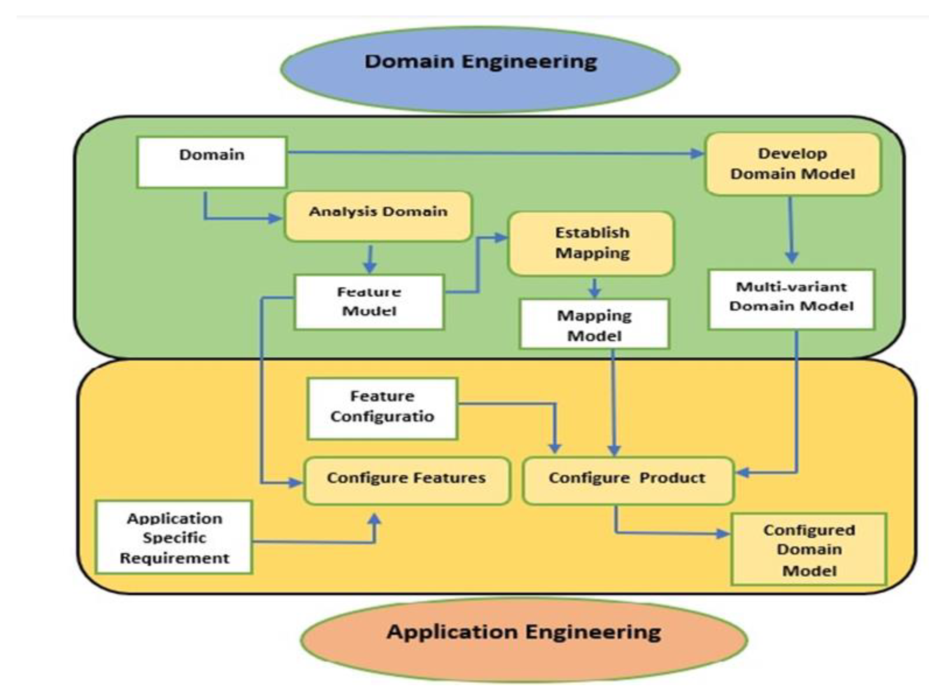
Figure 1. Software Product Line Engineering [5].
Preprints 76374 g001
Figure 2. Cell Phone Feature Model (adapted [45]).
Preprints 76374 g002
Figure 3. Individual Representation.
Preprints 76374 g003
Figure 4. Method Description.
Preprints 76374 g004
Figure 5. Non-Dominated Solutions Values for Different Feature Models.
Preprints 76374 g005
Figure 6. Counter Strike FM Pareto Fronts (Four Objectives) using Five MOEAs.
Preprints 76374 g006
Figure 7. Counter Strike FM Pareto Fronts Global (Four Objectives).
Preprints 76374 g007
Table 1. Feature Models Attributes.
Feature Model Features Configurations Number of Pairs
Counter Strike 24 18176 833
SPL SimulES, PnP 41 6912 2592
Smart Homev2.2 60 3.87×10⁹ 6189
Video Player 71 4.5×10¹³ 7528
Model Transformation 88 1.65×10¹³ 13139
Coche Ecologico 94 2.32×10⁷ 11075
Table 2. Parameters Settings.
Parameter Values
Population Size 200
Number of Generations 500
Crossover Rate 60%
Mutation Rate 30%
Table 3. Pareto Fronts with Four objectives Solutions.
Feature Models Algorithms
PFtrue IBEA MOEAD NSGAII NSGAIII SPEA2
PFcontribution
Counter Strike 465 13 (2.81%) 122 (26.23%) 24 (5.16%) 109 (23.44%) 197 (42.36%)
SPL SimulES, PnP 456 10 (2.19%) 138 (30.26%) 13 (2.85%) 97 (21.27%) 198 (43.42%)
Smart Home v2.2 499 8 (1.60%) 144 (28.85%) 23 (4.60%) 124 (24.84%) 200 (40.08%)
Video Player 456 8(1.75%) 124 (27.19%) 16 (3.5%) 108 (23.68%) 200 (43.85%)
Model Transformation 510 17 (3.4%) 141 (27.64%) 19 (3.72%) 133 (26.07%) 200 (39.21%)
Coche Ecologico 490 27 (5.51%) 123 (25.10%) 11 (2.24%) 129 (26.32%) 200 (40.81%)
Table 4. Indicators Hypervolume (HV) and Spacing Values for Four Objectives.
Indicator Feature Models IBEA MOEAD NSGAII NSGAIII SPEA2
Average St. D Average St. D Average St. D Average St. D Average St. D
HV Counter Strike 0.2826 0.1162 0.7094 0.0129 0.6029 0.0234 0.6498 0.0113 0.7022 0.0165
SPL SimulES, PnP 0.2698 0.0954 0.6524 0.0150 0.4659 0.0314 0.5413 0.0176 0.6390 0.0155
Smart Home v2.2 0.3460 0.1105 0.6885 0.0160 0.5742 0.0353 0.6052 0.0300 0.6843 0.0198
Video Player .0.3659 0.0969 0.6961 0.0155 0.5795 0.0108 0.6085 0.0262 0.6864 0.0193
Model Transformation 0.3600 0.0771 0.6009 0.0146 0.4677 0.0256 0.5276 0.0210 0.6136 0.0210
Coche Ecologico 0.3257 0.0802 0.4868 0.0048 0.3227 0.0107 0.4541 0.0329 0.5025 0.0013
Spacing Counter Strike 0.1138 0.0543 0.0329 0.0033 0.0496 0.0115 0.0316 0.0026 0.0157 0.0017
SPL SimulES, PnP 0.0713 0.0364 0.0208 0.0019 0.0521 0.0121 0.0295 0.0026 0.0113 0.0011
Smart Home v2.2 0.0753 0.0330 0.0302 0.0024 0.0474 0.0102 0.0342 0.0037 0.0126 0.0086
Video Player 0.0855 0.0430 0.0296 0.0028 0.0502 0.0108 0.0328 0.0046 0.0127 0.0015
Model Transformation 0.0527 0.0112 0.0262 0.0021 0.0412 0.0081 0.0292 0.0024 0.0102 0.0008
Coche Ecologico 0.0417 0.0173 0.0217 0.0016 0.0720 0.0218 0.0179 0.0030 0.0095 0.0013
Table 5. Fitness Values of Solutions with Objectives (O1, O2, O3, O4).
Feature Models Algorithms
IBEA MOEAD NSGAII NSGAIII SPEA2
Counter Strike O1(1,0.010,0.086,0.291)
O2(1,0.010,0.086,0.291)
O3(1,0.010,0.086,0.291)
O4(0.274, 0.030,0.365,1)
O1(1,0.010,0.623,0.666)
O2((1,0.010,0.623,0.666))
O3(1,0.010, 0.107, 0.291)
O4(0.271, 0.071, 0.136, 1)
O1(1,0.010,0.666, 0.75)
O2(1,0.010,0.666, 0.75)
O3(1,0.010, 0.107, .291)
O4(0.228, 0.051, .276,1)
O1(1,0.010,0.537,0.666)
O2(1,0.010,0.537,0.666)
O3(1,0.010,0.0107,0.291)
O4(0.238, 0.051, 0.219,1)
O1(1,0.010,0.709,0.791)
O2(1,0.010, 0.709,0.791)
O3(1,0.010,0.0107,0.291)
O4(0.260, 0.051, 0.198,1)
SPL SimulES, PnP O1(1,0.010,0.358,0.593)
O2(1,0.010, 0.358,0.593)
O3(1,0.010,0.305,0.05)
O4(0.625, 0.030,0.419,1)
O1(1,0.010,0.312,0.468)
O2(1,0.010, 0.312,0.468)
O3(1,0.010,0.229,0.50)
O4(0.638, 0.122,0.279,1)
O1(1,0.010,0.343,0.562)
O2(1,0.010, 0.343,0.562)
O3(1,0.010,0.236,0.50)
O4(0.654, 0.030,0.358,1)
O1(1,0.010,0.458,0.625)
O2(1,0.010, 0.458,0.625)
O3(1,0.010,0.244,0.468)
O4(0.669, 0.408,0.328,1)
O1(1,0.010,0.664,0.656)
O2(1,0.010, 0.664,0.656)
O3(1,0.010,0.236,0.50)
O4(0.647, 0.071,0.312,1)
Smart Home v2.2 O1(1,0.010,0.419,0.045)
O2(1,0.010, 0.419,0.045)
O3(1,0.010,0.257,0.366)
O4(0.264, 0.306,0.395,1)
O1(1,0.010,0.389,0.483)
O2(1,0.010, 0.389,0.483)
O3(1,0.010,0.069,0.20)
O4(0.161, 0.061,0.354,1)
O1(1,0.010,0.551,0.583)
O2(1,0.010, 0.551,0.583)
O3(1,0.010,0.077,0.216)
O4(0.178, 0.071,0.302,1)
O1(1,0.010,0.507,0.583)
O2(1,0.010, 0.507,0.583)
O3(1,0.010,0.036,0.133)
O4(0.190, 0.071,0.334,1)
O1(1,0.010,0.441,0.466)
O2(1,0.010, 0.441,0.466)
O3(1,0.010,0.106,0.216)
O4(0.239, 0.071,0.248,1)
Video Player O1(1,0.010,0.437,0.605)
O2(1,0.010, 0.437,0.605)
O3(1,0.010,0.234,0.450)
O4(0.128, 0.061,0.412,1)
O1(1,0.010,0.427,0.619)
O2(1,0.010, 0.427,0.619)
O3(1,0.010,0.128,0.352)
O4(0.174, 0.051,0.323,1)
O1(1,0.010,0.558,0.690)
O2(1,0.010, 0.558,0.690)
O3(0.801,0,0.156,0.521)
O4(0.206, 0.040,0.330,1)
O1(1,0.010,0.540,0.633)
O2(1,0.010, 0.540,0.633)
O3(0.772,0.010,0.161,0.535)
O4(0.279, 0.036,0.335,1)
O1(1,0.010,0.601,0.676)
O2(1,0.010, 0.601,0.676)
O3(1,0.010,0.163,0.380)
O4(0.214, 0.040,0.301,1)
Model Transformation O1(1,0.010,0.534,0.579)
O2(1,0.010, 0.534,0.579)
O3(1,0.010,0.193,0.363)
O4(0.211, 0.051,0.393,1)
O1(1,0.010,0.327,0.454)
O2(1,0.010, 0.327,0.454)
O3(1,0.010,0.161,0.318)
O4(0.021, 0.256,0.404,1)
O1(1,0.010,0.415,0.50)
O2(1,0.010, 0.415,0.50)
O3(1,0.010,0.170,0.340)
O4(0.165, 0.071,0.371,1)
O1(1,0.010,0.372,0.477)
O2(1,0.010, 0.372,0.477)
O3(1,0.010,0.170,0.284)
O4(0.224, 0.051,0.342,1)
O1(1,0.010,0.461,0.534)
O2(1,0.010, 0.461,0.534)
O3(1,0.010,0.179,0.284)
O4(0.158, 0.081,0.319,1)
Coche Ecologico O1(1,0.010,0.251,0.563)
O2(1,0.010, 0.251,0.563)
O3(1,0.010,0.202,0.563)
O4(0.143, 0.112,0.268,1)
O1(1,0.010,0.398,0.659)
O2(1,0.010, 0.398,0.659)
O3(1,0.010,0.156,0.510)
O4(0.180, 0.816,0.251,1)
O1(1,0.010,0.310,0.574)
O2(1,0.010, 0.310,0.574)
O3(1,0.010,0.156,0.521)
O4(0.094, 0.173,0.275,1)
O1(1,0.010,0.310,0.574)
O2(1,0.010, 0.310,0.574)
O3(1,0.010,0.156,0.521)
O4(0.094, 0.173,0.275,1)
O1(1,0.010,0.316,0.617)
O2(1,0.010, 0.316,0.617)
O3(1,0.010,0.156,0.50)
O4(0.149, 0.102,0.255,1)
Table 6. Better MOEA Algorithm with respect to Indicators (HV and Spacing).
Feature Models Quality Indicators
Hyper Volume Spacing
Counter Strike MOEA/D, SPEA2, NSGAIII MOEA/D, SPEA2, NSGAIII
SPL SimulES, PnP MOEA/D, SPEA2 MOEA/D, SPEA2, NSGAIII
Smart Home v2.2 MOEA/D, SPEA2, NSGAIII MOEA/D, SPEA2, NSGAIII
Video Player MOEA/D, SPEA2, NSGAIII MOEA/D, SPEA2
Model Transformation MOEA/D, SPEA2, NSGAIII MOEA/D, SPEA2, NSGAIII
Coche Ecologico MOEA/D, SPEA2, NSGAIII SPEA2, NSGAIII,
Disclaimer/Publisher’s Note: The statements, opinions and data contained in all publications are solely those of the individual author(s) and contributor(s) and not of MDPI and/or the editor(s). MDPI and/or the editor(s) disclaim responsibility for any injury to people or property resulting from any ideas, methods, instructions or products referred to in the content.
Copyright: This open access article is published under a Creative Commons CC BY 4.0 license, which permit the free download, distribution, and reuse, provided that the author and preprint are cited in any reuse.
Prerpints.org logo

Preprints.org is a free preprint server supported by MDPI in Basel, Switzerland.

Subscribe

© 2024 MDPI (Basel, Switzerland) unless otherwise stated