Preprint
Article

RL-Based Detection, Tracking, and Classification of Malicious UAV Swarm through Airborne Cognitive Multibeam Multifunction Phased Array Radar

Altmetrics

Downloads

140

Views

79

Comments

0

A peer-reviewed article of this preprint also exists.

This version is not peer-reviewed

Submitted:

13 June 2023

Posted:

13 June 2023

You are already at the latest version

Alerts
Abstract
Detecting, tracking, and classifying unmanned aerial vehicles (UAVs) in a swarm presents significant challenges due to their small and diverse radar cross-sections, multiple flight altitudes, velocities, and close trajectories. To overcome these challenges, adjustments of the radar parameters and/or position of the radar (for airborne platforms) are often required during runtime. The runtime adjustments help to overcome the anomalies in the detection, tracking, and classification of UAVs. The runtime adjustments are performed either manually or through fixed algorithms, each of which can have its limitations for complex and dynamic scenarios. In this work, we propose the use of multi-agent reinforcement learning (RL) to carry out the runtime adjustment of the radar parameters and position of the radar platform. The radar used in our work is a multibeam multifunction phased array radar (MMPAR) placed onboard UAVs. The simulations show the cognitive adjustment of the MMPAR parameters and position of the airborne platform using RL helps to overcome anomalies in the detection, tracking, and classification of UAVs in a swarm. A comparison with other artificial intelligence (AI) algorithms shows that RL performs better due to runtime learning of the environment through rewards.
Keywords: 
Subject: Engineering  -   Electrical and Electronic Engineering

1. Introduction

Unmanned aerial vehicles (UAVs), commonly referred to as drones, have gained tremendous popularity over the past decade [1,2]. Nowadays, UAVs are used in numerous applications [3,4] and their usage is expected to increase in the future [5]. However, UAVs can also be exploited for malicious purposes, posing significant threats [6]. The main reason behind these threats is the limitations in early detection, tracking, and classification of malicious UAVs at long ranges due to their small radar cross-section (RCS) and their ability to fly close to the terrain [6]. Additionally, the challenges of detecting, tracking, and classifying UAVs are heightened when they fly in a swarm, as these UAVs can have varying RCS, velocities, and follow complex, time-varying trajectories in close proximity to each other.
Numerous research efforts are underway to develop novel methods for UAV detection, tracking, and classification [7]. Detection methods can be broadly classified into two categories: non-radar-based and radar systems [6]. Popular non-radar based methods include electro-optical/infrared, radio frequency (RF) analysis, and analysis of sound emissions from the UAV [6,8]. The majority of the non-radar systems have no active emissions. The passive detection of UAVs using non-radar systems have limitations discussed in [6]. Compared to non-radar methods, radar-based methods are popular and widely used for the detection, tracking, and classification of UAVs. Radar-based methods can be further classified into conventional and non-conventional methods. Conventional radar systems are monostatic and rely on active RF transmissions, but they have limitations in detecting and tracking small UAVs due to their small RCS and ability to fly close to clutter [6,9]. Non-conventional radar systems, on the other hand, can detect and track small UAVs, although their operation is often restricted to specific types of UAVs and environmental scenarios. Popular non-conventional radar systems for UAV detection, tracking, and classification include micro-Doppler radars, phase-interferometric radars, multistatic radars, and passive radars [10,11,12,13].
Cognitive radars, another non-conventional radar system, are capable of outperforming conventional radar systems in complex and dynamic scenarios [14]. Cognitive radars provide a high level of situational awareness by continuously monitoring the environment and adjusting the radar parameters accordingly [15]. Cognitive radars are also able to support autonomous operations and are less reliant on input from human operators. Additionally, cognitive radars can use various artificial intelligence (AI) algorithms for optimal parameter adjustments based on the situation at hand. For example, in [16], a non-linear transformation-based machine learning approach is used for adaptively adjusting the detection threshold. In [17], different aspects of cognition implemented through neural networks are discussed. Reinforcement learning (RL) is also a popular method to introduce cognition into radar systems. In [18], deep RL is used for optimal radar performance by varying the bandwidth and center frequency in spectrally congested environments.
In this work, we present the implementation of a network of airborne UAVs equipped with a multibeam multifunction phased array radar (MMPAR) for the detection, tracking, and classification of malicious UAVs in a swarm. The multifunction beams used in our work are shown in Figure 1. The parameters of the MMPAR and the position of the UAV carrying MMPAR are controlled cognitively through the multi-agent RL algorithm. Multiple airborne MMPAR onboard UAVs are used to detect, track, and classify malicious UAVs in a swarm. The anomalies during the detection, tracking, and classification of UAVs in a swarm are identified and optimum actions are taken to remove the anomalies. The optimum actions are based on the highest Q-values to remove corresponding anomalies. We compare our RL approach with other AI algorithms and show that RL handles the anomalies better due to its runtime feedback from the environment in the form of rewards. Additionally, when no target is detected, the MMPAR onboard UAV can serve as a communication relay, providing communication to ground nodes. Overall, our approach provides the following advantages:
  • Common UAVs cannot carry a large multifunction radar due to weight and power constraints. To overcome this limitation, we propose an approach that employs multiple small MMPARs carried by UAVs. These radar nodes are networked to provide a cumulative radar response, allowing us to detect, track, and classify malicious UAVs in a swarm.
  • By using multiple MMPAR nodes, our approach eliminates the risk of a single-point failure due to malfunction or external jamming.
  • Using multiple MMPAR nodes onboard UAVs provides superior spatial coverage and mobility compared to a single radar node on the ground.
  • The use of multiple radar beams in MMPAR and the ability to adaptively schedule the beams help to accurately resolve multiple targets in range, Doppler, and angular domains. This is because the multiple beams provide better spatial coverage and resolution, while adaptive scheduling ensures that the beams are directed towards areas of interest, where potential targets may be present. Additionally, the use of multiple beams also helps to mitigate the effects of clutter and interference, which can degrade radar performance.
  • The multifunction beams generated by the MMPAR can be used for other tasks in addition to the main radar task. For example, the beams can be used for communication purposes or for RF passive listening, which can be performed simultaneously by sharing the radar resources adaptively. This allows for efficient utilization of the MMPAR resources, enabling the UAVs to perform multiple tasks with a single device.
  • Anomaly detection and removal is an important aspect of our approach, as it helps to reduce false alarms and improve the accuracy of the system. By using RL, the system is able to learn from its environment and adjust its parameters to improve its performance. This can help to identify and remove anomalies in real-time, leading to more reliable and efficient detection, tracking, and classification of UAVs.
  • Our approach works optimally in complex and dynamically changing scenarios, e.g., UAV swarms, clutter, and jamming.
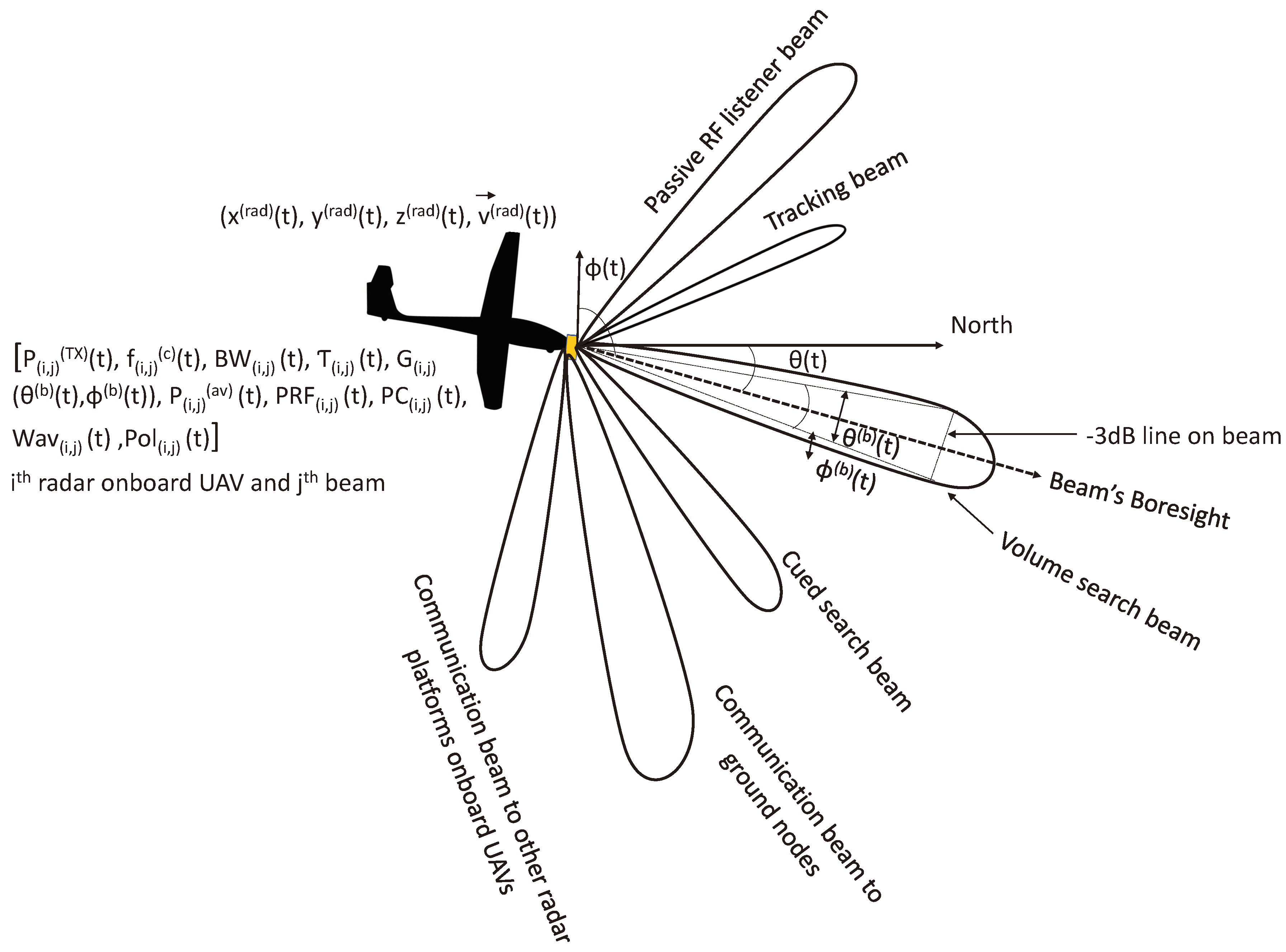
Figure 1. Six multifunction beams j = 1 , 2 , , 6 , originating from an i th MMPAR onboard a UAV. The parameters of all beams are different.
Preprints 76460 g001
To the best of our knowledge, MMPAR using multi-agent RL to detect, track, and classify UAVs in a swarm is not available in the literature. A comparison of our work with corresponding literature is provided in Table 1. The rest of the paper is organized as follows: Section 2 provides the details of the MMPAR setup onboard UAV, multi-agent RL used in our work is given in Section 3, simulation setup and results are provided in Section 4, and Section 5 concludes the paper.

2. Multibeam Multifunction Phased Array Radar onboard UAVs

In this section, beam steering and scheduling of MMPAR are discussed. The details of MMPAR and target parameters are also provided in this section.

2.1. Steering and Scheduling of Multifunction Phased Array Beams

In our approach, we consider that there is an N UAVs, each of which carries an MMPAR. The MMPAR on multiple UAVs are networked through communication beams. Each MMPAR has a B steerable phased array beams. Each beam performs a given function. The radiation pattern of the j th beam, for j = 1 , 2 , , B is given as F j θ , ϕ = F j ( arr ) ( θ , ϕ ) × F ( ant ) ( θ , ϕ ) , where F j θ , ϕ is the overall radiation pattern of the j th beam, and θ , and ϕ represent the angles in the azimuth and elevation planes, respectively, F j ( arr ) and F ( ant ) are the array factor of the j th beam and antenna radiation pattern of individual elements of the array, respectively. Each j th beam is steerable in the range [ θ j ( lim ) : Δ θ : θ j ( lim ) ] and [ ϕ j ( lim ) : Δ ϕ : ϕ j ( lim ) ] , where, θ j ( lim ) and ϕ j ( lim ) are the scanning limits of the beam in the azimuth and elevation planes, respectively, and | θ j ( lim ) | > | ϕ j ( lim ) | j . The angular step between any two steering angles in the azimuth and elevation planes is represented as Δ θ and Δ ϕ , respectively.
Our approach uses six beams, as shown in Figure 1, denoted by B = 6 . These beams include two communication beams, a volume search beam, a cued search beam, a track beam, and a passive RF listener beam. Each beam has unique characteristics that depend on its function. For instance, the half-power beamwidth of the communication, volume search, and passive RF listener beams are larger compared to the cued search beam. The track beam has the highest angular resolution and gain, and is used to estimate the final parameters of the target. Although the large beamwidths of the volume search, communication, and passive RF listener beams allow for large spatial area coverage during a scan, the angular resolution is relatively small. Furthermore, to maintain simplicity, we have taken the steering limits of the beams to be the same in both the azimuth and elevation planes.
Algorithm 1 outlines the working of the MMPAR and beam scheduling. The six beams are scheduled adaptively based on the detected targets. At the beginning of the update interval δ t , beam scheduling requests are received. The scheduling of beams for the duration δ t is determined based on the received requests, the current state of the beams, the target state, and the priority sequence. The details of functions performed and the scheduling of beams are as follows:
  • There are two communication beams as shown in Figure 1 and Figure 2. One communication beam facilitates communication between the UAVs and is always available with the highest scheduling priority. The other communication beam forms a link between the ground station (GS) and the MMPAR on board the UAV, allowing the MMPAR to function as a communication relay. Both communication beams and the volume search beam operate simultaneously during a given δ t . However, when a target is detected by the volume search beam, the second communication beam ceases operation, and communications from the second beam are transferred to other GS nodes.
  • To improve the detection and tracking of UAVs, the volume search beam is designed with the largest coverage among all the beams. This enables the radar to scan a vast volume of space during the given time interval δ t . However, once a target is detected, the scheduling priority of the volume search beam corresponding to that target is reduced for future update intervals. This approach ensures that the other beams with higher scheduling priority can focus on tracking the target with more accuracy and efficiency.
  • The cued search beam is used to confirm the presence of a target detected by the volume search. Both the cued search and volume search beams can scan simultaneously.
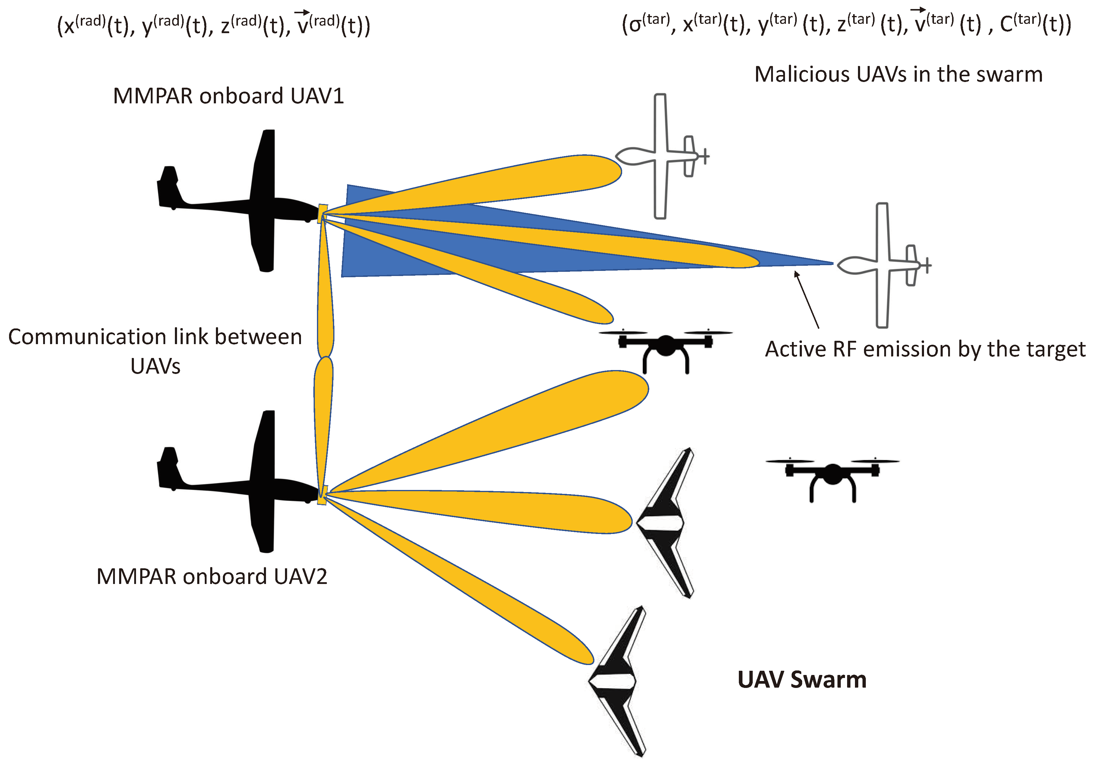
  • The tracking beam is directed towards the coordinates provided by the cued search beam after a time interval of δ t . As the coverage area of the track beam is significantly larger than the physical tracks covered by a target during δ t , the target remains within the coverage area. Due to its high angular and range resolution, the tracking beam can distinguish between multiple targets in the range and angular bins, and estimate their position, RCS, and Doppler estimates. Additionally, the tracking beam has a higher priority (after confirming target presence) than other beams. Targets are tracked adaptively, meaning that mobile/fast-moving targets are visited frequently compared to static/slow targets to update their state. Figure 3 illustrates the interaction of different types of beams with targets.
  • The passive RF listener beam is not scheduled in a fixed sequence but rather randomly applied at different time intervals of δ t . Its purpose is to detect active RF emissions from a malicious UAV, including intentional RF emissions for jamming and the RF link of the UAV for further analysis. Figure 3 illustrates the passive RF listener beam that is used to detect directed RF emissions from a malicious UAV.
Algorithm 1 Pseudo-code for beam scheduler and working of MMPAR.
  1:
procedure  RadarBeamScheduler
  2:
% Beam scheduling and radar operation.
  3:
% i = 1 , 2 , , N are the number of MMPAR, each onboard a UAV.
  4:
% Input to the procedure are the MMPAR beams and corresponding resources: S i , j ( rad ) ( t ) , i , j = 1 , 2 , , 6 , given in (2).
  5:
At the start of every update interval δ t :
  6:
RF passive listener beam applied if r a n d > 0.5 , where r a n d is a random generator in the range [ 0 1 ) .
  7:
    if No target is detected then
  8:
        Volume search and communication beams continue during δ t .
  9:
    end if
10:
    if a target is detected then
11:
        Request the handover of current relay-based communications to the GS nodes.
12:
        Store the coordinates of the target during the current volume search as x ( tar , vol ) ( t ) , y ( tar , vol ) ( t ) , z ( tar , vol ) ( t ) .
13:
        At the same δ t , direct the cued search beam toward the coordinates of the target obtained during volume search.
14:
        if cued search confirms the target then
15:
           Store the coordinates of the target as x ( tar , cue ) ( t ) , y ( tar , cue ) ( t ) , z ( tar , cue ) ( t ) .
16:
           At the next update interval t + δ t , direct the track beam toward the estimated position of the target obtained from the cued search. The coordinates of the target after applying the track beam are estimated as x ( tar , trk ) ( t + δ t ) , y ( tar , trk ) ( t + δ t ) , z ( tar , trk ) ( t + δ t ) . The RCS and Doppler estimates of the target are also obtained.
17:
           At every next update interval (provided the target is present in the previous interval) the track beam will be assigned the highest priority. The state of the target S i ( tar ) is updated at every δ t .
18:
           Also, the targets are tracked adaptively, i.e., targets with high maneuverability are visited often compared to slow-moving targets.
19:
        else
20:
           Confirm targets again using volume search.
21:
        end if
22:
    else
23:
        Continue using communication and search beams.
24:
    end if
25:
    During all δ t , the communications between the MMPAR onboard UAVs continue.
26:
return The target state, S i ( tar ) .
27:
end procedure
Figure 2. The UAV carrying the MMPAR moves in a straight line at a constant velocity. MMPAR emits volume search and communication beams when no target is detected. Once a target is detected, the communication link with ground nodes is handed over to other ground communication nodes.
Preprints 76460 g002
Figure 3. Two UAVs equipped with MMPAR are utilized to detect malicious UAVs operating as a swarm. The multifunction beams of MMPAR are employed for searching, tracking, passive listening (for active RF emissions), and classifying targets. However, one of the malicious UAVs in the swarm is causing interference with its active RF emissions. Additionally, one of the beams is utilized for communication between the radar platforms.
Preprints 76460 g003

2.2. MMPAR Parameters

The radar parameters assigned to each type of beam are unique. The configurable radar and radar platform parameters are provided in Table 2. The range of radar parameters provided in the Table 2 can be represented as
P ( TX ) = P ( TX , max ) : Δ P ( TX ) : P ( TX , min ) , f ( c ) = f ( c , max ) : Δ f ( c ) : f ( c , min ) , B W = B W ( max ) : Δ B W : B W ( min ) , τ = τ ( max ) : Δ τ : τ ( min ) , θ ( b ) = θ ( b , max ) : Δ θ ( b ) : θ ( b , min ) , ϕ ( b ) = ϕ ( b , max ) : Δ ϕ ( b ) : ϕ ( b , min ) , P R F = P R F ( max ) : Δ P R F : P R F ( min ) , P C = P C k , k = 1 , 2 , , N ( PC ) , W a v = W a v k , k = 1 , 2 , , N ( Wav ) , P o l = P o l k , k = 1 , 2 , , N ( Pol ) ,
where, P ( TX , max ) , P ( TX , min ) are the maximum and minimum transmit power, respectively, and Δ P ( TX ) represents the step change in the transmit power, f ( c , max ) and f ( c , min ) is the maximum and minimum center frequency, respectively, and Δ f ( c ) is the step change in the center frequency. The maximum and minimum bandwidth ranges are represented by B W ( max ) , and B W ( min ) , respectively, and Δ B W is the step change in the bandwidth, τ ( max ) , and τ ( min ) are the maximum and minimum pulsewidths, respectively, and Δ τ is the step change between the pulsewidth values, the maximum and minimum azimuth half-power beamwidths are represented as θ ( b , max ) and θ ( b , min ) , respectively, and Δ θ ( b ) is the step change of the beamwidth in the azimuth plane, and ϕ ( b , max ) , ϕ ( b , min ) are the maximum and minimum half-power beamwidths in the elevation plane, and Δ ϕ ( b ) is the step change of the beamwidth in the elevation plane. The maximum and minimum range of the PRF is represented as P R F ( max ) and P R F ( min ) , respectively, and Δ P R F is the step change in the PRF, N ( PC ) is the number of intrapulse modulation options available, N ( Wav ) is the number of waveform types available, and N ( Pol ) is the number of polarization options available. Moreover, the range of (the magnitude of) the velocity of an i th airborne radar platform (UAV) is given as v i ( rad , max ) : v i ( rad , min ) .
Different types of beams are assigned different radar parameters from (1). The parameters assigned to simultaneously scheduled beams should be smaller than or equal to the total resources of the parameters available. The parameters assigned to beams remain the same unless a change is recommended by the cognitive block. Let S ( i , j ) ( rad ) ( t ) represent the j th beam at the i th radar onboard UAV at time t. The beam S ( i , j ) ( rad ) ( t ) and the corresponding radar parameters assigned are given as
S ( i , j ) ( rad ) ( t ) = [ P ( i , j ) ( TX ) ( t ) f ( i , j ) ( c ) ( t ) B W ( i , j ) ( t ) τ ( i , j ) ( t ) G ( i , j ) θ ( b ) ( t ) , ϕ ( b ) ( t ) P ( i , j ) ( av ) ( t ) P R F ( i , j ) ( t ) P C ( i , j ) ( t )
W a v ( i , j ) ( t ) P o l ( i , j ) ( t ) ] .
Table 2. Radar and radar platform parameters.
Serial # Radar parameter Representation
1 Transmit power P ( TX )
2 Center frequency f ( c )
3 Bandwidth B W
4 Pulsewidth τ
5 Antenna gain based on beamwidths
in the azimuth and elevation planes
G θ ( b ) , ϕ ( b )
6 Pulse repetition frequency P R F
7 Power aperture product,
(where A θ ( b ) , ϕ ( b ) is the subarray aperture size)
P ( av ) = P ( TX , max ) τ P R F A θ ( b ) , ϕ ( b )
8 Intrapulse modulation/pulse compression P C
9 Waveform type W a v
10 Polarization P o l
11 Radar platform position ( x ( rad ) , y ( rad ) , z ( rad ) )
12 Radar platform velocity v ( rad )

3. Reinforcement Learning in our Approach

In this section, we first discuss the states of the targets, followed by a discussion of anomalies in the detection, tracking, and classification of targets. We then present the implementation of multiagent Q-learning to remove these anomalies. Additionally, we discuss the implementation of supervised AI algorithms for the same purpose.

3.1. State of the Targets

We consider that there are M malicious UAVs (taken as targets) in the swarm. Each MMPAR onboard a UAV detects a subset of the total targets given as k = 1 , 2 , , M i . The RCS, position, and velocity estimates (based on Doppler), of the k th target detected by i th MMPAR is represented as ρ ( i , k ) ( tar ) , ( x ( i , k ) ( tar ) , y ( i , k ) ( tar ) , z ( i , k ) ( tar ) ), and v ( i , k ) ( tar ) , respectively. Classification is performed by assigning a class category C ( i , k ) ( tar ) to each target based on its RCS and velocity. For simplification, we defined two class categories. One class category is the fixed wing and the other is the rotary wing.
Moreover, each k th target is detected at a given signal-to-noise ratio (SNR) on i t h MMPAR represented as S N R ( k , i ) ( tar ) . The SNR for the search, cued, track, and passive listening beams are given, respectively, as
S N R ( k , i , j ) ( sr , tar ) = P ( i , j ) ( av ) t ( i , j ) ( s ) σ ( k , i ) 4 π Ω ( i , j ) R ( k , i ) 4 k T i ( s ) L i , j = 3 ,
S N R ( k , i , j ) ( cue , tar ) = P ( i , j ) ( TX , max ) G 2 θ ( i , j ) ( b ) , ϕ ( i , j ) ( b ) λ i 2 σ ( k , i ) ( 4 π ) 3 R ( k , i ) 4 k T i ( s ) B i ( n ) L i , j = 4 ,
S N R ( k , i , j ) ( trk , tar ) = P ( i , j ) ( TX , max ) G 2 θ ( i , j ) ( b ) , ϕ ( i , j ) ( b ) λ i 2 σ ( k , i ) ( 4 π ) 3 R ( k , i ) 4 k T i ( s ) B i ( n ) L i , j = 5 ,
S N R ( k , i , j ) ( pl , tar ) = E I R P ( tar ) G θ ( i , j ) ( b ) , ϕ ( i , j ) ( b ) λ i 2 4 π R ( k , i ) 2 k T i ( s ) B i ( n ) L i , j = 6 ,
where t ( i , j ) ( s ) and Ω ( i , j ) is the scan time and solid angle, respectively, for the volume search beam ( j = 3 ) at i th radar, T i ( s ) , L i , and B i ( n ) represent the system temperature, cumulative losses, and noise bandwidth of the radar receiver, respectively, at the i th radar, k is the Boltzman constant, R is the range of the target, and E I R P ( tar ) is the effective isotropic radiated power (EIRP) emitted by the active RF emitter onboard a target.
The RCS, position, velocity, class category, and detected SNR (obtained during tracking and passive listening) are considered as state of the target. The current state of the targets (numbered as k = 1 , 2 , , M i ) observed at i th UAV are given as
S i ( tar ) ( t ) = ρ ( i , 1 ) ( tar ) ( t ) x i , 1 ( tar ) ( t ) y ( i , 1 ) ( tar ) ( t ) z ( i , 1 ) ( tar ) ( t ) ρ ( i , 2 ) ( tar ) ( t ) x i , 2 ( tar ) ( t ) y ( i , 2 ) ( tar ) ( t ) z ( i , 2 ) ( tar ) ( t ) ρ ( i , M i ) ( tar ) ( t ) x i , M i ( tar ) ( t ) y ( i , M i ) ( tar ) ( t ) z ( i , M i ) ( tar ) ( t ) v ( i , 1 ) ( tar ) ( t ) C ( i , 1 ) ( tar ) ( t ) S N R ( i , 1 ) ( trk , tar ) ( t ) v ( i , 2 ) ( tar ) ( t ) C ( i , 2 ) ( tar ) ( t ) S N R ( i , 2 ) ( trk , tar ) ( t ) v ( i , M i ) ( tar ) ( t ) C ( i , M i ) ( tar ) ( t ) S N R ( i , M i ) ( trk , tar ) ( t ) .
Similarly, the past states of the targets over n δ t observation intervals stored in corresponding arrays are given as
S i ( tar ) ( t δ t : t n δ t ) = ρ ( i , 1 ) ( tar ) x ( i , 1 ) ( tar ) y ( i , 1 ) ( tar ) z ( i , 1 ) ( tar ) ρ ( i , 2 ) ( tar ) x ( i , 2 ) ( tar ) y ( i , 2 ) ( tar ) z ( i , 2 ) ( tar ) ρ ( i , M i ) ( tar ) x ( i , M i ) ( tar ) y ( i , M i ) ( tar ) z ( i , M i ) ( tar ) v ( i , 1 ) ( tar ) C ( i , 1 ) ( tar ) SNR ( i , 1 ) ( trk , tar ) v ( i , 2 ) ( tar ) C ( i , 2 ) ( tar ) SNR ( i , 2 ) ( trk , tar ) v ( i , M i ) ( tar ) C ( i , M i ) ( tar ) SNR ( i , M i ) ( trk , tar ) .
Both the current and past states of the targets over n δ t update time intervals are provided to the RL cognitive block shown in Figure 4.

3.2. Anomalies

An anomaly can be defined as a random fluctuation in the state of a target, which can be caused by external factors such as clutter and RF interference in the environment, or by limitations in radar processing. Such limitations include range and Doppler ambiguities, range resolution, angular resolution, radar receiver sensitivity, and dynamic range. Anomalies are expected to increase in complex and dynamic scenarios, such as those involving time-varying clutter and UAV swarms. These anomalies can result in inaccurate detection, tracking, and classification of targets. At a given time t, anomaly in the state of a k th target observed at i th MMPAR can be represented as
ρ ( i , k ) ( tar ) ( t ) = ρ ( i , k ) ( tar ) ( t ) + X ( rcs ) ( t ) , x ( i , k ) ( tar ) ( t ) = x ( i , k ) ( tar ) ( t ) + X ( pos ) ( t ) , y ( i , k ) ( tar ) ( t ) = y ( i , k ) ( tar ) ( t ) + X ( pos ) ( t ) , z ( i , k ) ( tar ) ( t ) = z ( i , k ) ( tar ) ( t ) + X ( pos ) ( t ) , v ( i , k ) ( tar ) = v ( i , k ) ( tar ) + X ( v ) ( t ) , C ( i , k ) ( tar ) ( t ) = C ( i , k ) ( tar ) ( t ) + X ( C ) ( t ) , S N R ( i , k ) ( tar ) ( t ) = S N R ( i , k ) ( tar ) ( t ) + X ( SNR ) ( t ) ,
where ρ ( i , k ) ( tar ) ( t ) , x ( i , k ) ( tar ) ( t ) , y ( i , k ) ( tar ) ( t ) , z ( i , k ) ( tar ) ( t ) , v ( i , k ) ( tar ) , C ( i , k ) ( tar ) ( t ) , and S N R ( i , k ) ( tar ) ( t ) represent the target state with anomalies due to random fluctuations, and X ( rcs ) ( t ) , X ( pos ) ( t ) , X ( v ) ( t ) , X ( C ) ( t ) , X ( SNR ) ( t ) are the random processes for RCS, position, velocity, classification, and SNR, respectively.
An anomaly detector is used to identify anomalies during radar processing. In Figure 4, an anomaly detector for i th MMPAR onboard a UAV is shown. The inputs to the anomaly detector are the present and past states of the targets, S i ( tar ) ( t ) and S i ( tar ) ( t δ t : t n δ t ) , respectively (provided in Section 3.1). The anomaly detector in Figure 4 also contains a policy and an anomaly classifier block corresponding to a given terrain. An anomaly is identified by comparing the current and past states of a target over duration n δ t with a given policy. The anomaly detection procedure is described in Algorithm 2. A list of the possible anomalies during the detection, tracking, and classification of UAVs in a swarm is provided in Table 3.

3.3. Multi-agent Q-Learning

If an anomaly persists for a duration of n δ t , then corrective action is required to remove the anomaly. Such corrective action involves changing the runtime radar parameters and/or repositioning the radar platform. Table 4 provides a list of possible actions to remove the anomalies listed in Table 3. The combined set of available actions A i ( t ) at a given time t and at the i th MMPAR can be represented as
A i ( t ) = S i ( rad ) ( t ) x ( rad ) , y ( rad ) , z ( rad ) .
Choosing an action from Table 4 may not result in an optimal outcome. It is preferable to select an action that can maximize current and future returns, i.e., remove current and potential future anomalies with minimum overhead. After an action is taken, we can reach three states given in Table 5. Each state has an associated fixed reward. There is also an overhead for each action represented by O. The total reward is the addition of a fixed reward for the state action pair and overhead for the action shown in Table 5. This reward is used to calculate the Q-value given in Algorithm 2. The optimum Q-values are obtained after multiple iterations of training. Overall, the anomalies, corresponding optimum actions, and Q-values are listed in Table 6.
Algorithm 2 Pseudo-code for multi-agent RL algorithm using Q-learning and MMPAR data.
  1:
procedure  StateAnomalyActionReward
  2:
% The input to the algorithm are target states S ( tar ) ( t ) , radar parameters S ( rad ) ( t ) , radar platform position ( x ( rad ) , y ( rad ) , z ( rad ) ), and policy for a given scenario.
  3:
    Consider that we are at i th MMPAR onboard a UAV.
  4:
    if  S i ( tar ) ( t ) and S i ( tar ) ( t δ t : t n δ t ) do not conform to the policy for anomaly then
  5:
        Identify the anomaly.
  6:
        if Anomaly is already present in the anomaly list then
  7:
           For a k th anomaly, p th state, reward r, and j th action from Table 5, the corresponding Q-value is calculated as:
  8:
            New Q S i , k , p ( tar ) ( t ) , a i , k , p , j ( t ) = Q S i , k , p ( tar ) ( t ) , a i , k , p , j ( t ) + β [ r i , k , p , j ( t ) S i , k , p ( tar ) ( t ) , a i , k , p , j ( t ) + γ maxQ S i , k , p ( tar ) ( t ) , a i , k , p , j ( t ) Q S i , k , p ( tar ) ( t ) , a i , k , p , j ( t ) ]     % where β is the learning rate, r is the reward, γ is the future discount rate, and Q represents maximum expected future rewards given a future state S , and action a .
  9:
           Update the Q-learning table.
10:
        else
11:
           Update the anomaly list.
12:
        end if
13:
    end if
14:
return Q-learning table given in Table 6.
15:
end procedure
Algorithm 3 Pseudo-code for evaluation and comparison of RL-based approach with other AI algorithms.
  1:
procedure  Evaluation-RL-AI
  2:
% For RL evaluation
  3:
    Create a dynamically changing scenario by introducing multiple targets and randomness representing noise and clutter, and active RF interference emissions.
  4:
    Identify anomalies and select optimum action based on Q-value. See Table 6.
  5:
    if Anomaly persists after an optimum action then
  6:
        Take the action with lesser priority (smaller Q-value than the previous).
  7:
        if Anomaly is removed after lesser priority action then
  8:
           Update the Q-learning table with an updated Q-value for the new action.
  9:
        else
10:
           Select another action with a lower priority and repeat.
11:
        end if
12:
    end if
13:
    Calculate the percentage of recurrence of anomalies after corrective actions are applied.
14:
% For supervised AI algorithms
15:
    For an anomaly, the AI algorithm is trained with an optimum action label based on the target state S i ( tar ) ( t ) and radar parameters S i ( rad ) ( t ) .
16:
    Calculate the percentage of recurrence of anomalies for different supervised AI algorithms.
17:
return Percentage recurrence of anomalies for RL and supervised AI algorithms.
18:
end procedure
Algorithm 2 provides the implementation of multi-agent Q-learning using MMPAR data. Each MMPAR onboard a UAV acts as an RL agent. The state of each agent is represented by the current and previous states of the targets after an anomaly is detected. Q-values are learned using the Q-learning algorithm and rewards from the environment for a given state-action pair. The optimum action based on Q-value is updated in Table 6. To evaluate the Q-learning table in a simulated environment scenario, multiple targets, noise, clutter, and active RF emissions as interference are introduced to create a complex and dynamic scenario. Algorithm 3 outlines the evaluation procedure.
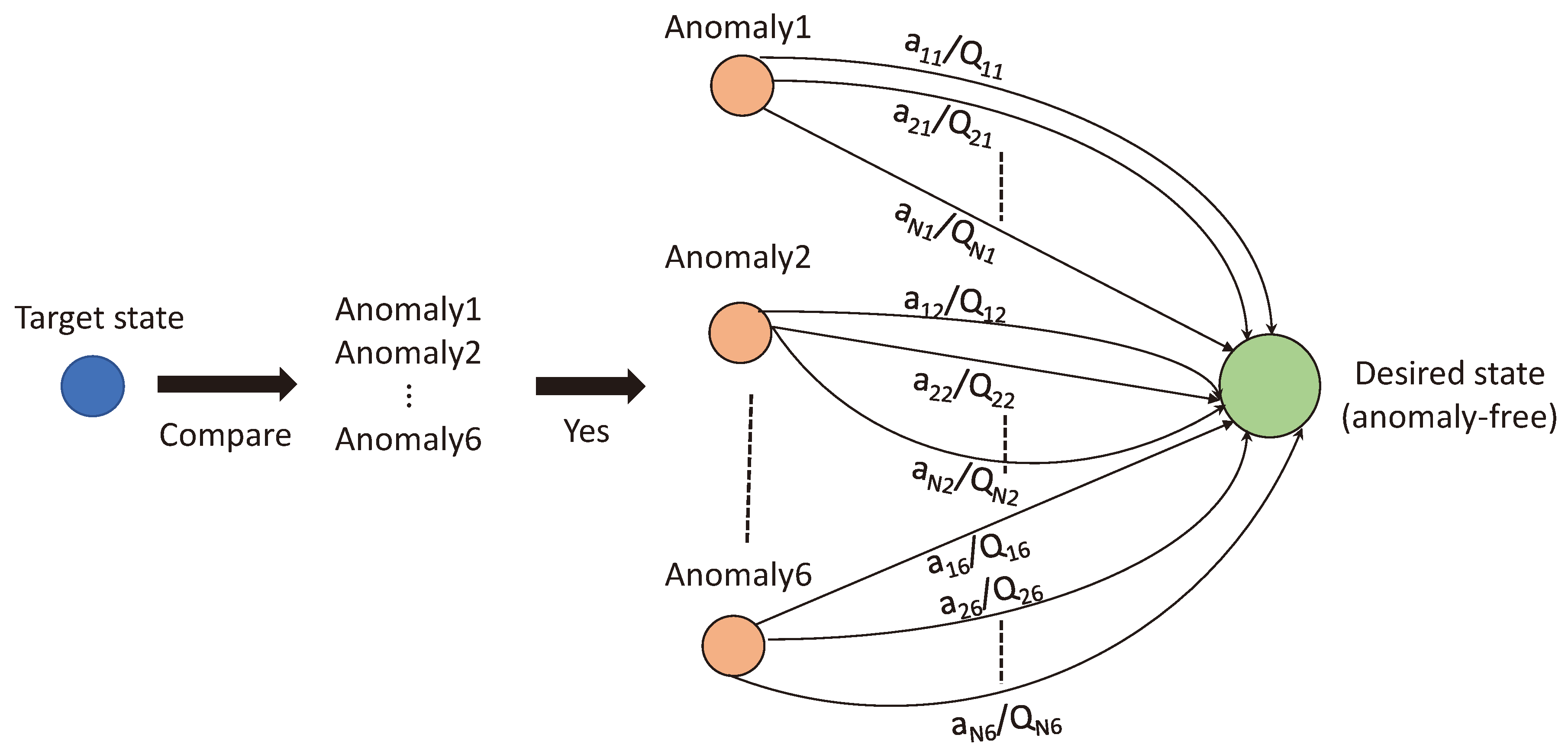
A Markov decision process (MDP) is a mathematical framework used to model decision-making problems in situations where outcomes are partly random and partly under the control of a decision maker. In the case of the presented approach, the MDP represents the states of the targets, the occurrence of anomalies, the actions taken to remove the anomalies, and the corresponding Q-values shown in Figure 5.
Table 4. Possible actions to eliminate anomalies for accurate detection, tracking, and classification of UAVs in the swarm.
Serial # Action Action label
1 Change of center frequency a 1
2 Change of pulsewidth a 2
3 Change of bandwith a 3
4 Change of PRF a 4
5 Introduce intrapulse modulation or change of type of intrapulse modulation a 5
6 Change of number of pulses a 6
7 Change in transmit power a 7
8 Change of antenna beamwidth a 8
9 Change in the polarization of the phased array a 9
10 Change in type of sounding signal a 10
11 Changes in the beam scheduling a 11
12 Change of position of the radar platform onboard UAV a 12
Figure 5. A Markov decision process is used to represent our approach. Initially, the state of the target is examined for anomalies at a particular radar onboard UAV. If an anomaly is detected, a set of actions is available to correct the anomaly and transition to the desired state. Each action corresponds to a Q-value. The action with the highest Q-value is selected.
Preprints 76460 g005
The goal of the MDP is to achieve an anomaly-free state for radar operation. If an anomaly arises, the best action is chosen based on the optimum Q-value to remove the anomaly and move to the desired state as shown in Figure 5. If the action based on an optimum Q-value is not able to remove the anomaly, the Q-value is updated for the state-action pair using a negative reward. A second priority action is used to remove the anomaly if the first action fails, and the process repeats. By using an MDP, the approach can systematically and optimally address anomalies in radar operation.
Table 5. There are six anomalies identified in our approach. Three states can arise after an anomaly occurs and an action is taken. Rewards are assigned for each state and action. The total reward for an action corresponding to a state is the addition of a fixed reward and overhead of the action represented by O. The Q-values are calculated using this reward (see Algorithm 2).
Anomalies States a 1 a 2 a N ( a )
Anomaly not removed r 1 , 1 , 1 = 10 + O 1 , Q 1 , 1 [ r 1 , 1 , 2 = 10 + O 2 , Q 1 , 2 ] r 1 , 1 , N ( a ) = 10 + O N ( a ) , Q 1 , N ( a )
Anomaly(1) Anomaly removed but reappears after t > δ t r 1 , 2 , 1 = 5 + O 1 , Q 1 , 1 [ r 1 , 2 , 2 = 5 + O 2 , Q 1 , 2 ] r 1 , 2 , N ( a ) = 5 + O N ( a ) , Q 1 , N ( a )
Anomaly removed and does not reappear r 1 , 3 , 1 = 8 + O 1 , Q 1 , 1 [ r 1 , 3 , 2 = 8 + O 2 , Q 1 , 2 ] r 1 , 3 , N ( a ) = 8 + O N ( a ) , Q 1 , N ( a )
  ⋮     ⋮    ⋮    ⋮    ⋮
Anomaly not removed r 6 , 1 , 1 = 10 + O 1 , Q 6 , 1 [ r 6 , 1 , 2 = 10 + O 2 , Q 6 , 2 ] r 6 , 1 , N ( a ) = 10 + O N ( a ) , Q 6 , N ( a )
Anomaly(6) Anomaly removed but reappears after t > δ t r 6 , 2 , 1 = 5 + O 1 , Q 6 , 1 [ r 6 , 2 , 2 = 5 + O 2 , Q 6 , 2 ] r 6 , 2 , N ( a ) = 5 + O N ( a ) , Q 6 , N ( a )
Anomaly removed and does not reappear r 6 , 3 , 1 = 8 + O 1 , Q 6 , 1 [ r 6 , 3 , 2 = 8 + O 2 , Q 6 , 2 ] r 6 , 3 , N ( a ) = 8 + O N ( a ) , Q 6 , N ( a )
Table 6. Anomaly and possible actions to remove that anomaly in a given scenario. The rewards and Q-values corresponding to actions are also provided.
Anomaly (observed from target returns) Actions Q-values
a 2 Q 1 , 2
a 3 Q 1 , 3
Number of detected targets changing at n δ t a 5 Q 1 , 5
a 8 Q 1 , 8
a 12 Q 1 , 12
a 1 Q 2 , 1
a 6 Q 2 , 6
Targets detected with SNR below the threshold
(either due to clutter or interference) at n δ t
a 7 Q 2 , 7
a 12 Q 2 , 12
a 1 Q 3 , 1
Velocity variations above a threshold at n δ t a 4 Q 3 , 4
a 12 Q 3 , 12
Scenario a 1 Q 4 , 1
a 8 Q 2 , 8
a 4 Q 4 , 4
RCS fluctuations above a threshold at n δ t a 8 Q 4 , 8
a 9 Q 4 , 9
a 12 Q 4 , 12
a 1 Q 5 , 1
Active RF emissions from a malicious UAV a 3 Q 5 , 3
a 12 Q 5 , 12
a 2 Q 6 , 1
a 3 Q 6 , 3
a 5 Q 6 , 5
Classification of targets changing at n δ t a 6 Q 6 , 6
a 7 Q 6 , 7
a 8 Q 6 , 8
a 12 Q 6 , 12

3.4. Anomaly Removal using Supervised AI Algorithms

In addition to RL, supervised AI algorithms are also used to remove anomalies. The AI algorithms used are Naive Bayes (NB), Classification Decision Tree (CDT), Linear Discriminant Analysis (LDA), and Random Forest (RF). The AI algorithms are trained to provide the best action label corresponding to an anomaly in a given scenario. The training data D ( Tr ) and model for the AI algorithms at i th MMPAR onboard UAV after an anomaly identification is given as
D ( Tr ) = S i ( tar ) A i ,
M d l 1 = f ( NB ) D ( Tr ) , C ( Tr ) ,
M d l 2 = f ( CDT ) D ( Tr ) , C ( Tr ) ,
M d l 3 = f ( LDA ) D ( Tr ) , C ( Tr ) ,
M d l 4 = f ( RF ) D ( Tr ) , C ( Tr ) ,
where M d l 1 , M d l 2 , M d l 3 , and M d l 4 are the AI models corresponding to NB, CDT, LDA, and RF classifiers, respectively, f is the modeling function of the classifier, C ( Tr ) is the class identifier assigned to training data. The class identifiers here are action labels provided in Table 4. During the evaluation phase, the optimum action (class label) is predicted as
C ( eval ) = predict Mdl p , D ( Eval ) ,
where p = 1 , 2 , 3 , 4 , D ( Eval ) is the evaluation data of the target collected by the radar, and predict is the prediction function.

4. Simulation Setup and Results

In this section, the simulation setup, results of our approach, and comparison of our approach with the supervised AI algorithms are provided.

4.1. Simulation Setup

The simulations are carried out in Matlab. The MMPAR onboard UAV is generated using the Matlab Radar Toolbox. The parameters of the radar are provided in Table 7. The radar resources shared by different beams (obtained from the range of parameters in Table 7) are provided in Figure 8. The maximum azimuth and elevation scan limits are [ 55 : 55 ] and [ 0 : 35 ] in the azimuth and elevation planes, respectively. The update rate for the system simulations is f ( u ) = 20 Hz, and correspondingly the update interval is δ t = 50 ms.
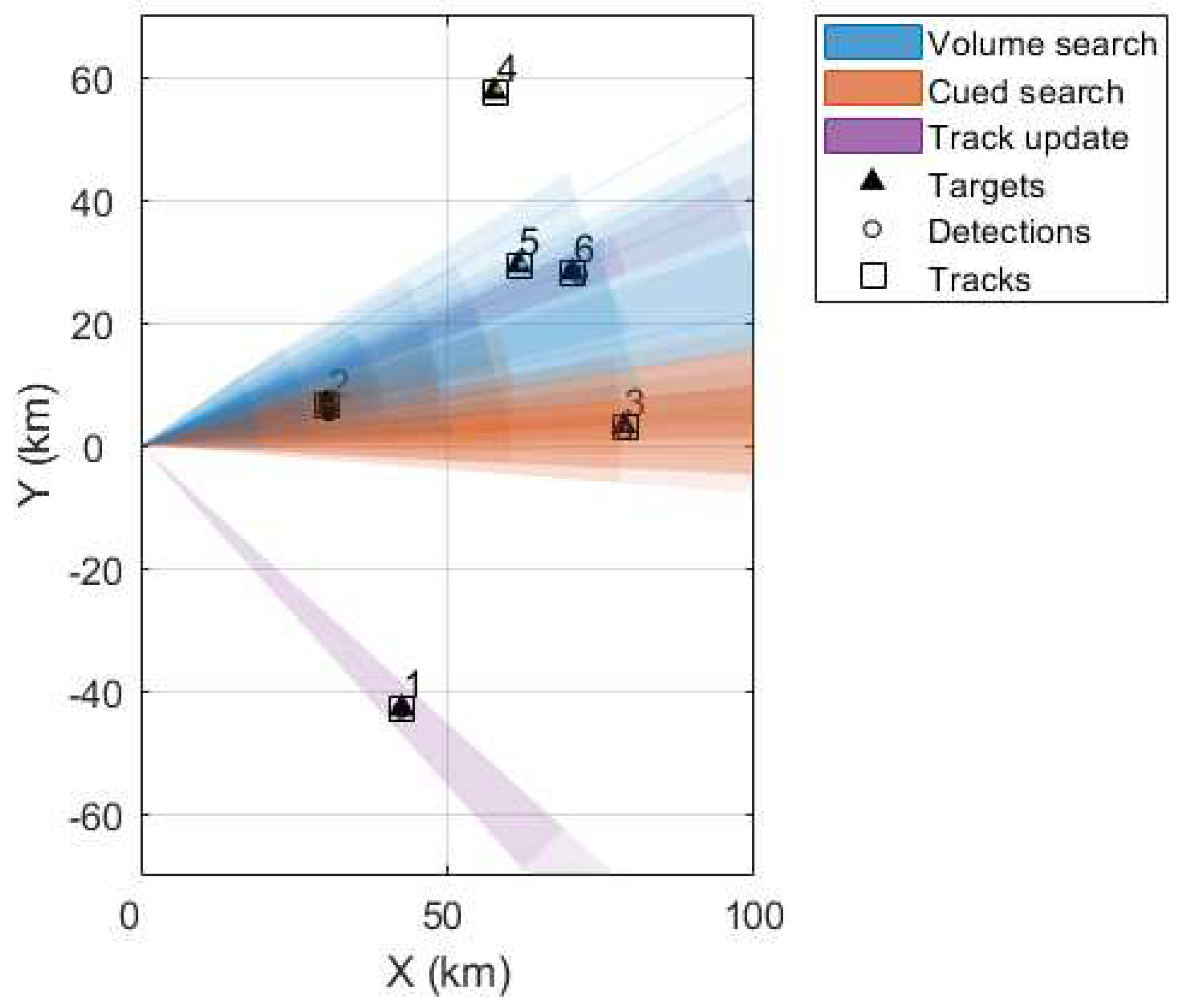
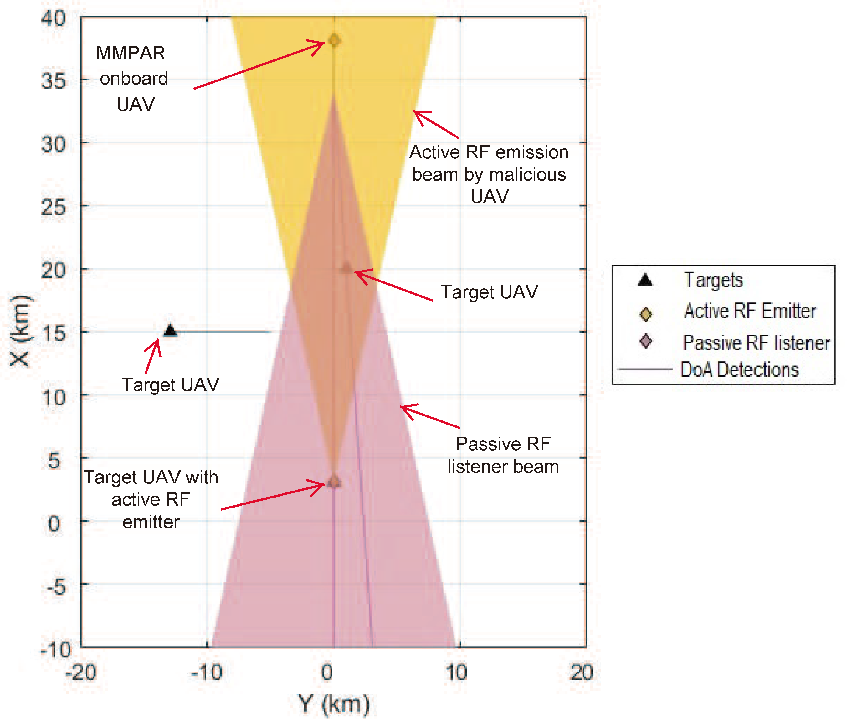
We are considering two UAV platforms, each equipped with an MMPAR. These UAVs are labeled as UAV1 and UAV2, respectively. They follow a straight-line trajectory at a constant velocity towards the targets. UAV1 has six targets in front of it, while UAV2 scans three targets. All targets are airborne and within the range of the radars. Figure 6 shows a snapshot of UAV1 carrying MMPAR scanning the six targets using volume, cued, and track beams. In Figure 7, an airborne platform carrying a malicious RF emitter emits a beam towards UAV2 carrying MMPAR.
The targets have assigned trajectories determined by their initial and final waypoints. The targets move with an average displacement of 26.6 km, 31.7 km, and 1.3 km in the x, y, and z coordinates, respectively, and their average velocity is 450 m/s. The RCS values of the targets are 1 m2 and 3 m2, and the Swerling1 RCS fluctuation model is employed for the simulations. The active RF emitter carried by one of the targets in Figure 7 has an EIRP of 200 dBi.
Figure 6. Volume search, cued search, and track beams are utilized by MMPAR onboard UAV1 to detect and track targets, with the six targets following distinct trajectories in the scenario.
Preprints 76460 g006
Figure 7. Onboard a malicious UAV, there is an active RF emitter. Meanwhile, the MMPAR onboard UAV2 generates a passive RF listener beam that can detect active RF emissions and determine their direction of arrival. This includes both direct (from active RF emitter) and reflected emissions from a target within the range of the active RF beam. The directions of arrival (DoA) are represented by straight lines.
Preprints 76460 g007
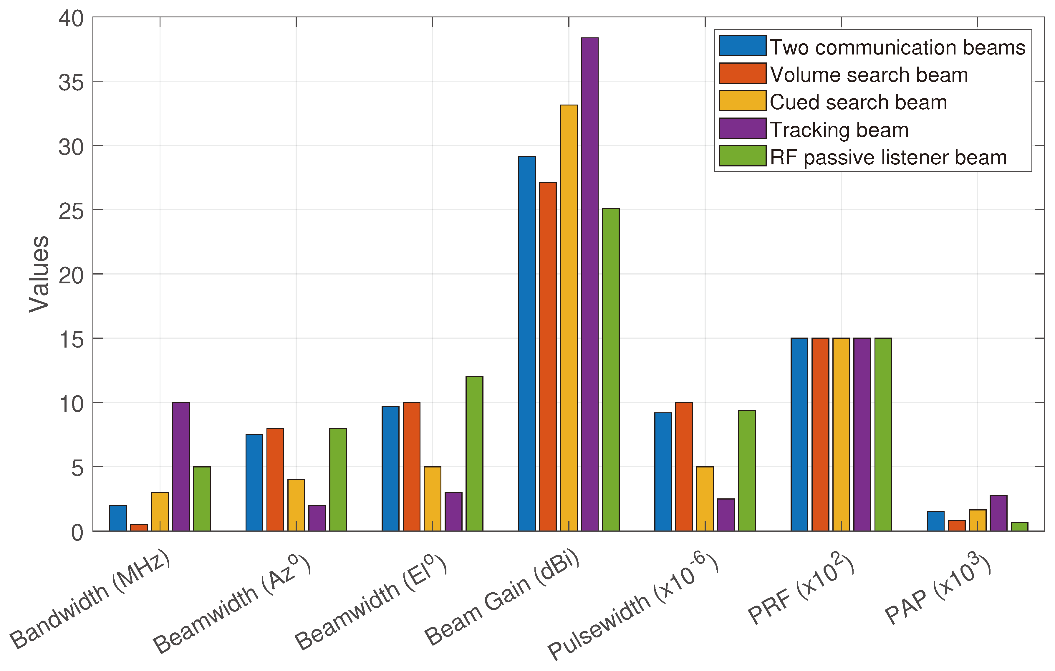
Figure 8. Resource distribution among the beams. The PAP presented here is for a peak transmit power of 150 × 10 3 .
Preprints 76460 g008

4.2. Results and Analysis

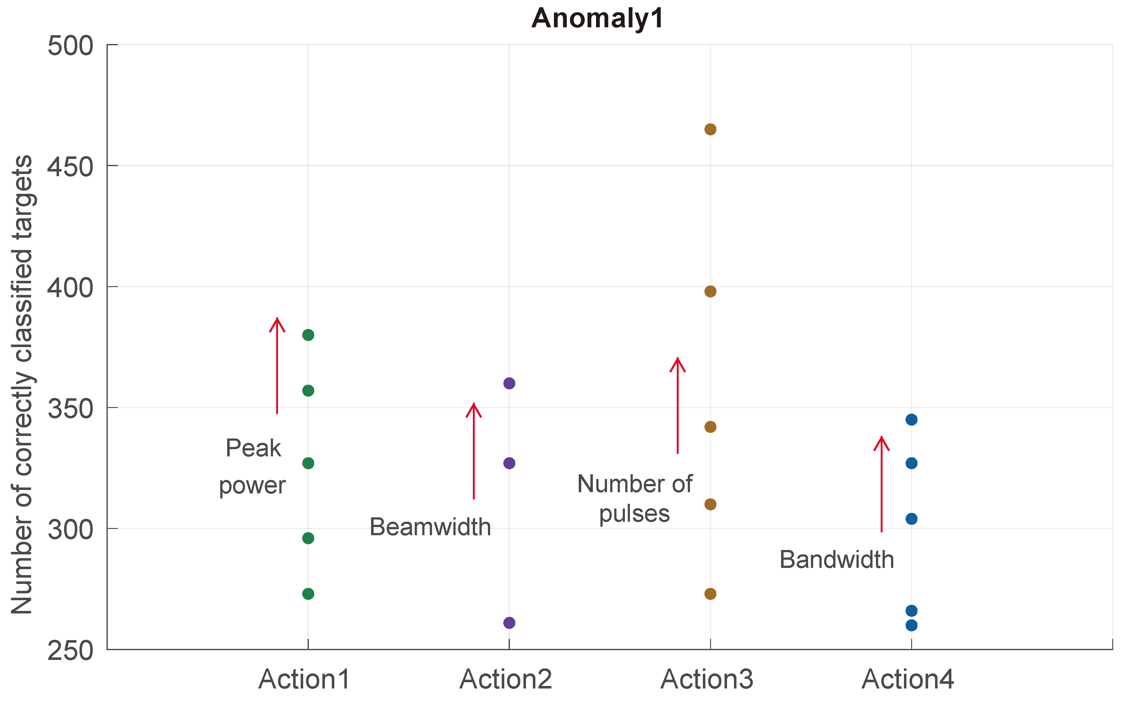
The simulations introduce anomalies to the radar environment by adding randomness according to (9). The simulation duration is 200 s, comprising 4000 update intervals. The first two anomalies and their respective priority actions for the MMPAR onboard UAV1 are shown in Figure 9 and Figure 10. For the first anomaly in Figure 9, the goal is to have above 300 correctly detected targets throughout the simulation duration, and if the number of correctly detected targets is 300 or less, it is considered an anomaly. The priority actions taken to remove the anomaly include increasing the peak power, reducing the beamwidth, increasing the number of pulses, and bandwidth. The peak power varies between 150 × 10 3 and 400 × 10 3 , the beamwidth is reduced by 1 degree in both the azimuth and elevation planes, the number of pulses is increased from 10 to 35, and the bandwidth increases from 10 × 10 6 to 35 × 10 6 . The results show that the priority actions help to increase the number of correctly detected targets above the anomaly threshold of 300.
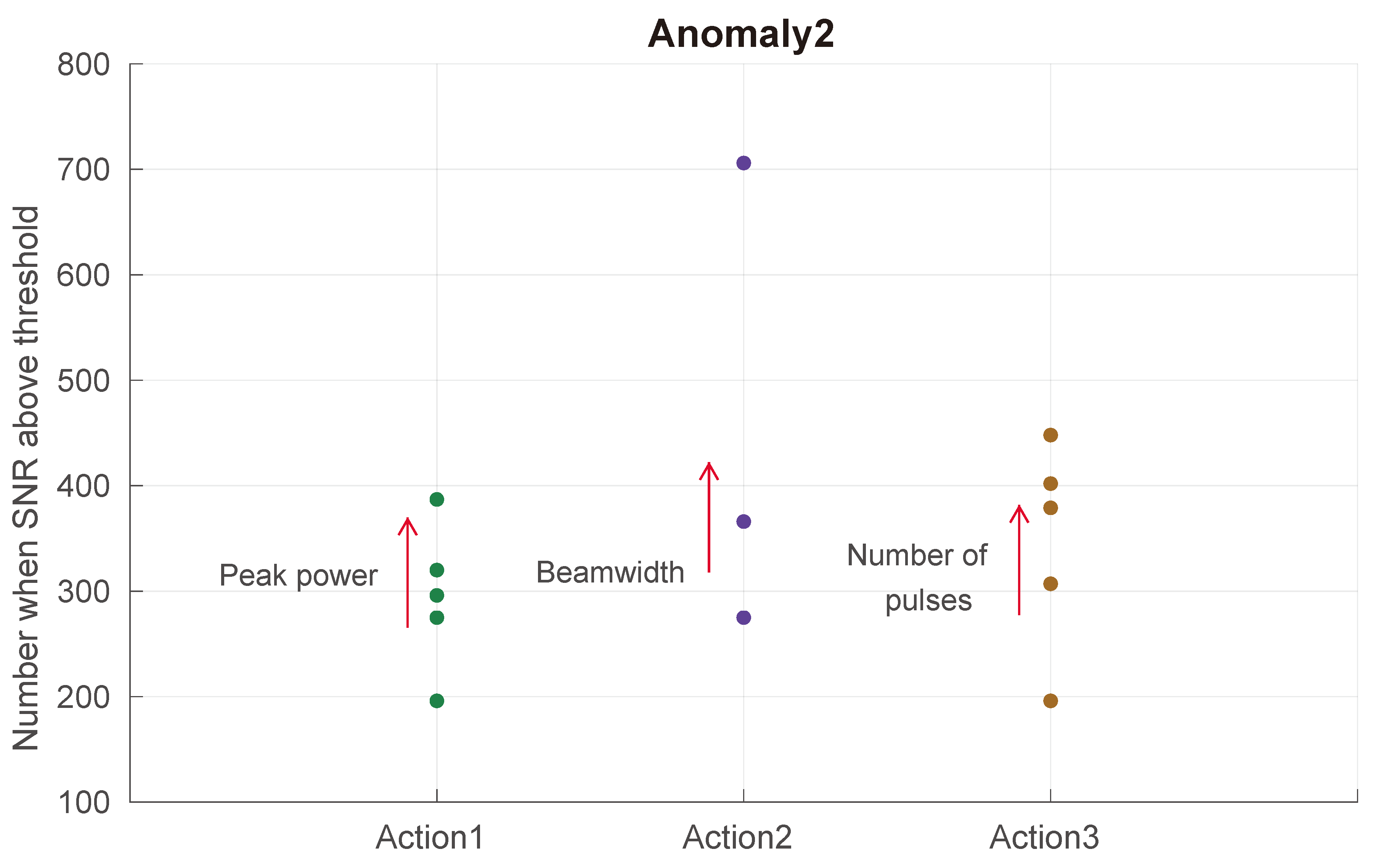
In Figure 10, the second anomaly from Table 6 is shown, and we aim to keep the number of targets detected above the SNR threshold of 10 dB above 300. The three priority actions selected based on the highest Q-values include increasing peak power, decreasing the beamwidth, and increasing the number of pulses. As illustrated in Figure 10, applying the priority actions increases the number of occurrences when the SNR of the detected targets is above the threshold. The other anomalies and corresponding actions from Table 6 can also be plotted.
Figure 9. Anomaly1 at MMPAR onboard UAV1 occurs when the number of correctly detected targets over a fixed simulation duration is less than 300. Corresponding actions are taken to remove the anomaly, which include varying the peak power in the range of 150 × 10 3 W: 50 × 10 3 : 400 × 10 3 W, the beamwidth [ 2 3 ] is reduced by 1 ° as [ [ 2 2 ] [ 1 2 ] [ 1 1 ] ], the number of pulses is changed as 10 : 5 : 35 , and the range of bandwidth change is as follows: 10 × 10 6 Hz: 5 × 10 6 : 35 × 10 6 Hz. These actions help increase the number of correctly detected targets.
Preprints 76460 g009
Figure 10. Anomaly2 occurs when the number of targets detected with an SNR above the 10 dB threshold is less than 300. Similar actions to those in Figure 9 are taken to remove the anomaly and increase the number of targets detected with an SNR above 10 dB.
Preprints 76460 g010
The MMPAR onboard UAV2 uses a passive RF listener beam to detect active RF emissions from a target UAV, as depicted in Figure 7. The frequency sweep is performed using the passive listener beam to detect the active emissions, and the direction of arrival is determined by the same beam, shown as a line in the figure. Another line in Figure 7 shows the detection caused by the reflection of RF energy from a non-emitting target within the emitter beam footprint towards the RF listener beam.

4.3. Comparison of RL with other AI Algorithms
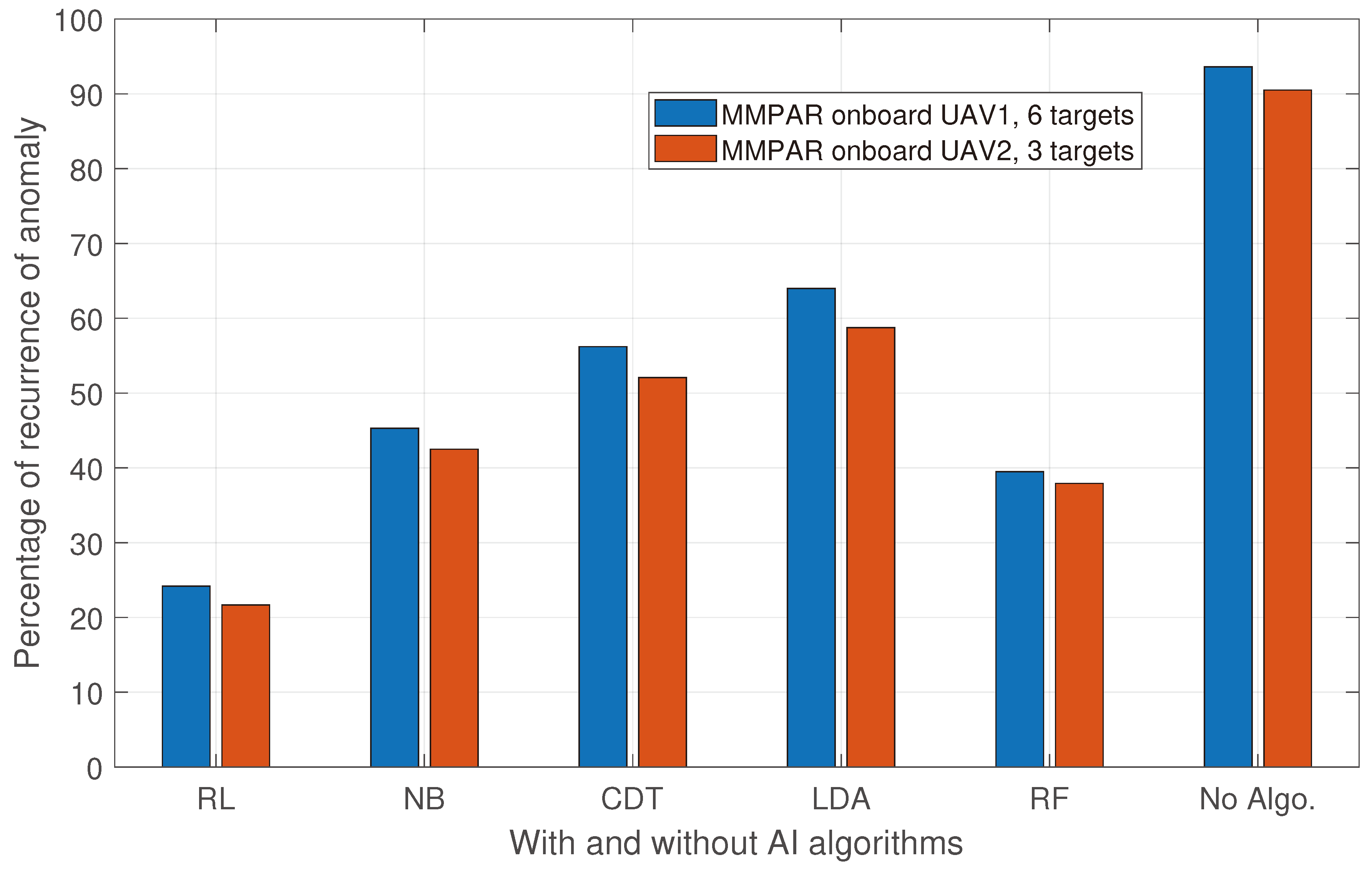
In addition to RL, we also utilize the four supervised AI algorithms discussed in Section 3.4 to address anomalies. These algorithms predict the best action to remove the anomaly, and we compare their effectiveness with the Q-learning RL algorithm. Specifically, we compare the percentage of anomaly recurrence after applying the optimal action, as outlined in Algorithm 3). Figure 11 shows the results of this comparison.
Figure 11 shows that RL outperforms other supervised AI algorithms in handling anomalies. This is mainly due to RL’s continuous situational awareness from environment feedback in the form of rewards and the ability to update its policy during runtime. In contrast, once a supervised AI algorithm is trained, it tries to find the best match based on training without taking any runtime feedback from the environment. Furthermore, the performance of supervised AI algorithms is expected to decrease in complex and dynamic scenarios with rapidly changing environments. Additionally, the recurrence percentage of anomalies is higher for all AI algorithms when six targets are present compared to three targets.
Figure 11. The percentage of anomaly recurrence after taking optimum actions based on Q-values is presented in the graph. The simulations were conducted over a duration of 200 seconds. It is observed that the highest percentage of anomaly recurrence occurs when no AI algorithm is used, while the lowest percentage is obtained using RL. Additionally, the percentage of anomaly recurrence is higher for six targets as compared to three targets.
Preprints 76460 g011

5. Conclusions and Future Work

In this work, we have used MMPAR onboard UAVs to detect, track, and classify malicious UAVs in a swarm. In addition to radar operation, the MMPAR onboard UAVs in our study can also support communications. During radar operation, we identify and remove anomalies in the detection, tracking, and classification using optimal actions. Multi-agent RL is utilized to select optimal actions for a given anomaly. The optimal actions are chosen based on the highest Q-values from Q-learning. We have also provided a performance comparison of RL with selected supervised AI algorithms. The results show that the RL-based approach is better at handling anomalies in a dynamic environment compared to supervised AI algorithms. In our future work, we plan to implement centralized multi-agent Q-learning and compare the results with the current decentralized multi-agent Q-learning.

References

  1. Khawaja, W.; Guvenc, I.; Matolak, D.W.; Fiebig, U.C.; Schneckenburger, N. A Survey of Air-to-Ground Propagation Channel Modeling for Unmanned Aerial Vehicles. IEEE Commun. Surv. & Tut. 2019, 21, 2361–2391. [Google Scholar] [CrossRef]
  2. Hall, O.; Wahab, I. The use of drones in the spatial social sciences. Drones 2021, 5, 112. [Google Scholar] [CrossRef]
  3. Beloev, I.H. A review on current and emerging application possibilities for unmanned aerial vehicles. Acta technologica agriculturae 2016, 19, 70–76. [Google Scholar] [CrossRef]
  4. Alghamdi, Y.; Munir, A.; La, H.M. Architecture, Classification, and Applications of Contemporary Unmanned Aerial Vehicles. IEEE Consum. Electron. Mag. 2021, 10, 9–20. [Google Scholar] [CrossRef]
  5. Custers, B. Future of Drone use; Springer, 2016. [Google Scholar]
  6. Khawaja, W.; Semkin, V.; Ratyal, N.I.; Yaqoob, Q.; Gul, J.; Guvenc, I. Threats from and countermeasures for unmanned aerial and underwater vehicles. Sensors 2022, 22, 3896. [Google Scholar] [CrossRef] [PubMed]
  7. Guvenc, I.; Koohifar, F.; Singh, S.; Sichitiu, M.L.; Matolak, D. Detection, Tracking, and Interdiction for Amateur Drones. IEEE Commun. Mag. 2018, 56, 75–81. [Google Scholar] [CrossRef]
  8. Svanström, F.; Alonso-Fernandez, F.; Englund, C. Drone Detection and Tracking in Real-Time by Fusion of Different Sensing Modalities. Drones 2022, 6, 317. [Google Scholar] [CrossRef]
  9. Ezuma, M.; Ozdemir, O.; Anjinappa, C.K.; Gulzar, W.A.; Guvenc, I. Micro-UAV Detection with a Low-Grazing Angle Millimeter Wave Radar. In Proceedings of the Proc. IEEE Radio and Wireless Symp. (RWS); 2019; pp. 1–4. [Google Scholar] [CrossRef]
  10. Gong, J.; Yan, J.; Li, D.; Kong, D. Detection of Micro-Doppler Signals of Drones Using Radar Systems with Different Radar Dwell Times. Drones 2022, 6, 262. [Google Scholar] [CrossRef]
  11. Jian, M.; Lu, Z.; Chen, V.C. Drone detection and tracking based on phase-interferometric Doppler radar. In Proceedings of the Proc. IEEE Radar Conf. 2018; pp. 1146–1149. [Google Scholar] [CrossRef]
  12. Hoffmann, F.; Ritchie, M.; Fioranelli, F.; Charlish, A.; Griffiths, H. Micro-Doppler based detection and tracking of UAVs with multistatic radar. In Proceedings of the Proc. IEEE Radar Conf. 2016; pp. 1–6. [Google Scholar] [CrossRef]
  13. Aldowesh, A.; Shoaib, M.; Jamil, K.; Alhumaidi, S.; Alam, M. A passive bistatic radar experiment for very low radar cross-section target detection. In Proceedings of the Proc. IEEE Radar Conf. 2015; pp. 406–410. [Google Scholar] [CrossRef]
  14. Yao, Y.; Zhao, J.; Wu, L. Waveform optimization for target estimation by cognitive radar with multiple antennas. Sensors 2018, 18, 1743. [Google Scholar] [CrossRef] [PubMed]
  15. Haykin, S. Cognitive radar: a way of the future. IEEE Signal Process. Mag. 2006, 23, 30–40. [Google Scholar] [CrossRef]
  16. Metcalf, J.; Blunt, S.D.; Himed, B. A machine learning approach to cognitive radar detection. In Proceedings of the Proc. IEEE Radar Conf. 2015; pp. 1405–1411. [Google Scholar] [CrossRef]
  17. Smith, G.E.; Gurbuz, S.Z.; Brüggenwirth, S.; John-Baptiste, P. Neural Networks & Machine Learning in Cognitive Radar. In Proceedings of the Proc. IEEE Radar Conf. 2020; pp. 1–6. [Google Scholar] [CrossRef]
  18. Thornton, C.E.; Kozy, M.A.; Buehrer, R.M.; Martone, A.F.; Sherbondy, K.D. Deep Reinforcement Learning Control for Radar Detection and Tracking in Congested Spectral Environments. IEEE Trans. on Cognitive Commun. and Netw. 2020, 6, 1335–1349. [Google Scholar] [CrossRef]
  19. Ahmed, A.M.; Ahmad, A.A.; Fortunati, S.; Sezgin, A.; Greco, M.S.; Gini, F. A Reinforcement Learning Based Approach for Multitarget Detection in Massive MIMO Radar. IEEE Trans. on Aerosp. and Electron. Syst. 2021, 57, 2622–2636. [Google Scholar] [CrossRef]
  20. Yang, T.; De Maio, A.; Zheng, J.; Su, T.; Carotenuto, V.; Aubry, A. An Adaptive Radar Signal Processor for UAVs Detection With Super-Resolution Capabilities. IEEE Sensors J. 2021, 21, 20778–20787. [Google Scholar] [CrossRef]
  21. Wu, Q.; Wang, H.; Li, X.; Zhang, B.; Peng, J. Reinforcement learning-based anti-jamming in networked UAV radar systems. Appl. Sci. 2019, 9, 5173. [Google Scholar] [CrossRef]
  22. Chen, Y.J.; Chang, D.K.; Zhang, C. Autonomous Tracking Using a Swarm of UAVs: A Constrained Multi-Agent Reinforcement Learning Approach. IEEE Trans. on Veh. Technol. 2020, 69, 13702–13717. [Google Scholar] [CrossRef]
  23. Mendis, G.J.; Wei, J.; Madanayake, A. Deep learning cognitive radar for micro UAS detection and classification. In Proceedings of the Proc. IEEE Cogn. Commun. for Aerosp. Appl. Workshop (CCAA); 2017; pp. 1–5. [Google Scholar] [CrossRef]
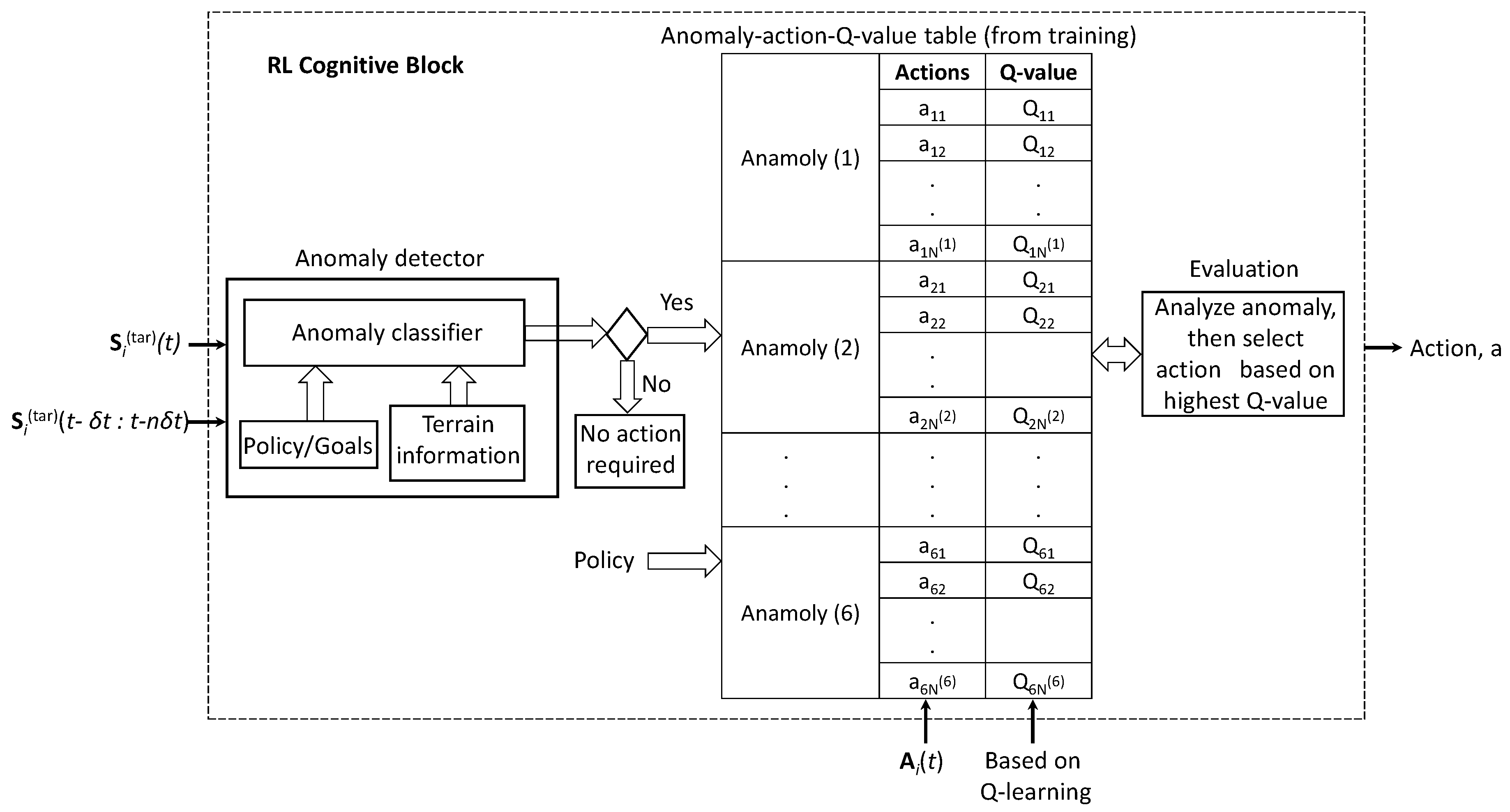
Figure 4. The RL cognitive block for the i th MMPAR onboard a UAV at time instance t takes in the states of the target, S i ( tar ) ( t ) , and S i ( tar ) ( t δ t : t n δ t ) . Additionally, the radar parameters and position of the radar platform are provided as an action set, A i ( t ) . The Q-values in the table are obtained based on rewards for state-action pairs (see Algorithm 2). The RL follows a simple policy of removing anomalies through optimum actions, selecting the best action based on Q-value. During the evaluation phase, the Q-values can be updated (see Algorithm 3).
Preprints 76460 g004
Table 1. Comparison of our approach with other popular radar-based approaches in the literature.
Functionalities Our approach [19] [20] [21] [22] [23]
Phased array multifunction,
multibeamsteering
(simultaneously) and
adaptive beam scheduling
Airborne and mobility in air
Networked radar nodes
Multi-agent RL
Anomalies in the detection,
tracking, and classification
identification and removal
Cognitive or adaptive
adjustment of radar parameters
or radar platform
position adjustment
Multi-target detection/
tracking/classification
Performance degradation in
complex and dynamic
environments
No No Not reported Not reported No Not reported
Communications relaying
capability
in addition to radar operation
Table 3. List of anomalies observed at n δ t update intervals.
Serial # Anomalies
1 Targets not correctly detected (because targets are not resolved in range and angular domains).
2 Targets detected with SNR below a threshold (either due to clutter or RF interference).
3 Velocity variations above a threshold.
4 RCS fluctuations above a threshold.
5 Active RF emissions from malicious UAVs.
6 Classification of targets change (due to the above listed anomalies).
Table 7. Simulation parameters of the radar.
Serial # Radar parameters Parameter values
1 P ( TX , max ) : P ( TX , min ) 100 × 10 3  W :  500 × 10 3  W
2 f ( c , max ) : f ( c , min ) 1.2  GHz :  4.3  GHz
3 B W ( max ) : B W ( min ) 10 × 10 6  Hz :  50 × 10 6  Hz
4 θ ( b , max ) : θ ( b , min ) , ϕ ( b , max ) : ϕ ( b , min ) [ 15 ° : 1 ° ] [ 14 ° : 1 ° ]
5 P R F ( max ) : P R F ( min ) 1400 : 1600
6 Number of pulses 5 : 25
7 W a v Noise radar waveform
8 P o l Vertical
9 Radar noise figure 5 dB
Disclaimer/Publisher’s Note: The statements, opinions and data contained in all publications are solely those of the individual author(s) and contributor(s) and not of MDPI and/or the editor(s). MDPI and/or the editor(s) disclaim responsibility for any injury to people or property resulting from any ideas, methods, instructions or products referred to in the content.
Copyright: This open access article is published under a Creative Commons CC BY 4.0 license, which permit the free download, distribution, and reuse, provided that the author and preprint are cited in any reuse.
Prerpints.org logo

Preprints.org is a free preprint server supported by MDPI in Basel, Switzerland.

Subscribe

© 2024 MDPI (Basel, Switzerland) unless otherwise stated