1. Introduction
The COVID-19 pandemic caused a significant disruption in the standard of living around the world, leaving behind an entirely new behavior in commercial patterns and business ideas that hardly affected electrical consumption (Alasali et al., 2021, Baker et al.,2020). In 2020, to decrease the number of people infected, governments in many countries established lockdowns and strict restrictions on their inhabitants, closing educational centers, and leisure businesses which limited people from leaving their places just in emergencies (Baker et al.,2020, Siksnelyte-Butkiene et al., 2021). Only the essential workers in the health systems or other crucial sectors were allowed to commute. These decisions highly impacted human lifestyle, along with the contraction in industrial activities, which eventually led to a significant reduction in greenhouse gas emissions and energy demand (Smith et al., 2021, Abu-Rayash et al., 2020). In the U.S., states such as Florida and California reported changes in the seasonal energy consumption pattern during the lockdowns. For instance, the latter outlined a reduction of up to 12 %; while for Florida, the changes did not imply a reduction in all cases (Navon et al., 2021).
In Europe, studies showed that COVID-19 impacted the level of weekly electricity demand, and even after it, consumption patterns have permanently been modified (Werth et al., 2020). Latin America and the Caribbean experimented with similar conditions, and most countries displayed a decrease to a greater or lesser extent during 2020 compared to non-COVID scenarios; Bolivia and Peru showed shifts of about 30 % (Sanchez-Údeba et al., 2022). Unsurprisingly, small businesses dropped 22 % in the first months of 2020, with over 3.3 million stores inactive just in the U.S. The reason mentioned before and the acceleration to a digital age that many businesses put on have left the energy industry in a high uncertainty situation (Soyars et al., 2021). The oil and Gas sector was one of the mostly impacted by COVID-19; as the economic activity started to decelerate across the globe, claims for fossil fuel and derivatives dove (Camp et al., 2020). As a result, analysis of oil and gas prices and consumption became critical for investors, companies, and governments since they were looking for solutions to the imminent energy crisis. In this article, an investigation was carried out to analyze the changes in petroleum fuel consumption patterns for power generation and the price of petroleum fuel simultaneously caused by the COVID-19 pandemic.
An accurate forecast is an essential and effective solution for energy management systems allowing them to keep a reliable source of power for the industry and houses even during disruptive events such as the COVID-19 pandemic or new outbreaks like monkeypox. Forecasting models are key in the power system operation and energy demand (Alasali et al., 2018). However, predicting the accuracy of those models is challenging because it depends on factors like unpredictable and fluctuating behavior, rather than clear patterns in the data. Human activity also plays a complex role, making accurate predictions difficult. Since COVID-19 appeared, many studies have been published analyzing the effect of the pandemic on renewable energy sources, fossil fuels, energy consumption, and human behavior (Agdas et al., 2020). Nevertheless, most of them have ignored several factors that also impacted the energy demand and oil prices, causing biased results.
The oil and Gas sector is one of the most influential industries globally, directly impacting society patterns of consumption and, thus, behavior. Oil price influences the costs of other production and manufacturing. Having a clear idea of how the oil and gas prices demeanor is vital for governments, companies, and investors. However, it is biased under many other factors, such as political insatiability in petroleum producer countries, economic recessions, and energy demand. During COVID, as the economy slowed, oil prices reached a historical minus zero caused by the drop in demand and an unexpected increase in supply, which led to the collapse (OECD 2020). Subsequently impacting prices for refined petroleum products and other downstream items, notably gasoline. As economies reopened, the initial price downturn gave way to reduced oil production and some renewed demand. As a result, prices for oil products partially recovered (Camp et al., 2020).
In the present study, data was taken from the "U.S. Energy Information Administration" over seven years, from 2016 to 2022, to analyze and investigate the oil fuel consumption for power generation and fossil fuel prices during the pre, during, and post-pandemic periods. The data covered the entire United States. The whole country was taken into consideration to avoid the uncertainty and biases of fuel consumption and price. The increases in the annual population, weather, and seasonal factors were considered to investigate the impact of the COVID-19 pandemic. Therefore, the forecasting has been performed using all benchmark methods, STL, ETS, and ARIMA methods, to compare multiple methods and pick the best one that predicts the general pattern of change in price and consumption irrespective of seasonal and pandemic impact.
Later, to isolate only the pandemic impact, the ARIMAX model has been used by eliminating all seasonal effects. ARIMA models are employed to forecast time series data based solely on its own past values to capture the moving average (MA) and autoregressive (AR) components and take stationarity into account through differencing (Kotu et al., 2019, Ray et al., 2020). Without considering any external inputs, ARIMA models presume that the underlying data is created by combining its own historical values. In contrast, exogenous variables (X), which are outside elements that could affect the time series, are included in ARIMAX models to further extend ARIMA (Ray et al., 2020, Jain G. et al., 2017). Exogenous variables allow ARIMAX models to capture the influence of outside variables on the time series behavior in addition to the autocorrelation and moving average features of the data. ARIMAX models are particularly suitable for predicting irregular behavior because they can account for the influence of external factors that may contribute to the irregularity or unpredictability in the time series (Kim et al., 2023). These external factors could include seasonality, weather conditions, economic indicators, or other relevant variables that may affect the time series behavior. By incorporating these exogenous variables, ARIMAX models can better capture and explain irregular patterns, leading to more accurate predictions (Kim et al., 2023). Therefore, several exogeneous variables like temperature, price and mileage traveled have been incorporated upon which petroleum fuel consumption is likely to depend. The ARIMAX model is supposed to capture the stochastic and non-smoothing behavior of the pandemic on petroleum fuel consumption and price in this article.
There has been plenty of research done to understand the impact of COVID-19 on different sectors, including fluctuation of energy demand (Kang et al., 2021). But none of the work so far has investigated the impact of only pandemic itself in future forecasting of fuel consumption. Also, the volatility of fuel price has been studied due to COVID-19 in previous literature. But there is hardly any explicit and significant research performed on how fuel prices will be affected only due to pandemic by isolating the COVID impact. Also, the correlation of other exogeneous variables apart from seasonal influence; like mileage travelled, average temperature, etc., was not studied in the early literature to provide an accurate forecast of fuel price and consumption for any future pandemic period. The added value and the essential novelty of this paper revolve around the interconnectedness of the demand analysis and forecasting of consumption and cost during the COVID-19 pandemic, considering the new demand and behavioral and cultural changes. It will also examine the impact of the COVID-19 pandemic as an exogenous variable on the forecast model performance, which will help to predict the anomalies if any identical kind of pandemic appears in the near future. Moreover, it will assist to differentiate the regular forecasting of fuel price and consumption from the pandemic impact which can be utilized by designated authority for energy plan and distribution depending on different scenarios.
2. Fuel Consumption Pattern Analysis
In the United States and generally around the globe, governments implemented travel restrictions and an economic slowdown to mitigate the coronavirus outbreak causing the drop in petroleum products consumption to its lowest level in more than 30 years. In the first quarter of 2020, the total petroleum U.S. demand averaged 14.1 million (b/d), which was 31% lower than in the same period in 2019 (Camp et al., 2020). This changed the whole product supply chain, mainly in motor gasoline, distillate fuel oil, jet fuel, and chemical feedstocks.
Based on a machine-learning model, Ou et al. (2020) included pandemic scenarios and trip activities to forecast future U.S. fuel demand showing a decrease of 22% in gasoline consumption in comparison with non-COVID schemes. Güngör et al. (2020) analyzed the effect of COVID-19 on Turkish gas consumption from 2014 to 2020; their results displayed variations of up to 30% after and before the global event. Tian et al. (2021) studied the impact of COVID-19 on urban transportation in Canada, with a reduction of at least 60% in the main cities, which aligns with the reports of petroleum product consumption reduction; in the case of diesel up to 49.8 % drop in May 2020. Smith et al. (2020) showed results except for fossil fuel consumption to reach the pre-crisis level in 2023. The COVID-19 will continue impacting petroleum products demand and, thus, many aspects of human behavior. This study will analyze seasonality and autocorrelation to distinguish the seasonal and non-seasonal impact on fuel consumption. The forecasting model has been selected according to the nature of the data.
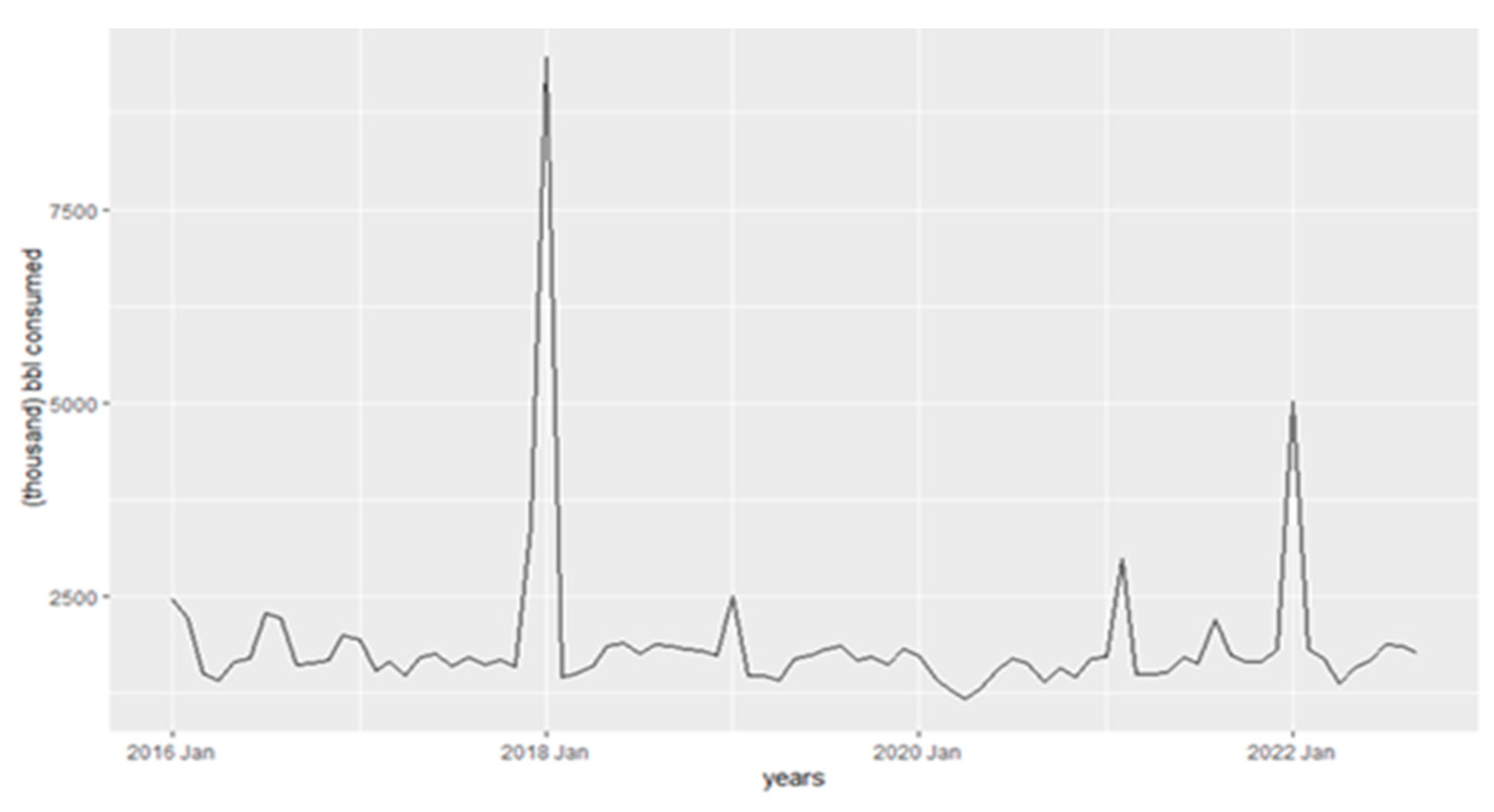
Figure 1 exhibits the seasonality of petroleum fuel consumption in the United States, showing the peak in oil barrels consumed at the beginning of the year, then it decreases and increases again during summer. Clearly, 2020 and 2018 are the outliers in this analysis.
2.1. Seasonality Analysis of Petroleum Fuel Consumption
The seasonality of U.S. petroleum fuel consumption for five years has been explored in this segment. Generally, during non-pandemic years gasoline and petroleum products consumption exhibit seasonal patterns, principally increasing in the summer season and dropping in the winter due to the more human activity and air conditioning usage to avoid the high temperatures. Other peaks in consumption are due to holidays such as Thanksgiving. The measures taken by many countries to reduce the impact of the Coronavirus, such as closing schools and industries, implementing remote work, and enforcing lockdowns, greatly affected the usual patterns of oil demand. This impact was particularly notable in petroleum products like gasoline and diesel. These dramatic changes in human lifestyle immensely influenced the environment and the oil supply chain. Most countries tried to reduce oil and gas consumption in favor of renewables, increasing the crisis in the sector.
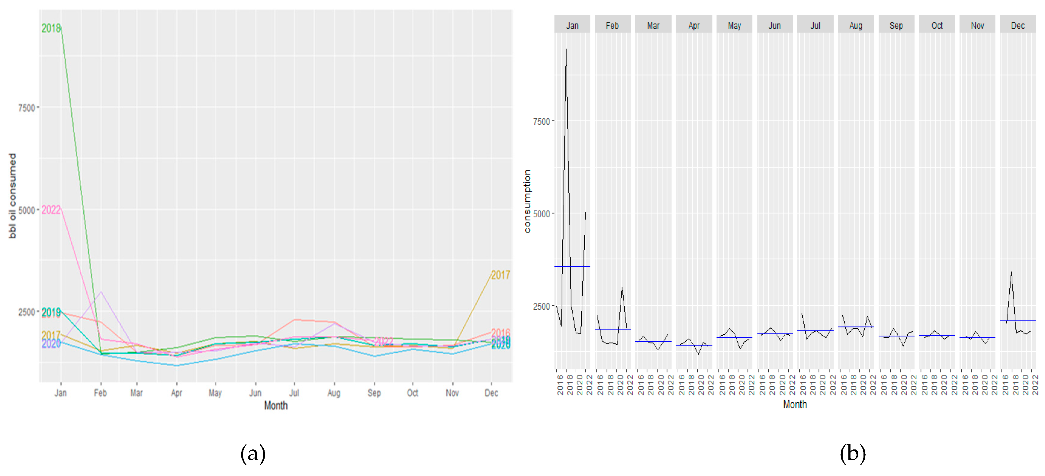
Figure 2a displays the monthly petroleum fuel consumption from 2016 to 2022 in the U.S. It shows how the energy demand in 2020 became the lowest in the dataset, with clear lows in April and September during the lockdowns.
From the seasonal analysis of monthly fuel consumption in
Figure 2b, it is clearly seen that the consumption was higher at the begging of every year (January). It then drastically dropped until the summertime, which went back to increase consumption. Once again, the impact of COVID is clear, with 2020 having the lowest peak every month; also, the monthly seasonality in this series times has been disrupted due to the reason previously mentioned.
2.2. Autocorrelation Analysis of Fuel Consumption
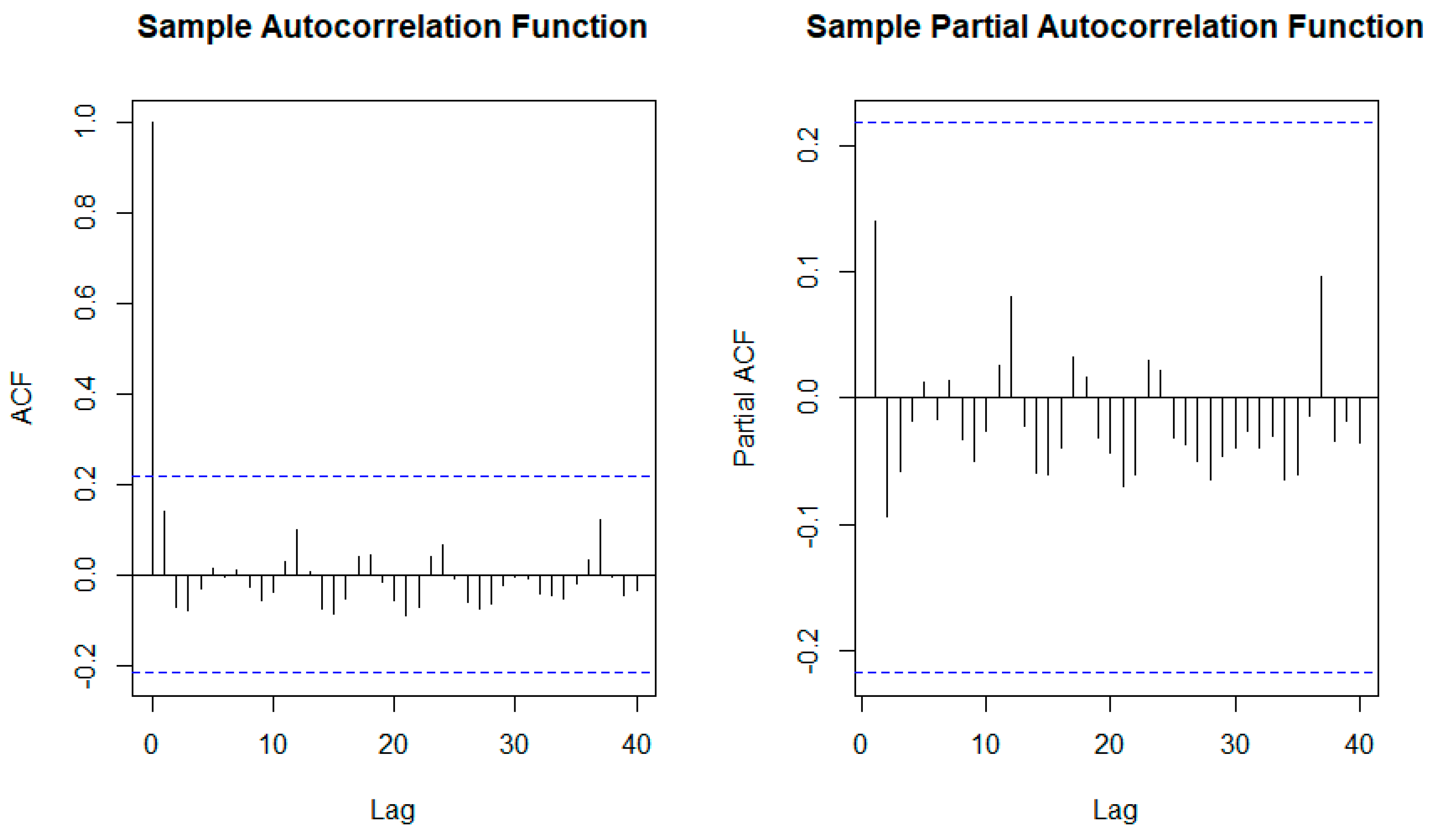
This section aims to find the time correlation in the fuel consumption time series and then remove it to show only the demand reduction related to the pandemic. To select any correlation between the fuel consumption in the time series, the partial autocorrelation function (PACF) was calculated, as shown in
Figure 3.
The PACF plot shows the correlation between the fuel consumption time series at lag t (L
t) for up to a specific number of lags. The PACF can be mathematically described as in Equation (1) (Sambran et al., 2008; Momani et al., 2016). The PACF analysis aims to find the relationship between the two time series points without considering the effect of all time points (lags) in between. In contrast, the autocorrelation function (ACF) is used to find the correlation between the consumption time series for different lags (seasonal or calendar patterns). However, the previous consumption analysis shows a lack of seasonality in 2020 during the COVID-19 pandemic compared to last year. Therefore, PACF is used in this section to find notable demand trends that are not seasonal. The PACF, as shown in
Figure 3b, presents the correlation between the electrical demand time series and the lagged points, at lag k, after removing all time series points (1, 2, ..., k - 1) between them (Amini et al., 2016 and Cui et al., 2015).
The PACF plot does not show any significant values occurring or repeating, indicating the lack of seasonality in fuel consumption for power generation. In
Figure 3, ACF and PACF are used to detect the seasonality of the dataset. However, the COVID pandemic in 2019 makes the data do not follow a seasonality. The significant spike at lag 1 in the ACF suggests a non-seasonal MA (1) component and PACF shows no pattern.
2.3. Peak Consumption Analysis
Table 1 displays the petroleum consumption statistical data such as maximum, minimum, and average amounts at monthly intervals. The results showed that there was a significant decrease in oil demand in 2020 as compared to previous years. For instance, the peak oil demand decreased from 2,506 million barrels (Mbl) in 2019 to 1,741 Mbl in 2020. The peak demand in 2020 was reduced by 49% and 81% compared to 2017 and 2018, respectively. Similarly, the minimum and mean oil demand in 2020 were lower than in previous years. In 2020, petroleum demand hit a record low of 1,169 Mbl, down from 1,451 Mbl in 2018 and 1,417 Mbl in 2019. In comparison to 2019 and 2018, 2020 exhibited a reduction of 17% and 19%, respectively. The outbreak of COVID-19 and subsequent lockdowns caused an immediate shift in peak oil and energy demands in the U.S. from March to May 2020, as a reduction in energy usage and transportation needs was observed. This study considers the data available on the US Energy Information Administration (EIA) website [9] up until August 2022. The maximum, minimum, and average are calculated over all the months. The fuel consumed in 2020 refers to the average fuel consumed over the year.
The following empirical equation has been used to calculate the change of fuel consumption with respect to pandemic year 2020:
It is clear that the fuel consumption started to increase after the onset of pandemic, particularly in 2022, with almost 68% increase for maximum consumption, 10% increase for minimum consumption and 28% increase for average consumption compared to pandemic year 2020. This occurred due to the opening of the industrial and business sectors after the pandemic lock-down was over.
3. Fuel Price Pattern Analysis
As global economy industries slowed down considerably, demand for oil and petroleum derivatives fell precipitously. In January 2020, oil prices plummeted after China decreased 20 % fossil fuel imports due to the increased number of COVID-19 cases in the country, directly impacting the oil price, which dropped to 14.3 %. Oil barrel prices are established internationally by the free market. Thus, the prices in the United States reflect the global scenario. On April 20, 2020, an oversupply of oil led to an unprecedented collapse in the raw material price, reaching -
$37 a barrel.
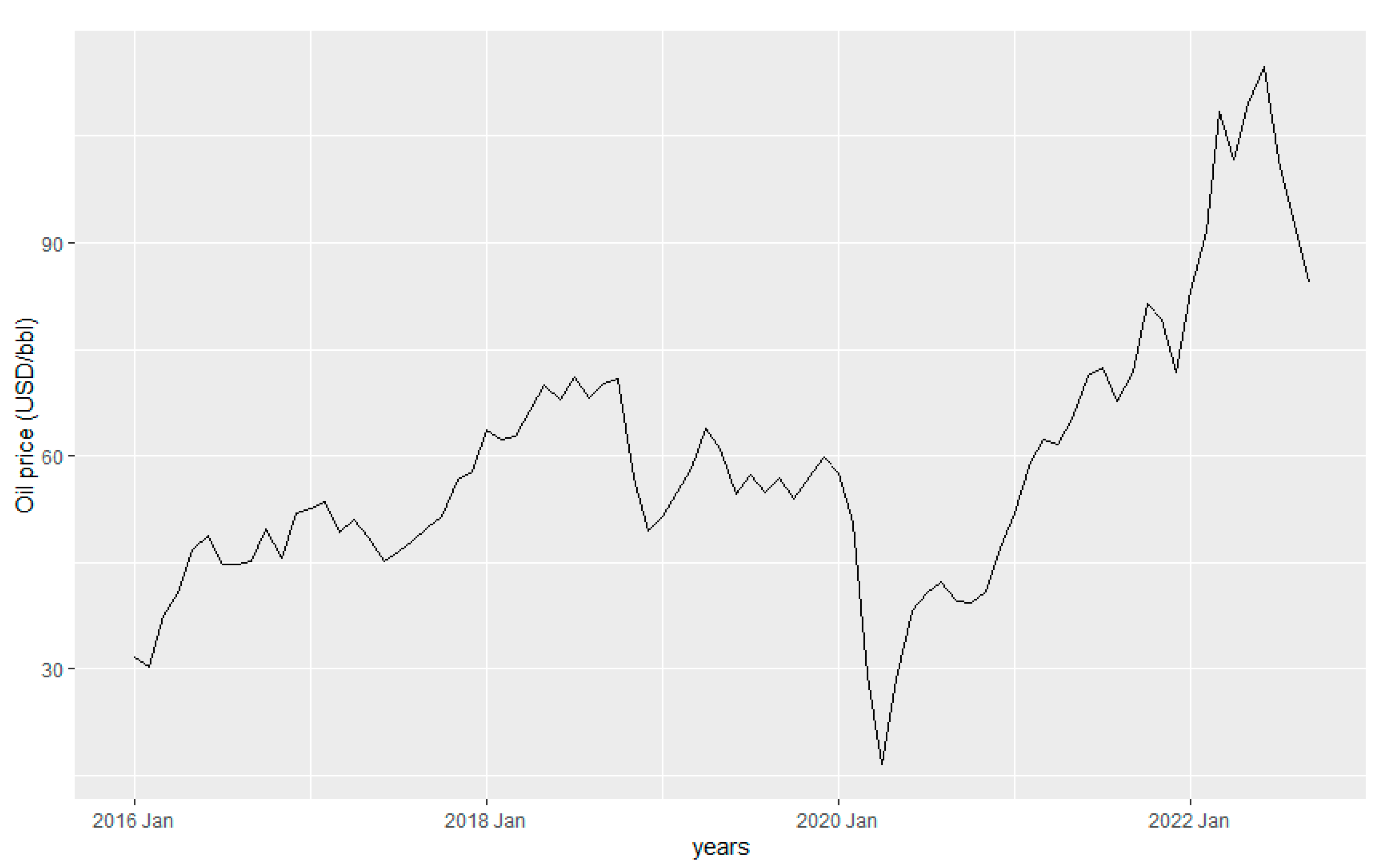
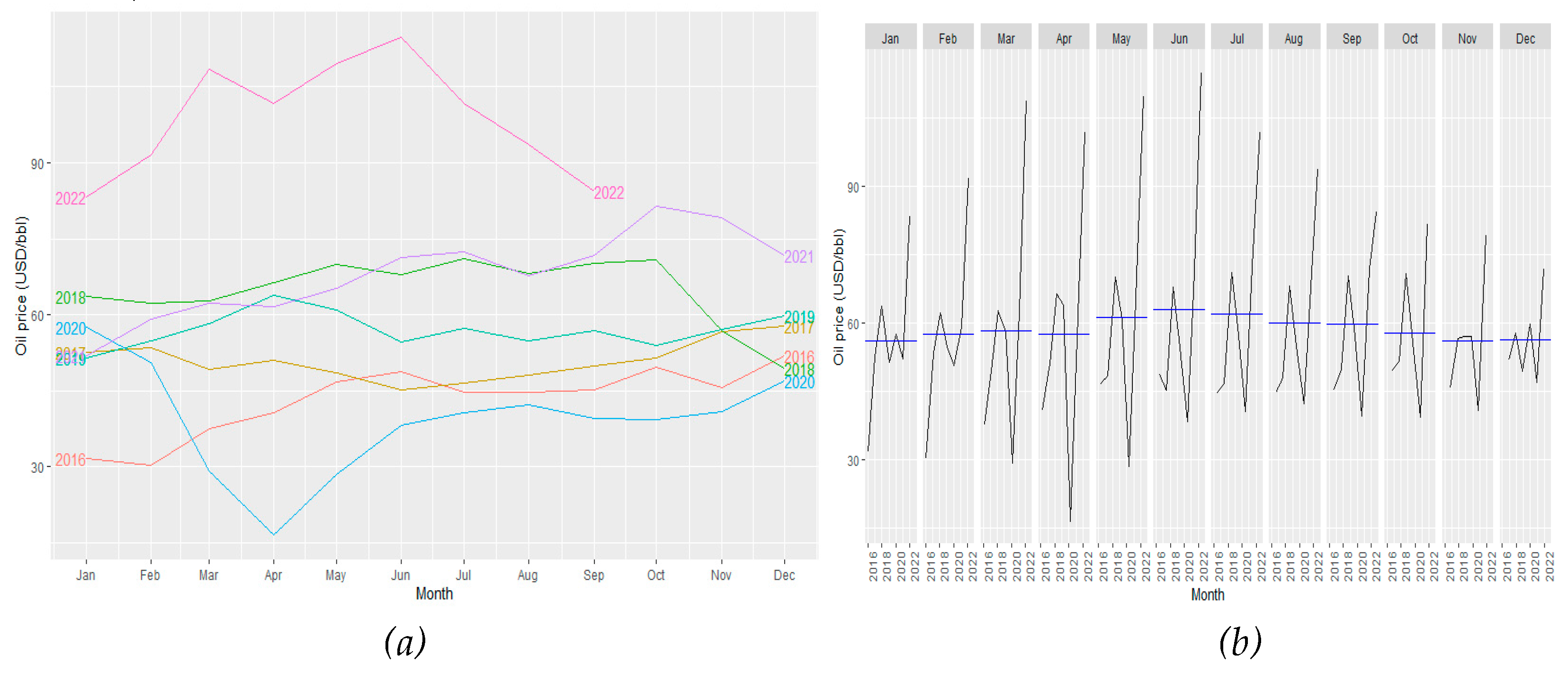
Figure 4 shows the oil price from 2016 to 2022, displaying the lowest price during 2020. It also shows the rapid upturn after the lockdowns and the recovery of the economy (Water et al., 2020)
3.1. Seasonality Analysis of Petroleum Fuel Price
Compared to petroleum consumption, fuel prices seem not to follow a seasonal pattern. This is mainly due to many factors that affect the oil and gas industry. For instance, the variation in demand and storage capacity in non-producer nations and the rising in the supply from oil-producer countries cause the price not to follow any seasonal or trend patterns. This statement has been observed in
Figure 5, where from 2016 to 2022, there was not a single year that followed such tendencies (Camp et al., 2020).
3.2. Autocorrelation Analysis of Fuel Price
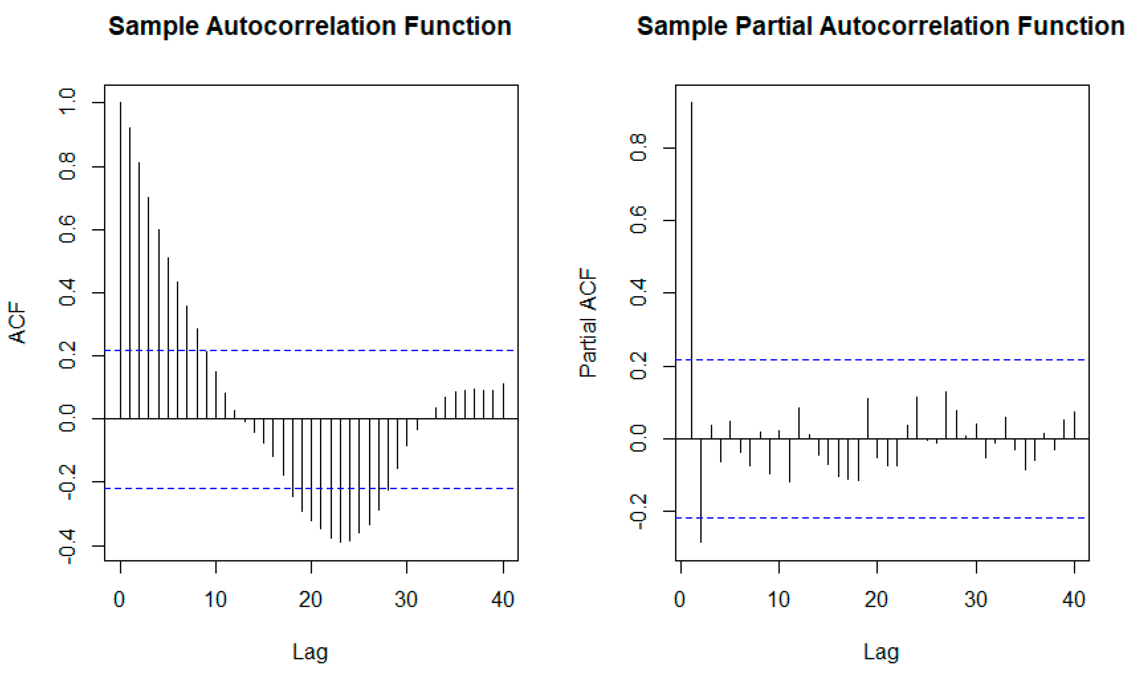
Figure 6 displays the ACF and PACF for the oil price (2016-2022). ACF shows a pattern associated with cycling data, which is complex and needs moving average MA (28) to be solved. In the case of the PACF, it shows that an autoregressive of the order two AR (2) model is needed. Since AR (2) is more straightforward, it is used to face this problem.
3.3. Peak Price Analysis
Table 2 exhibits the statistics for the oil price dataset, such as maximum, minimum, and mean values at monthly intervals. The results reveal that maximum, minimum, and average prices in 2020 were substantially lower than in prior years, especially from 2017, since the costs were recovered from the previous petroleum prices crisis. For example, in 2018 peak price was
$70.98, which is 18 % higher than in 2020. Furthermore, the minimum price in 2020 is considerably less than any other year, with at least a difference of 46 % (between 2016 at
$30.92 and 2020 at 16.55), with oil prices reaching the historical minimum for the 2010s. The following empirical equation has been used to calculate the percent reduction of fuel price with respect to pandemic year 2020:
It is clearly evident that the fuel price started to recover after the pandemic and increased almost 50% for maximum price, 80% for minimum price and 59% increased for average price at 2022 compared to pandemic year 2020. This happened due to the opening of all industrial and business sectors after pandemic lock-down was over.
4. Forecasting Model for Fuel Consumption
Forecasting models are generally developed to predict demand profiles and follow fluctuating demand (Santra et al., 2019). As illustrated before, the stochastic and non-smooth behavior of petroleum fuel consumption during and after the COVID-19 pandemic increases the challenges of accurately predicting the demand compared to previous years. Typically, points are used to forecast with a single estimate value for each time step (Park et al., 2020). However, this is mainly limited to the time-series data and cannot capture the degree of uncertainty in the data that much. In highly stochastic and unpredicted conditions, a forecast model with the ability to handle new and unpredicted conditions (such as the COVID-19 pandemic) and work under different degrees of uncertainty is required. The point forecast model generates a future demand profile over a specific period without updating the observation. Therefore, another model was used in this article called ARIMAX to investigate the correlation of fuel consumption with different external observations. Before applying the ARIMAX model, all the data were turned into stationary. All the forecasting models were considered for the duration of two years from January 2022 to December 2023 for predicting fuel consumption. The training data was considered for six years, from January 2016 to December 2021 for all the forecasting models. The test set was set from January 2022 to September 2022.
4.1. Forecasting of Fuel Consumption using the Benchmark Methods
The Benchmark approaches are among the most commonly used methods for forecasting time series. Mean, Naïve, Drift, and Seasonal naïve (SNAIVE) methods are standard methods for forecasting time series. While the mean method uses all the observations in the data, the Naïve approach considers only the last observation to forecast future values.
In the case of the Drift and SNAIVE methods, they are a variation of the naïve approach. For instance, Drift extrapolates the observations into the future by joining the first and the last data points, and the SNAIVE forecasts the values as the same data point from the last observed in the previous season (Rob J Hyndman and George Athanasopoulos).
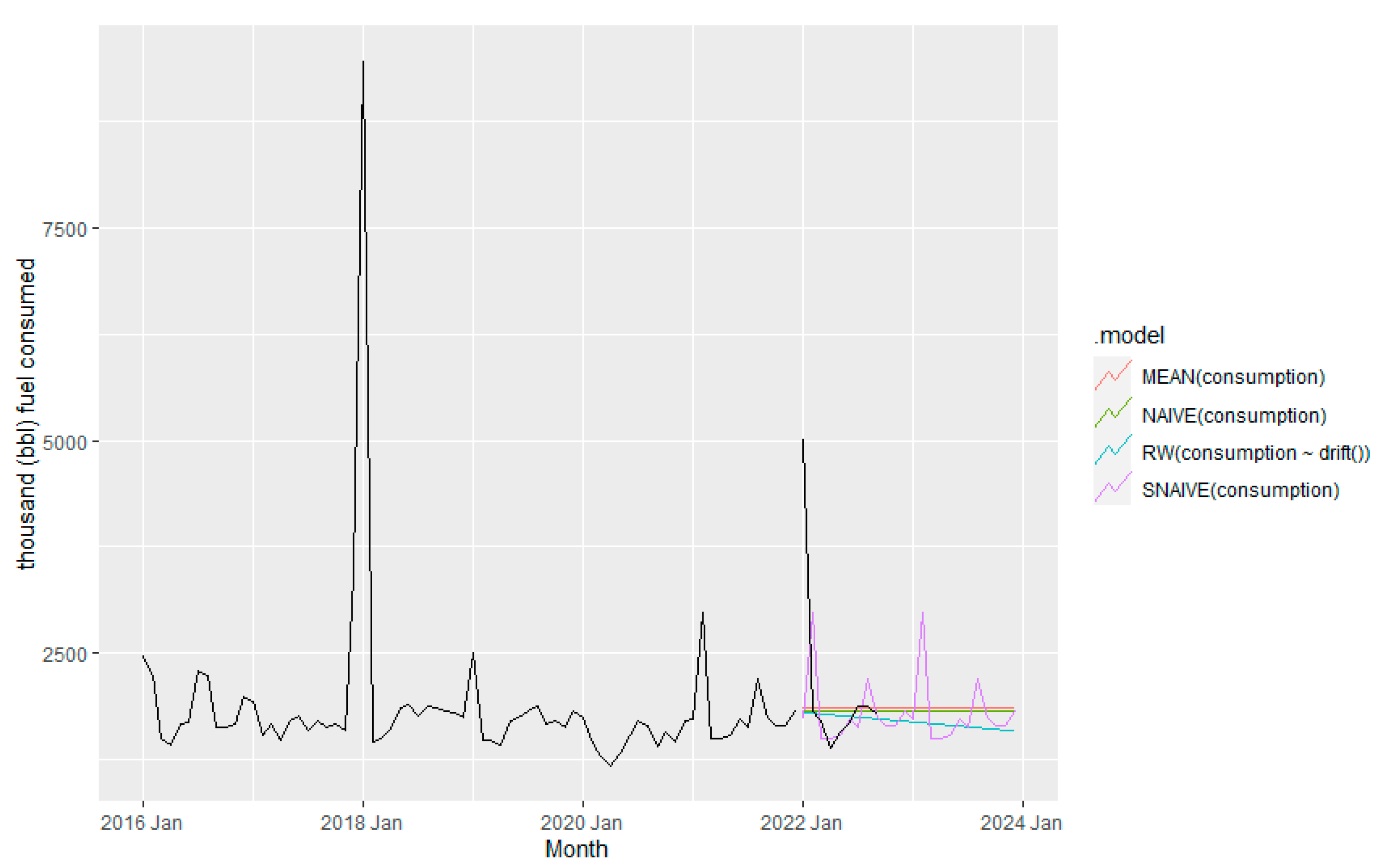
Figure 7 shows the results of the benchmark forecasting method. Based on
Figure 7, SNAIVE method can capture most of the fluctuation of fuel consumption and hence expected to provide comparable accurate prediction than other benchmark methods.
4.2. Forecasting of Fuel Consumption using the STL decomposition Methods
Decomposition techniques are used for finding and extracting the critical element of a time series. It can split the data into trends, seasonal or cyclical patterns. STL stands for Seasonal and Trend decomposition using Loess methods to perform additive decomposition of the data through a sequence of applications of the Loess smoother, which applies locally weighted polynomial regression at each point in the dataset. STL technique is resilience to outliers and is capable of handling seasonal time series with any seasonal frequency greater than one and is not restricted to either monthly or quarterly data (Thedosiou et al., 2011).
Figure 8 displays the STL method results.
4.3. Forecasting of Fuel Consumption using the ETS Methods
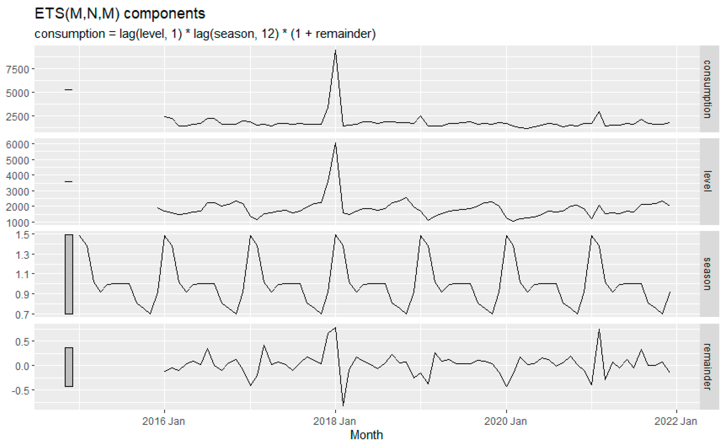
ETS is an acronym for Error, Trend, and Seasonal. It is a practical algorithm for datasets with seasonality and other prior assumptions about the data. ETS computes a weighted average over all observations in the input time series dataset as its prediction. ETS point forecasts are equal to the medians of the forecast distribution. In this study, the ETS (M, N, N) approach is implemented following the single exponential smoothing with multiplicative errors. For ETS models with multiplicative errors, the point forecasts will not be equal to the means of the forecast distributions.
The following ETS decomposition plot as shown in
Figure 9 has been obtained with a model (M, N, M) which stands for multiplicative (error), none (trend), and multiplicative (season) as best model in terms of AIC, AICc and BIC following the ETS () function of forecast package at R. it estimates the model parameters and returns information about the fitted model. The exponential smoothing parameters were observed as; α = 0.893 and ϒ = 0.0001. The σ2 is obtained as 0.0716. These parameters control the rate of change of the components; α and ϒ retain the flexibility of the level (error) and the trend, respectively. When α = 1, the level never updates (mean), and with ϒ=0 the seasonality is fixed (seasonal means).
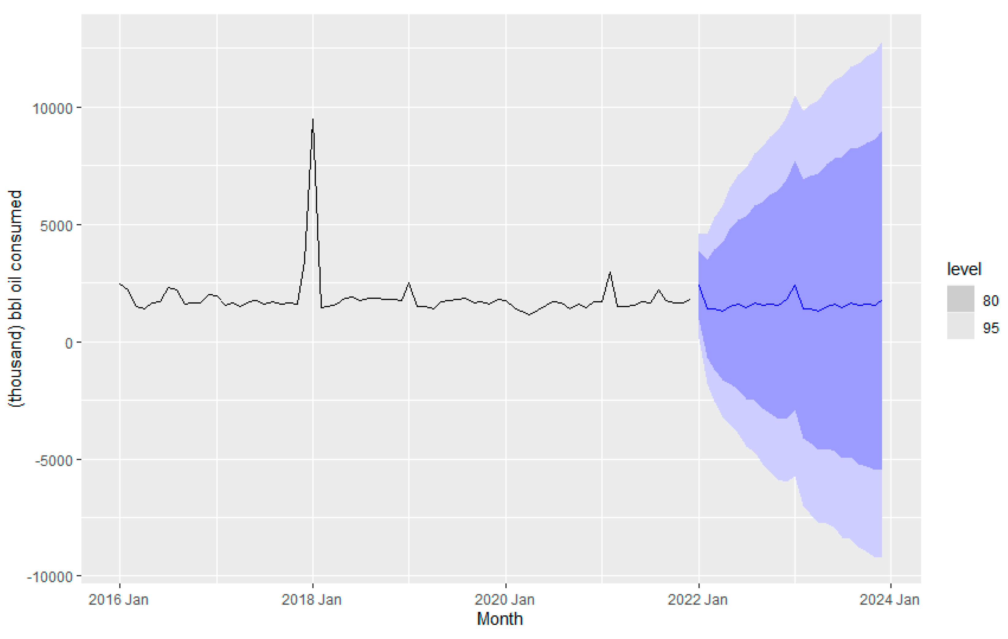
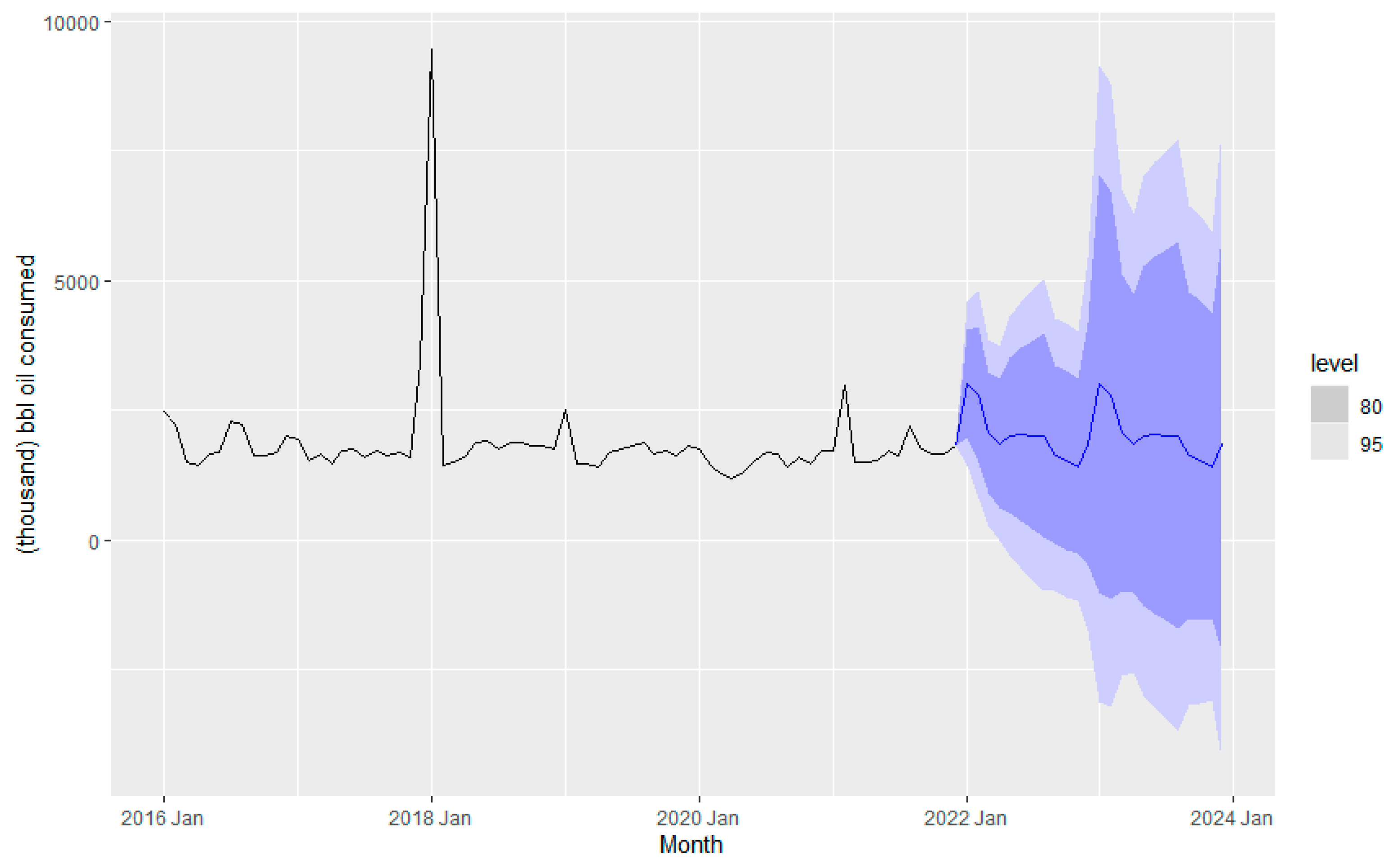
Figure 10 is consistent with the latter insights. The seasonality is not changing in the time series, and the level almost does not change.
Figure 10 depicts the forecasting of fuel consumption for a couple of years, from 2022 to 2024, using the ETS method. The level is the weighted average of previous observations, the season is the seasonality in the data, and the remainder is the data point that the model cannot predict (Rob J Hyndman and George Athanasopoulos).
4.4. Forecasting of Fuel Consumption using the ARIMA Method
ARIMA refers to "Autoregressive Integrated Moving Average". It is a forecasting approach based on previous observations assuming a dynamic correlation among the data points over time. The method combines autoregressive and moving average features. The first uses approaches; for instance, the current value is calculated considering the preceding value AR (1) or the previous two AR (2). The moving average calculates the average of different subsets of data points to smooth out the impact of outliers. ARIMA models forecast stationary times series refer that the properties do not relate to the time. (Equations 3 are used for the ARIMA model)
where
is the parameter for the
ith lag of the model. So, the model assumes that the data on the recent observation is influenced by the
p previous observations. The consumption data series has been checked by the Kwiatkowski-Phillips-Schmidt-Shin (KPSS) test [
10] () and found no differencing is required to make it stationary. ARIMA (
p, d, q); where p is the order of the autoregressive, d is the degree of first differencing and q is the order of the moving average part.
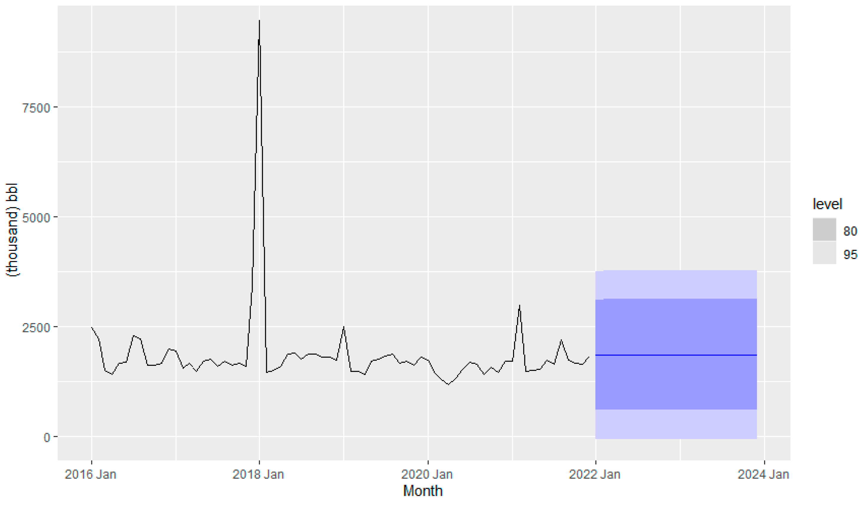
Figure 11 exhibits the ARIMA model predictions with just the first order of moving average.
Figure 11 exhibits the best suited ARIMA(p,d,q) model is ARIMA (0,0,1) using the
auto.arima() function in R obtained from variation of the Hyndman-Khandakar algorithm (Hyndman & Khandakar, 2008), which combines unit root tests, minimization of the AICc and MLE to obtain an ARIMA model.
4.5. Comparison of the Models in terms of Errors
Table 3 shows the error analysis of different applied forecast methods. The smallest value of RMSE has been observed for the ARIMA method with 953.74. The MAE and other error values were also the smallest for the ARIMA method to forecast fuel consumption.
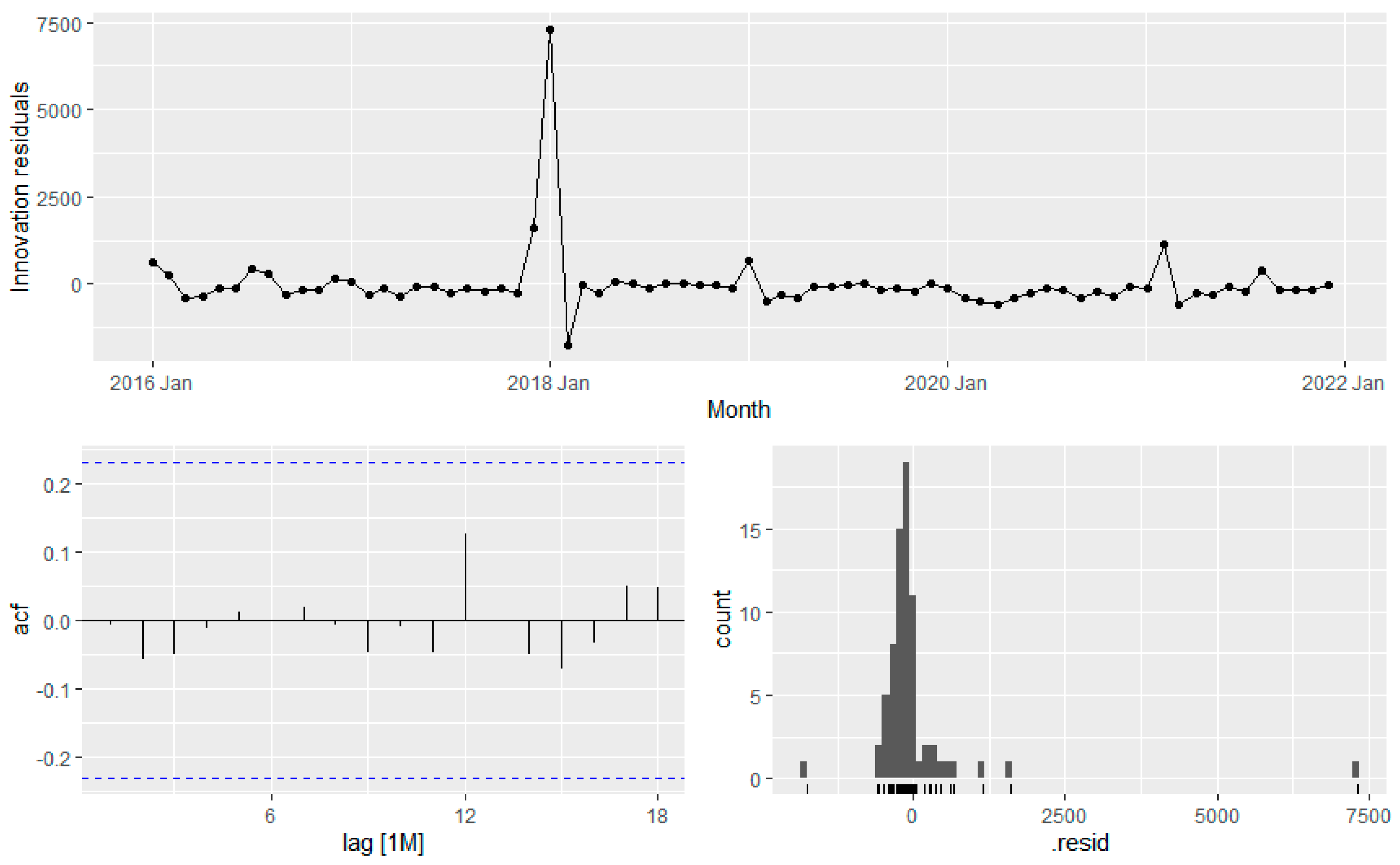
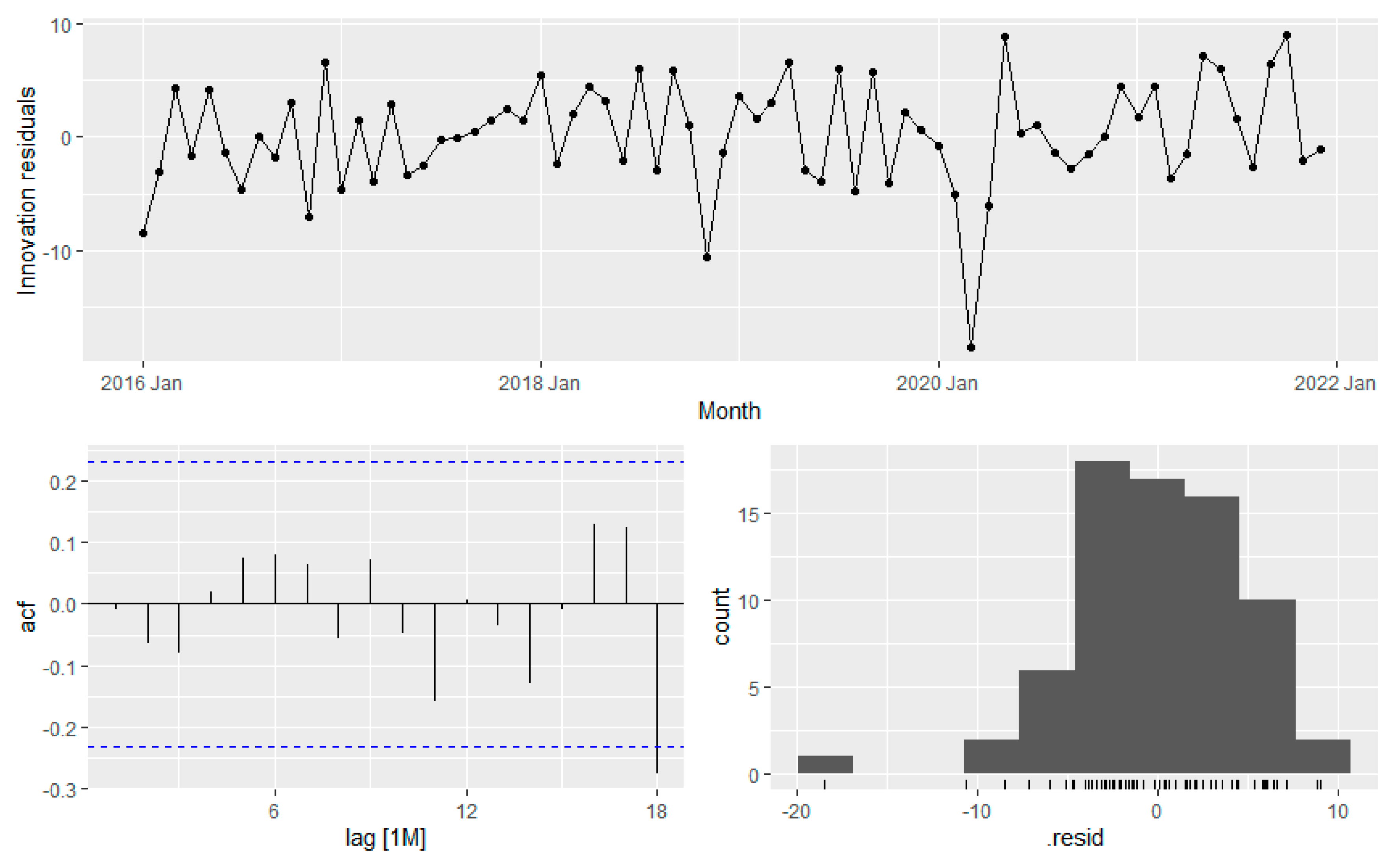
The residual plot in
Figure 12 shows a normal distribution that ensured the validity of the model without any significant interactions.
Also, The Ljung-Box test in table 4 shows that P-value is way higher than 0.05. So forecast model is good, and the residual does not contain any significant information.
Moreover, the accuracy is evaluated based on the test data set at
Table 5. The best forecasting method observed is ETS based on the RMSE value which is 799.59.
4.6. Forecasting of Fuel Consumption using the ARIMAX Method
An Autoregressive Integrated Moving Average with Explanatory variable (ARIMAX) is a multiple regression model which includes one or more autoregressive terms (AR) and/or one or more moving average (MA) term along with exogeneous variables. The model considers the interaction of multiple variables and uncertainty to generate a wider range of forecast model scenario. ARIMAX model is suitable for forecasting stationary or non-stationary data with any types of multivariate pattern; level or trend or seasonality or cyclicity. ARIMAX model allows to take the advantage of autocorrelation that may be present in residuals of the regression to improve the accuracy of the forecast. Therefore, ARIMAX model has been used here to capture the volatile and uncertain fuel consumption due to pandemic through integrating several exogeneous variables. The ARIMAX is described by Equation (4) as a common model for forecasting consumption time series.
where, Lt is the estimation of differenced consumption at time t.
is the autoregressive term with Pth order lag (AR (p) model).
is moving average term with qth order lag (MA (q)).
is the Ath exogenous variable term, and E is a constant value.
The p, d, and q orders for the ARIMAX model are determined from the Arima () function in the forecast R package. The Autoregressive Integrated Moving Average (ARIMA) model has been extended by incorporating exogenous variables (X) in the model and modified as ARIMAX using Bayesian framework. The exogenous variables chosen for the model are:
X1 = Mean monthly temperature in the U.S. from January 2016 to August 2022
X2 = Mean monthly petroleum fuel price in the U.S. from January 2016 to August 2022
X3= Mean monthly mileage traveled by vehicles in the U.S. from Jan 2016 to Aug 2022
The temperature variable was selected because it was observed that the pandemic is likely to be weak at high temperatures. Therefore, it has been considered a significant factor in understanding the impact of the pandemic on fuel consumption. Also, during the pandemic, the fuel price was volatile, and thus fuel consumption is likely to be affected by the price. Lastly, during the pandemic, people hardly traveled, reducing vehicle mileage; therefore, fuel consumption was also expected to decrease. Thus, in this model, all the seasonality has been eliminated from time series data. Then the model has been developed by interacting with one single variable, the combination of each two variables, and a combination of all three variables to find the best forecasting of the pandemic impact on fuel consumption. The temperature variable has been checked whether any first order differencing required or not using
KPSS test and found no differencing is required due to having P-value 0.1 (>0.5). Then the same data series has been checked whether any seasonal differencing is required or not using
KPSS test and found a seasonal differencing is required. Seasonal differencing with m =12 has been applied and the differenced data has been checked again using
KPSS test. The data series found converted to stationary and no further differencing was needed.
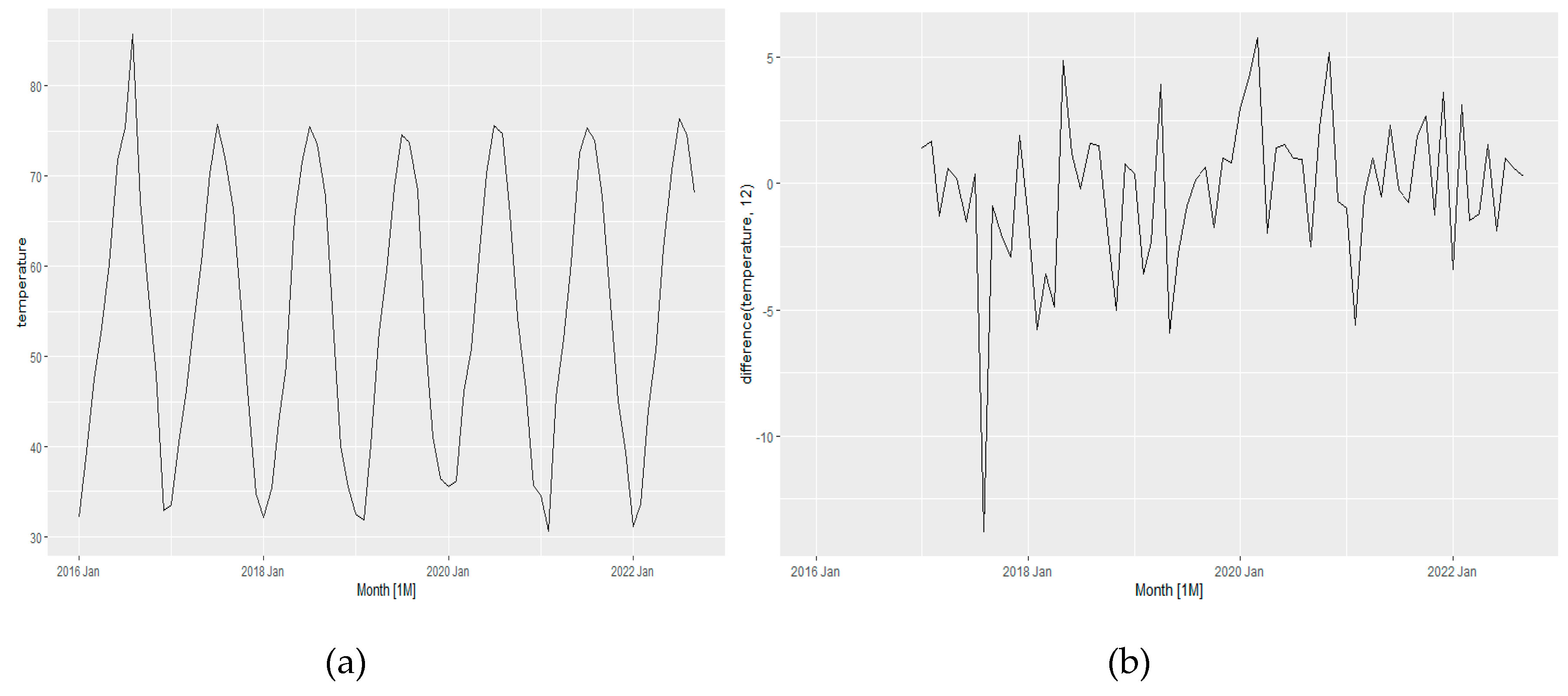
Figure 13 a shows the average temperature profile over seven years and
Figure 13b shows the differenced temperature variable which is converted into a stationary data and does not show any seasonality impacts.
The price variable has been checked whether any first order differencing is required or not using
KPSS test. We found that a first order differencing is required due to 0.01 p-value (<0.5). Then, the same data has been checked whether any seasonal differencing is required or not using
KPSS test and found no seasonal differencing is required. Therefore, a first order differencing has been applied and the differenced data has been checked again using
KPSS test. The data series found converted to stationery with p-value 0.1 and no further difference was needed.
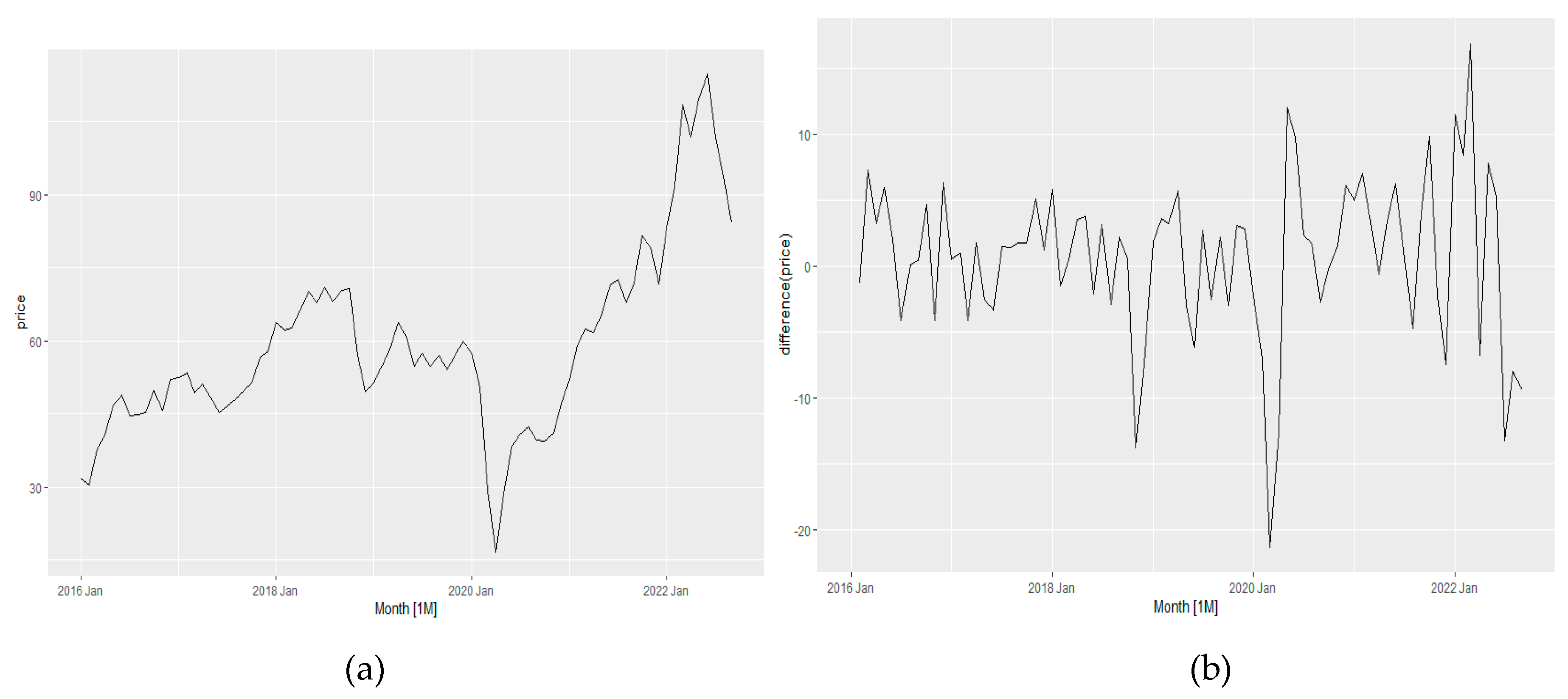
Figure 14a shows the seasonal impact of the price pattern and
Figure 14b shows the time series pattern after eliminating seasonal impact.
The miles variable has been checked whether any first order differencing required or not using KPSS test and found no differencing is required due to having P-value 0.1 (>0.5). Then the same data series has been checked whether any seasonal differencing is required or not using KPSS test and found a seasonal differencing is required. Seasonal differencing with m =12 has been applied and the differenced data has been checked again using KPSS test.
The data series found converted to stationery and no further difference was needed.
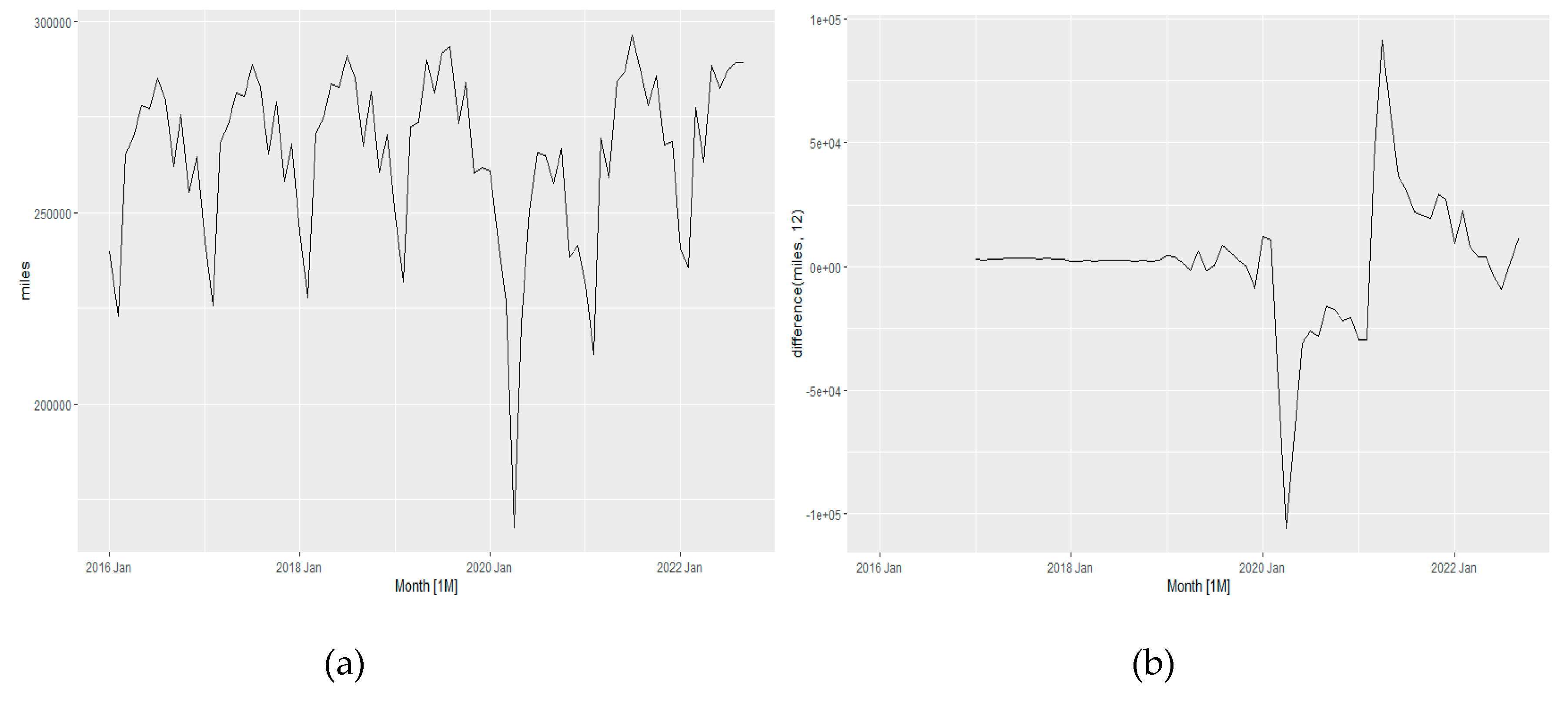
Figure 15 shows the differencing of miles variables over the seven years to convert into stationary data and eliminate any seasonality impacts.
So, all the variables have been converted to stationary data series. For consumption, there is no seasonal or first-order differencing required, confirmed by the KPSS and “unit_nseasonal” tests.
4.6.1. Analysis of fuel consumption forecast using combination of ARIMAX variables
The complete data set contains information of the associate variables for around seven years from January-2016 to September-2022. For the ARIMAX forecast model, the data set has been split into train dataset for five years from January-2016 to December-2020. The remaining data set has been used as a test data set. The accuracy has been estimated using the test dataset of consumption for the ARIMAX model using multiple interactions.
From
Table 6, the lowest RMSE is obtained from “price and temp” which is 735.62. Therefore, the forecast has been performed using the test data set consisting of observed price and temperature of 2021 and 2022 to predict the pandemic impact. The mileage seems to not have a significant contribution to fuel consumption.
The reason may be due to the home office during the lock-down period which leads to less travel and consequently less fuel consumption.
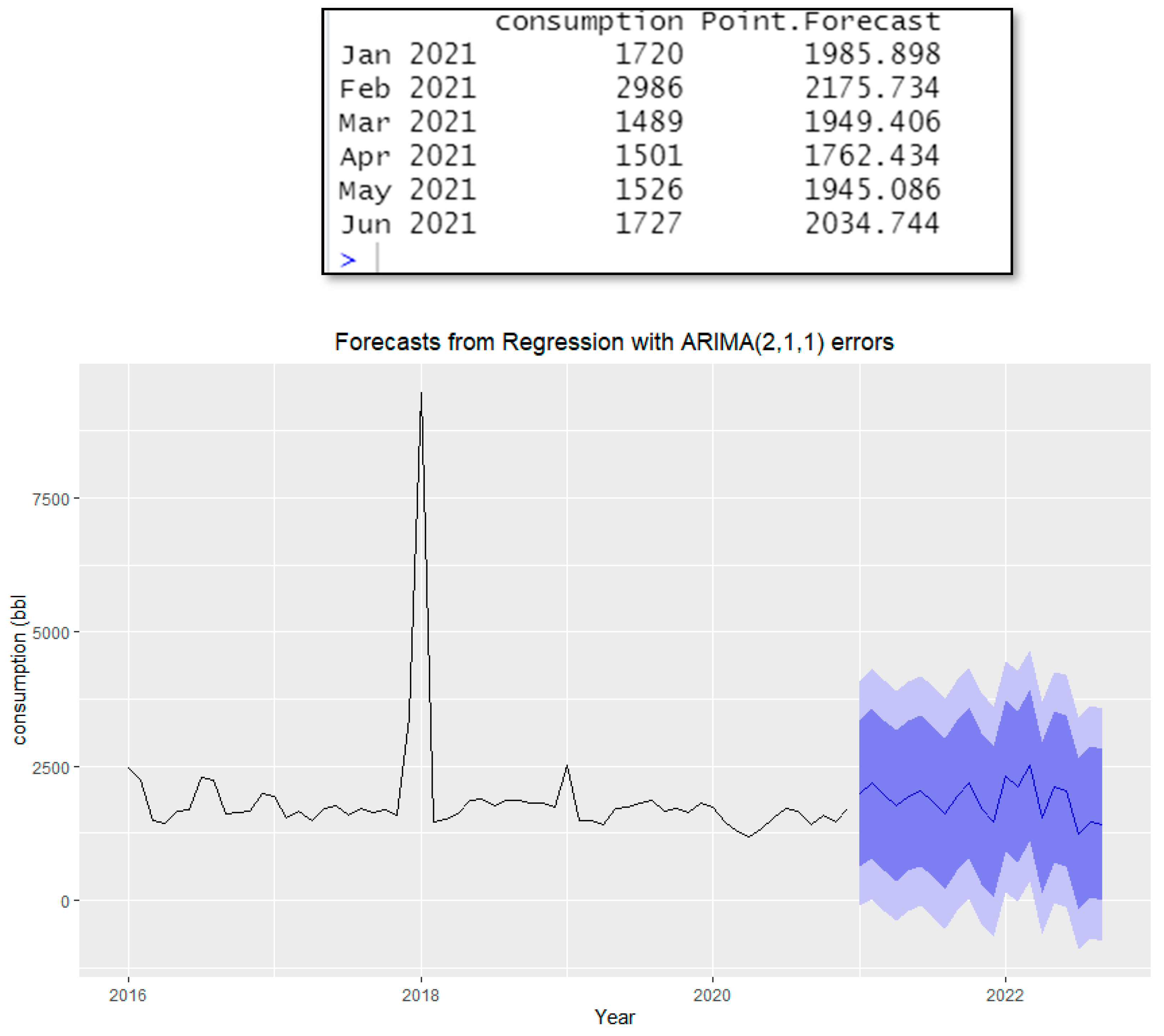
Figure 16 shows the forecasting of fuel consumption due to the impact of the pandemic and stochastic behavior.
5. Forecasting Model of Fuel Price
Petroleum price volatility highly influences the global economy. Hence, the price forecasting of this valuable commodity helps to mitigate the uncertainties associated to O&G industry. Price projections are critical to a variety of stakeholders. (Camp et. Al., 2020). All the forecasting models have been considered for the duration of two years from January-2022 to December-2023 for predicting fuel price.
5.1. Fuel Price Forecasting Using Benchmark Methods
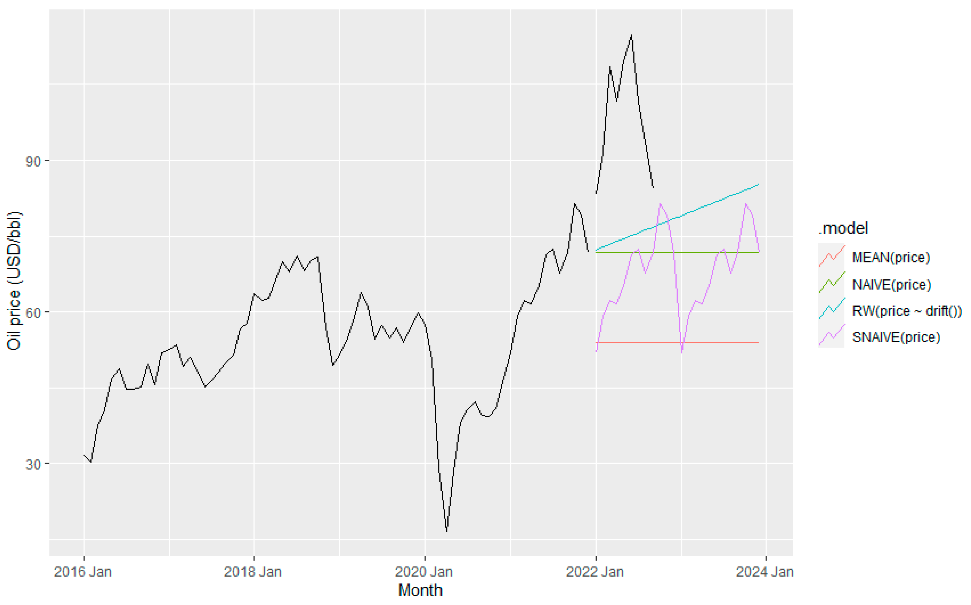
Figure 17 displays the forecasted values for the petroleum price in USA during 2022 using the Benchmark methods and data from 2016 to 2021 as the input for the model prediction.
5.2. Fuel Price Forecasting Using STL Methods
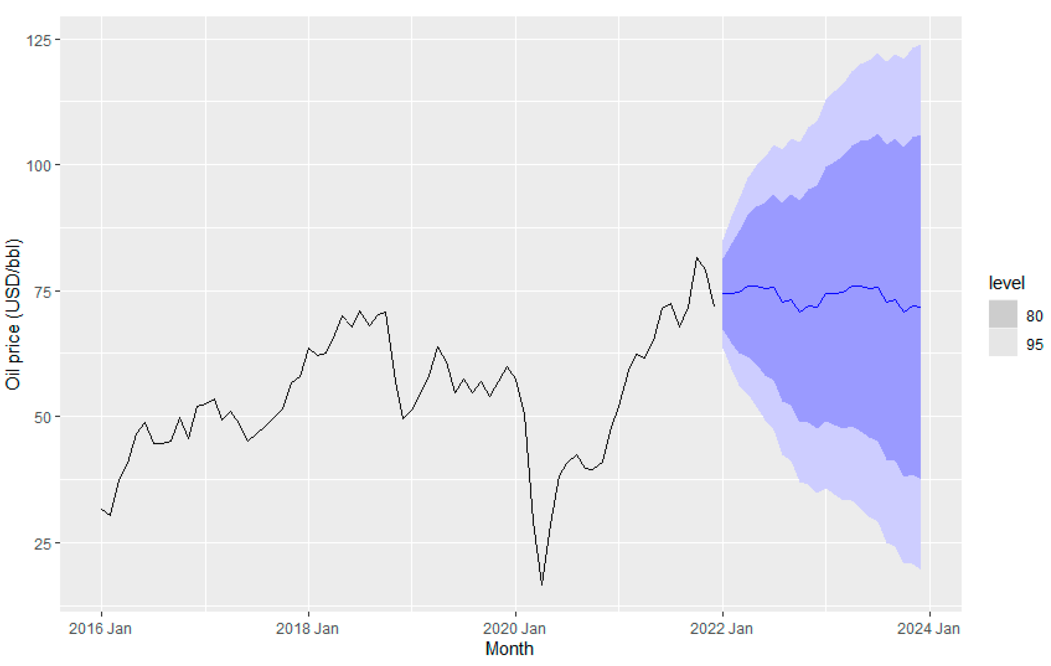
Figure 18 shows the STL decomposition model forecasts for the US oil price per barrel from 2022 to 2024, taking data from 2016 to 2021 as training data to feed the STL model.
5.3. Fuel Price Forecast Using ETS
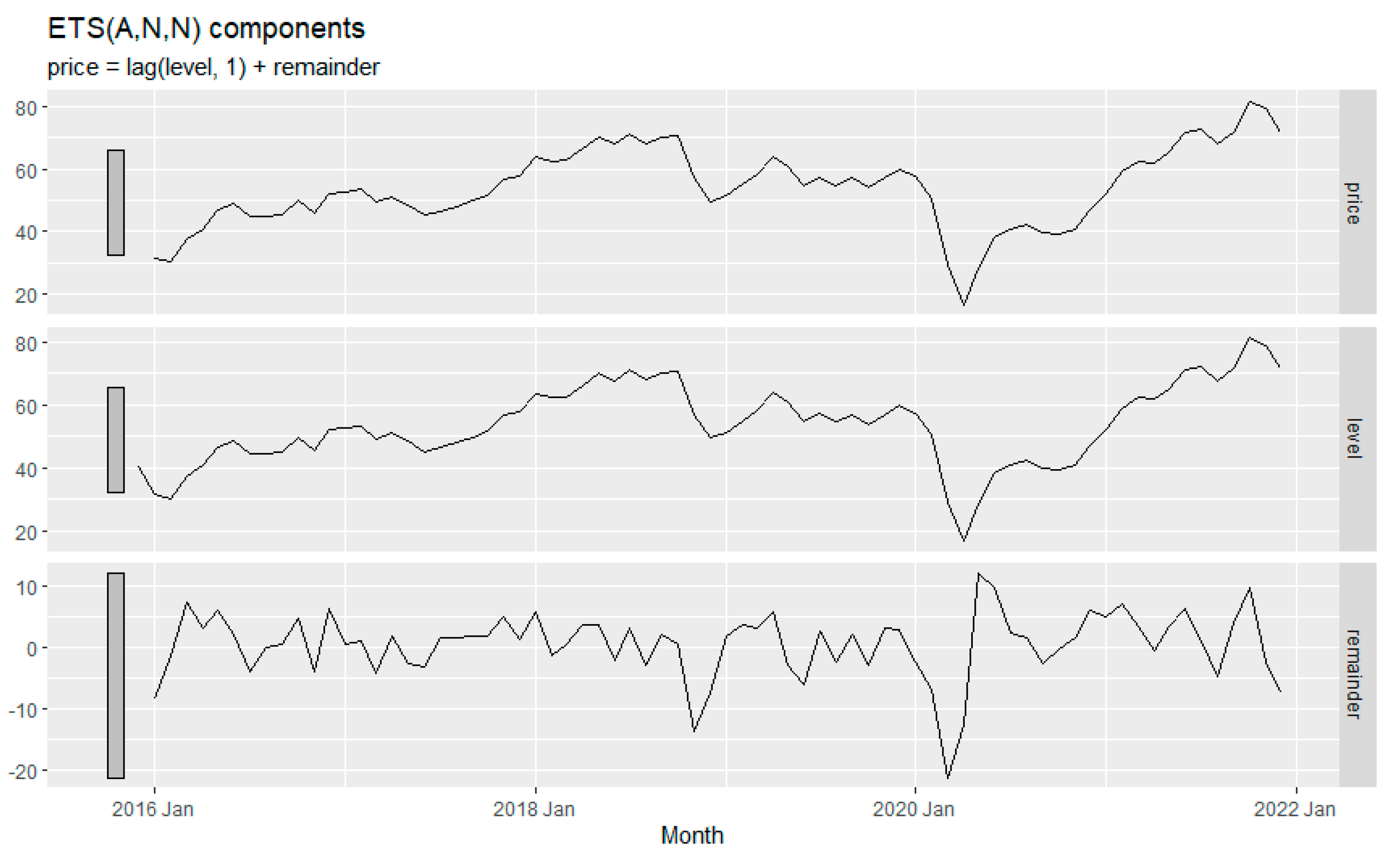
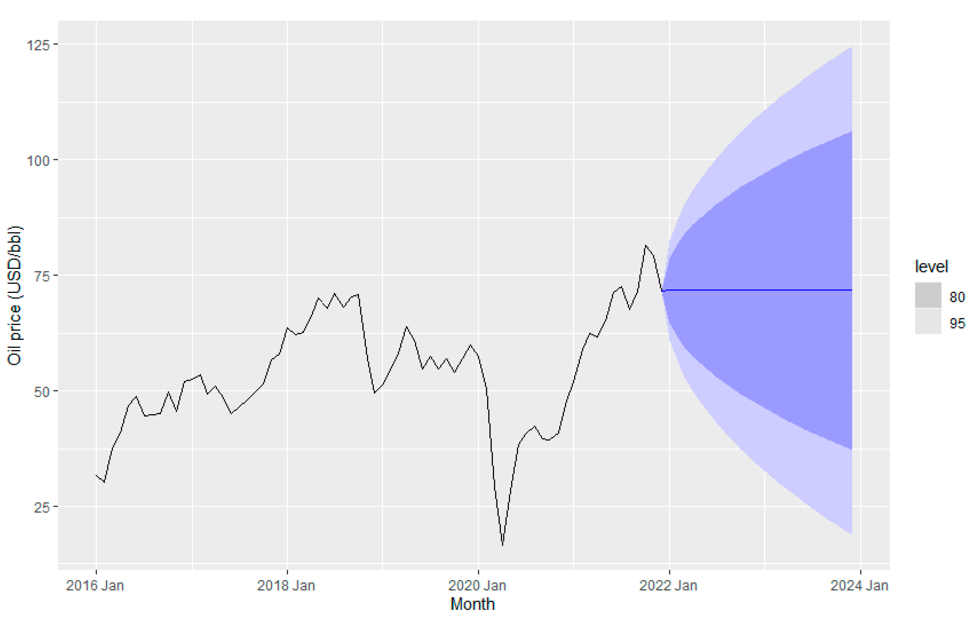
Figure 19 and
Figure 20 display the petroleum price implementing the ETS method. The ETS (A, N,N) approach has been obtained as the best model for fuel price prediction in terms of smallest AICc . In ETS (A, N,N), A refers to additive in error, and N is none either for trend and seasonality (Rob J Hyndman and Geoge Athanasopoulos). Oil price data do not have any trend or seasonal effects but seems to have cycling patterns.
5.4. Fuel Price Forecast Using ARIMA Method
Prior to applying ARIMA method, the KPSS test for price data has been implemented to check the stationarity of data and a P-value of 0.01 was found which is significant. Therefore, a first-order differencing has been applied to the price data, and it is found that the data is stationary. No seasonal differencing was needed as the data set had already been converted to stationary after first-order differencing.
Figure 21. The best Model obtained was ARIMA (1,0,1) (0,0,1) [
12] with σ
2 23.19 with 439.55 AIC, and 440.46 AICc.
5.5. Comparison of the Models in terms of Errors
Table 7 shows the results of error calculated from the training data set for all seven models analyzed before forecasting the fuel price.
The ARIMA method provides the lowest forecast error as shown in
Table 7.
Figure 22 shows the residual and Ljung-Box test result as shown in
Table 8 ensure the model integrity. The residual analysis shows the residual looks like white noise with no significant autocorrelation.
A comparison of different forecasting models for fuel price is shown in
Table 9.
5.6. Fuel Price Forecast Using ARIMAX Method
We use the ARIMAX technique to forecast fuel consumption. The data is checked for stationary, and then is transformed to non-stationary data to eliminate any seasonal impact. Then, the results of ARIMA model are shown in
Table 10 which includes various combinations of exogenous variables to forecast price using the test data. In addition,
Table 10 shows the parameters of the ARIMA errors.
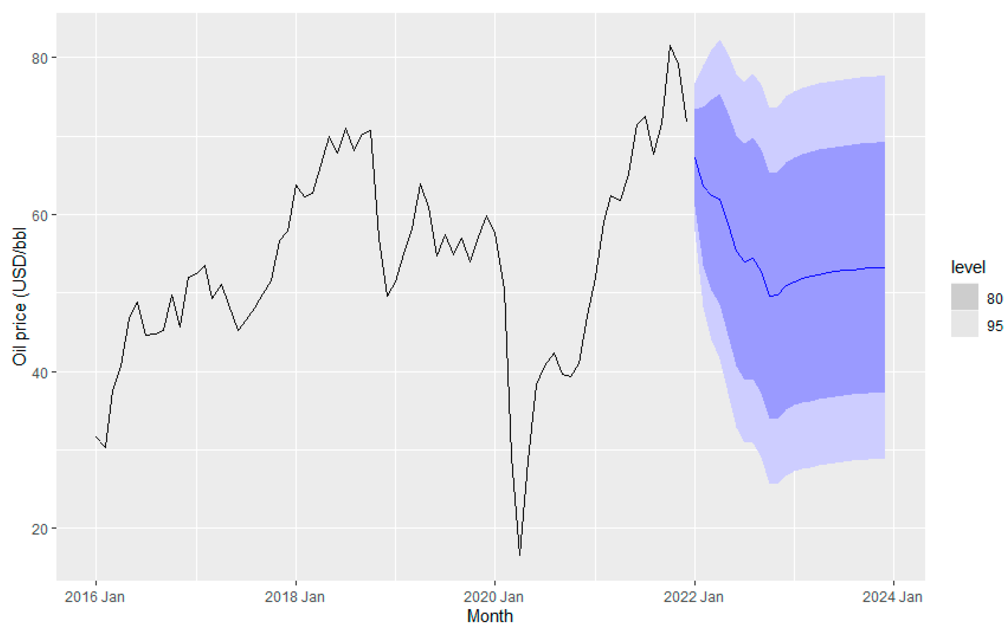
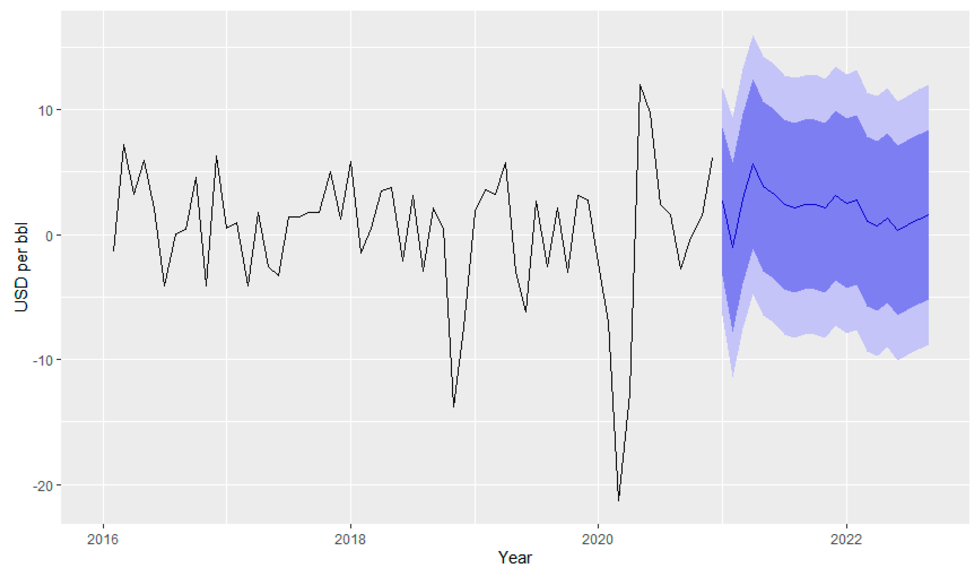
It is observed that there is no significant improvement in variable elimination in terms of minimizing errors. However, the ARIMAX model with ARIMA (0,0,1) errors with consumption and milage variables gives comparatively less RMSE error. It also indicates that temperature does not change the fuel price significantly. Therefore, the ARIMAX model with ARIMA (0,0,1) errors and two variables is considered for forecasting the fuel price. The fuel price forecasts obtained from this ARIMAX model are plotted in
Figure 23.
6. Result and Discussion
6.1. Synopsis of Pandemic Impact on Fuel Price.
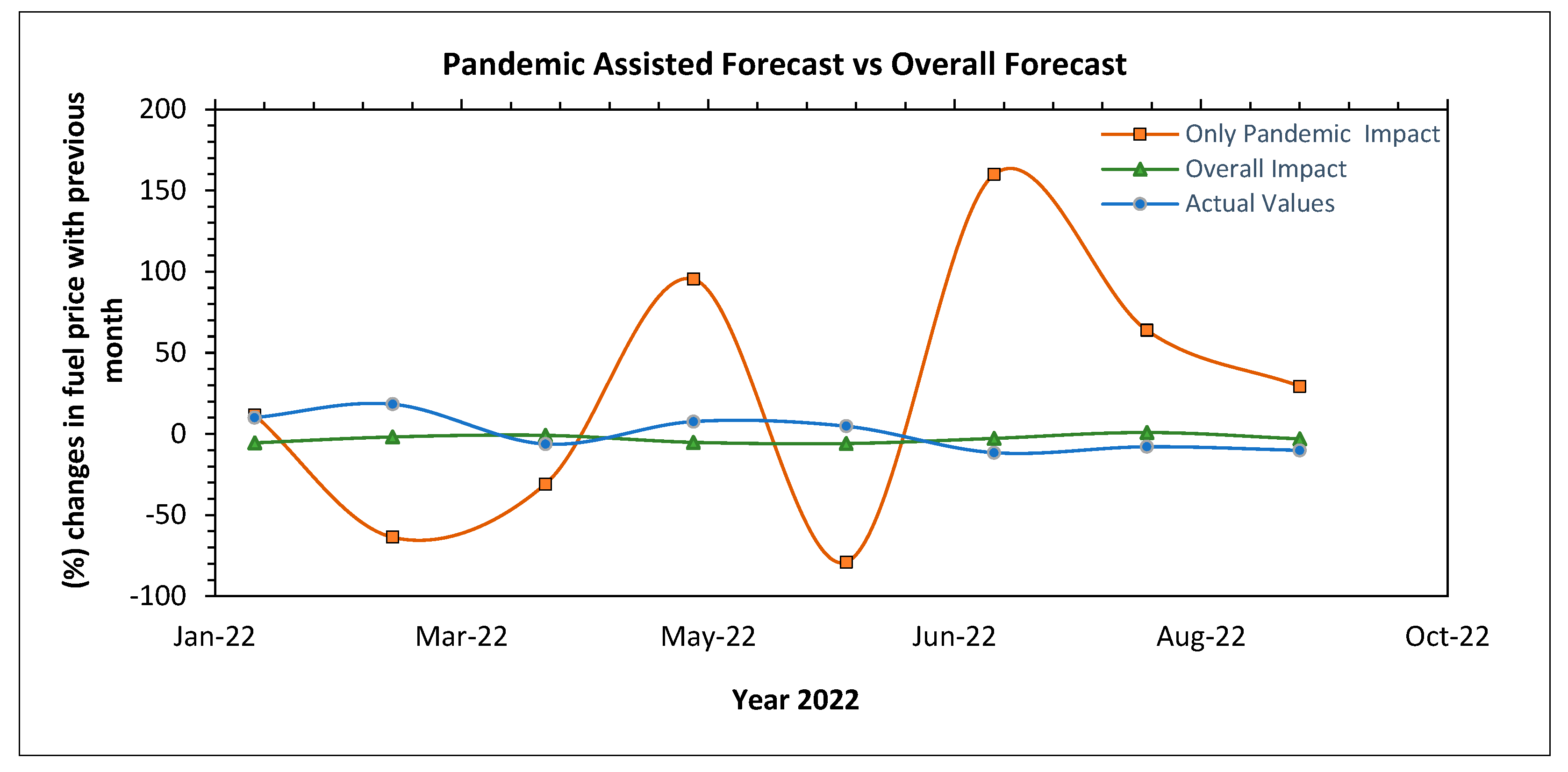
Figurer 24 displays the percentage change pattern of each month’s fuel price with respect to previous month for eight months from January 2022 to August 2022. The reason behind considering the percentage change of fuel price instead of actual price values is that the price data were differenced to obtain stationary data for ARIMAX modeling. Therefore, a percentage change price estimation ensures that the homogeneous comparison of how far the predicted values are from actual values in various scenarios. In
Figure 24, three sets of values for fuel price change (%) have been considered. The first set comprises of the actual observed changes of fuel price in year 2022 from January to August which was considered as test set and kept aside from the trained model. The second set of price value difference (%) was the prediction value obtained from the best performing forecast model. The ARIMA model was considered as the most accurate among all seven models evaluated in terms of error metrics and discussed in
Table 7. ARIMA model has taken into account both seasonal and pandemic impact to forecast the fuel price. Hence, the values of fuel price change obtained from ARIMA method has been considered as the overall impact where pandemic was not excluded from weather and seasonal impact. The third set of value for fuel price change was obtained from ARIMAX method. Here all the abnormal fluctuations on fuel price due to pandemic impact was isolated by removing the seasonal influence through seasonal differencing. Furthermore, three exogeneous variables;
temperature, consumption, and mileage travelled were included into ARIMAX model considering high impactful on fuel price during the pandemic period.
Figure 24 also shows abrupt fluctuation when only the pandemic was considered for forecasting; this shape is expected when another chaotic event such as the COVID-19 outbreak appears.
6.2. Synopsis of Pandemic Impact on Fuel Consumption
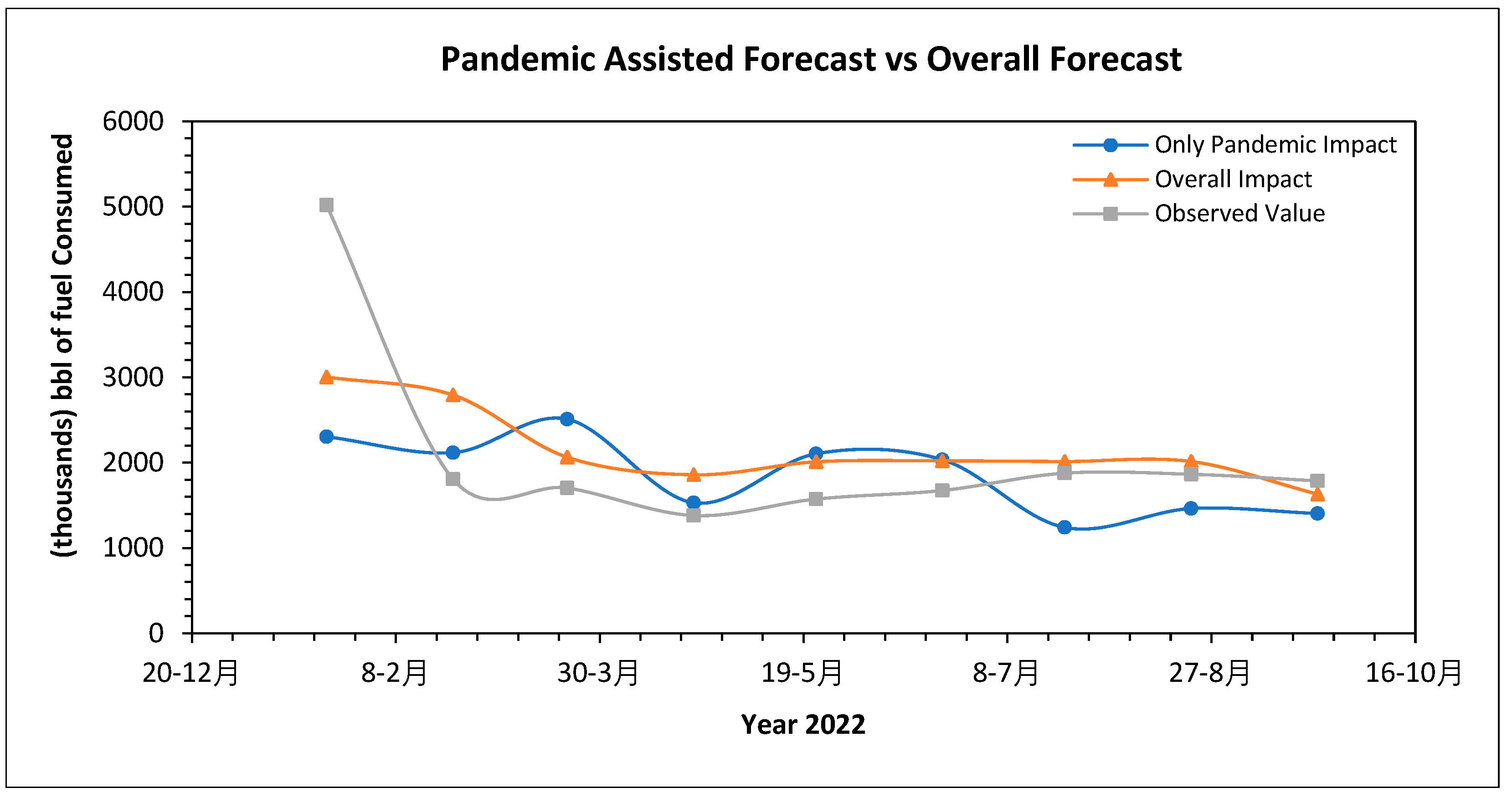
Figure 25 illustrates the three identical scenarios considered for change of fuel price at section 6.1. Observed values of consumption were extracted from the test data set. Consumption for only pandemic influence has been obtained by ARIMAC method through removing seasonal and weather impact. The overall impact indicated the forecast of consumption pattern where all the influential factors; (pandemic, season, etc.) were included and the best suited model selected for overall impact was ETS compared to seven other models. Here, three scenarios are established: pandemic impact, overall impact, and actual data. Considering the overall impact, the curve behaves more like the observed values, which aligns with the ideas presented in this paper. When only the pandemic is considered, the curve shape falls abruptly, missing the data pattern.
7. Conclusions
The pandemic has much more impact on fuel prices than consumption. The article will help to predict a rudimentary assessment of future year fuel consumption and cost in both cases of the presence or absence of any pandemic. A pandemic or any outbreak results in a much more volatile and stochastic pattern in energy trends. The analysis can be further extended and modified by including more exogenous variables, such as production size, number of industries using petroleum fuel, and more breakdown of the pandemic period: weekly, hourly and half-hourly. The government and industry can get a rudimentary assumption from this article to understand the forecast of fuel consumption and fuel price based on overall weather, seasonal change, and other stochastic irregular impact. Also, the authority can optimize the operation and production in case of any outbreak appears which comes with most stochasticity following the second part of the article. That will help to prepare in advance and adjust the plan with minimal or no loss of money and economy.
Author Contributions
Conceptualization, A.N.S.; methodology, A.N.S; software, A.N.S.; validation, A.N.S., T.R; formal analysis, A.N.S.; investigation, A.N.S.; resources, A.N.S.; writing—original draft preparation, A.N.S., M.H.B; writing—review and editing, T.R., M.H.B; visualization, supervision, A.N.S.; project administration, A.N.S., M.H.B. All authors have read and agreed to the published version of the manuscript.
Funding
This research received no external funding.
Data Availability Statement
Not applicable.
Acknowledgments
Not applicable.
Conflicts of Interest
The authors declare no conflict of interest.
References
- Agdas D, Barooah P. Impact of the COVID-19 Pandemic on the U.S. Electricity Demand and Supply: An Early View From Data. IEEE Access. 2020 Aug 17;8:151523-151534. [CrossRef]
- Alasali, F., Haben, S., Becerra, V. et al. Day-ahead industrial load forecasting for electric RTG cranes. J. Mod. Power Syst. Clean Energy 6, 223–234 (2018). [CrossRef]
- E.F. Sánchez-Úbeda, J. Portela, A. Muñoz, E. Chueca Montuenga, M. Hallack, Impact of COVID-19 on electricity demand of Latin America and the Caribbean countries, Sustainable Energy, Grids and Networks, Volume 30, 2022, 100610, ISSN 2352-4677. [CrossRef]
- Kevin M. Camp, David Mead, Stephen B. Reed, Christopher Sitter, and Derek Wasilewski, "From the barrel to the pump: the impact of the COVID-19 pandemic on prices for petroleum products," Monthly Labor Review, U.S. Bureau of Labor Statistics, October 2020. [CrossRef]
- üngör, Oray and Ertugrul, Hasan Murat and Soytas, Ugur, The Impact of COVID-19 Outbreak on Turkish Gasoline Consumption (May 27, 2020). Available at https://ssrn.com/abstract=3611788.
- Ou, S., He, X., Ji, W. et al. Machine learning model to project the impact of COVID-19 on US motor gasoline demand. Nat Energy 5, 666–673 (2020). [CrossRef]
- L. Vanessa Smith, Nori Tarui, Takashi Yamagata, Assessing the impact of COVID-19 on global fossil fuel consumption and CO2 emissions, Energy Economics, Volume 97, 2021, 105170, ISSN 0140-9883. [CrossRef]
- Zhang X, Li Z, Wang J. Impact of COVID-19 pandemic on energy consumption and carbon dioxide emissions in China's transportation sector. Case Studies in Thermal Engineering. 2021 Aug;26:101091. Epub 2021 May 24. https://www.eia.gov/electricity/data.php. [CrossRef]
- Denis Kwiatkowski, Peter C.B. Phillips, Peter Schmidt, Yongcheol Shin , ‘Testing the null hypothesis of stationarity against the alternative of a unit root: How sure are we that economic time series have a unit root?’; Journal of Econometrics Volume 54, Issues 1–3, October–December 1992, Pages 159-178.
- Feras Alasali; Khaled Nusair; Lina Alhmoud; Eyad Zarour. Impact of the COVID-19 Pandemic on Electricity Demand and Load Forecasting’. Sustainability 2021, 13(3), 1435. [CrossRef]
- Baker, S.; Bloom, N.; Davis, S.; Terry, S. COVID-induced economic uncertainty. Natl. Bur. Econ. Res. Pap. 2020. [Google Scholar]
- Abu-Rayash, A.; Dincer, I. Analysis of the electricity demand trends amidst the COVID-19 coronavirus pandemic. Energy Res. Soc. Sci. 2020, 68, 101682. [Google Scholar] [CrossRef] [PubMed]
- Indre Siksnelyte-Butkiene. Impact of the COVID-19 Pandemic to the Sustainability of the Energy Sector. Sustainability 2021, 13(23), 12973. [CrossRef]
- Vijay Kotu, Bala Deshpande. Time Series Forecasting, Data Science (Second Edition), 2019.
- Soumik Ray1*, Banjul Bhattacharyya. STATISTICAL MODELING AND FORECASTING OF ARIMA AND ARIMAX MODELS FOR FOOD GRAINS PRODUCTION AND NET AVAILABILITY OF INDIA. Journal of Experimental Biology and Agricultural Sciences, ISSN No. 2320 – 8694, 2020.
- Hee-Jeong Kim; Ju-Hyung Kim; Jin-bin Im. Forecasting Offline Retail Sales in the COVID-19 Pandemic Period: A Case Study of a Complex Shopping Mall in South Korea, Buildings 2023, 13(3), 627. [CrossRef]
- Jain, G.; Mallick, B.; A Study of Time Series Models ARIMA and ETS. Available at SSRN 2898968. 2017. Available online: https://www.mecs-press.org/ijmecs/ijmecs-v9-n4/IJMECS-V9-N4-7.pdf (accessed on 30 June 2017).
- Sung-Eun Kang; Changyeon Park; Choong-Ki Lee 2; Seunghoon Lee. The Stress-Induced Impact of COVID-19 on Tourism and Hospitality Workers, Sustainability 2021, 13(3), 1327. [CrossRef]
Figure 1.
Petroleum Fuel Consumption in the USA for Power Generation.
Figure 1.
Petroleum Fuel Consumption in the USA for Power Generation.
Figure 2.
Comparison of monthly petroleum fuel consumption from 2016 to 2022 (a) Comparison of monthly petroleum fuel consumption from 2016 to2022; (b) Seasonality analysis of monthly petroleum fuel consumption from 2016 to 2022.
Figure 2.
Comparison of monthly petroleum fuel consumption from 2016 to 2022 (a) Comparison of monthly petroleum fuel consumption from 2016 to2022; (b) Seasonality analysis of monthly petroleum fuel consumption from 2016 to 2022.
Figure 3.
ACF and PACF plot of monthly fuel consumption.
Figure 3.
ACF and PACF plot of monthly fuel consumption.
Figure 4.
Petroleum Fuel Price from 2016 to 2022.
Figure 4.
Petroleum Fuel Price from 2016 to 2022.
Figure 5.
Comparison of monthly petroleum fuel price from 2016 to 2022 (a) Comparison of monthly petroleum fuel price from 2016 to 2022 (b) Seasonality analysis of monthly petroleum fuel price from 2016 to 2022.
Figure 5.
Comparison of monthly petroleum fuel price from 2016 to 2022 (a) Comparison of monthly petroleum fuel price from 2016 to 2022 (b) Seasonality analysis of monthly petroleum fuel price from 2016 to 2022.
Figure 6.
PACF and ACF plot of fuel price from 2016 to 2022.
Figure 6.
PACF and ACF plot of fuel price from 2016 to 2022.
Figure 7.
Forecast of fuel consumption using the benchmark methods.
Figure 7.
Forecast of fuel consumption using the benchmark methods.
Figure 8.
Forecast of fuel consumption for 2022 and 2024 using the STL decomposition method.
Figure 8.
Forecast of fuel consumption for 2022 and 2024 using the STL decomposition method.
Figure 9.
ETS decomposition plot of fuel consumption.
Figure 9.
ETS decomposition plot of fuel consumption.
Figure 10.
Forecast of Fuel Consumption using the ETS decomposition method.
Figure 10.
Forecast of Fuel Consumption using the ETS decomposition method.
Figure 11.
Forecast of fuel consumption using ARIMA (0,0,1) method.
Figure 11.
Forecast of fuel consumption using ARIMA (0,0,1) method.
Figure 12.
Residual analysis of ARIMA forecasting method.
Figure 12.
Residual analysis of ARIMA forecasting method.
Figure 13.
The mean temperature profile of seven years with seasonality.
Figure 13.
The mean temperature profile of seven years with seasonality.
Figure 14.
Monthly average price before and after differencing over seven years.
Figure 14.
Monthly average price before and after differencing over seven years.
Figure 15.
Monthly mean of mileage data series before and after differencing over seven years.
Figure 15.
Monthly mean of mileage data series before and after differencing over seven years.
Figure 16.
Consumption forecast using the ARIMA (2,1,1) model.
Figure 16.
Consumption forecast using the ARIMA (2,1,1) model.
Figure 17.
Benchmark methods for price forecasting.
Figure 17.
Benchmark methods for price forecasting.
Figure 18.
Forecasting of petroleum fuel price using STL decomposition Model.
Figure 18.
Forecasting of petroleum fuel price using STL decomposition Model.
Figure 19.
Decomposition results using ETS(A,N,N).
Figure 19.
Decomposition results using ETS(A,N,N).
Figure 20.
Forecasting of petroleum fuel price at 2022 using ETS (A, N,N) decomposition Model.
Figure 20.
Forecasting of petroleum fuel price at 2022 using ETS (A, N,N) decomposition Model.
Figure 21.
ARIMA model results for forecasting the oil price.
Figure 21.
ARIMA model results for forecasting the oil price.
Figure 22.
Residual analysis of ARIMA model for fuel price forecasting.
Figure 22.
Residual analysis of ARIMA model for fuel price forecasting.
Figure 23.
Forecasted fuel price using the ARIMAX method with ARIMA(0,0,1) error.
Figure 23.
Forecasted fuel price using the ARIMAX method with ARIMA(0,0,1) error.
Figure 24.
Comparison of prediction in fuel price changes for different schemes.
Figure 24.
Comparison of prediction in fuel price changes for different schemes.
Figure 25.
Changes in oil consumption prediction for different schemes.
Figure 25.
Changes in oil consumption prediction for different schemes.
Table 1.
Petroleum fuel consumption (thousands bbl) between 2016 and 2022.
Table 1.
Petroleum fuel consumption (thousands bbl) between 2016 and 2022.
| |
Pre-COVID |
COVID |
Post - COVID |
| |
2016 |
2017 |
2018 |
2019 |
2020 |
2021 |
2022 |
| Max. Consumption |
2,472 |
3,414 |
9,468 |
2,506 |
1,741 |
3,367 |
5,452 |
| Min Consumption |
1,421 |
1,749 |
1,451 |
1,417 |
1,169 |
1,360 |
1,306 |
| Avg. Consumption |
1,867 |
1,808 |
2,385 |
1,736 |
1,501 |
1,723 |
2,102 |
| The (%) change in consumption in pre- and post-pandemic years with reference 2020 |
| |
2016 |
2017 |
2018 |
2019 |
2020 |
2021 |
2022 |
| Max. Consumption |
29 |
49 |
81 |
30 |
- |
48 |
68 |
| Min Consumption |
17 |
33 |
19 |
17 |
- |
14 |
10 |
| Avg. Consumption |
19 |
16 |
37 |
13 |
- |
12 |
28 |
Table 2.
Summary of the petroleum fuel price between 2016 and 2022.
Table 2.
Summary of the petroleum fuel price between 2016 and 2022.
| |
2016 |
2017 |
2018 |
2019 |
2020 |
2021 |
2022 (Aug) |
| Max. Price |
51.97 |
57.88 |
70.98 |
63.86 |
57.52 |
81.48 |
114.84 |
| Min Price |
30.92 |
45.18 |
49.52 |
51.38 |
16.55 |
52.01 |
83.22 |
| Avg. Price |
43.15 |
50.88 |
64.94 |
56.98 |
39.23 |
67.99 |
97.66 |
| The (%) change in ($) in pre- and post-pandemic years with year 2020 |
| |
2016 |
2017 |
2018 |
2019 |
2020 |
2021 |
2022 (Aug) |
| Max. Price |
-10% |
0.62% |
18% |
10% |
- |
29% |
50% |
| Min Price |
46% |
63% |
66% |
67% |
- |
68% |
80% |
| Avg. Price |
9% |
22% |
39% |
31% |
- |
42% |
59% |
Table 3.
Comparison of error analysis of different applied forecast methods.
Table 3.
Comparison of error analysis of different applied forecast methods.
| Train Data |
Model |
ME |
RMSE |
MAE |
MPE |
MAPE |
MASE |
RMSSE |
ACF1 |
| MEAN |
1.01E-13 |
968.86 |
374.49 |
-8.19 |
16.59 |
0.75 |
0.69 |
0.16 |
| NAIVE |
-9.30 |
1260.73 |
428.71 |
-8.08 |
21.20 |
0.86 |
0.90 |
-0.36 |
| SNAIVE |
-12.88 |
1391.16 |
497.48 |
-6.55 |
20.03 |
1 |
1 |
0.19 |
| Drift |
7.69E-14 |
1260.6 |
429.36 |
-7.53 |
21.20 |
0.86 |
0.90 |
-0.36 |
| STL |
-2.81 |
1236.83 |
429.86 |
-7.62 |
20.66 |
0.86 |
0.88 |
-0.39 |
| ETS |
-37.51 |
1038.48 |
413.12 |
-6.85 |
21.30 |
0.83 |
0.74 |
-0.29 |
| ARIMA |
-1.27 |
953.74 |
366.56 |
-8.12 |
16.37 |
0.736 |
0.68 |
-0.007 |
Table 4.
Ljung-Box test results for ARIMA forecast to forecast energy consumption.
Table 4.
Ljung-Box test results for ARIMA forecast to forecast energy consumption.
| Model |
Statistic |
P-value |
| ARIMA |
0.705 |
0.998 |
Table 5.
Consumption forecast on TEST data.
Table 5.
Consumption forecast on TEST data.
| Test Data |
Model |
ME |
RMSE |
MAE |
MPE |
MAPE |
MASE |
RMSSE |
ACF1 |
| MEAN |
227.83 |
1074.67 |
486.20 |
-1.14 |
15.70 |
0.98 |
0.77 |
0.03 |
| NAÏVE |
266.78 |
1083.60 |
473.22 |
0.99 |
14.66 |
0.95 |
0.78 |
0.03 |
| Drift |
313.33 |
1084.76 |
477.20 |
3.65 |
14.67 |
0.96 |
0.78 |
0.02 |
| SNAIVE |
242.33 |
1178.66 |
614.56 |
0.33 |
21.27 |
1.24 |
0.85 |
-0.34 |
| STL |
494.23 |
908.46 |
494.23 |
17.29 |
17.29 |
0.99 |
0.65 |
0.07 |
| ETS |
-79.71 |
799.59 |
561.94 |
-13.85 |
24.70 |
1.13 |
0.57 |
-0.23 |
| ARIMA |
226.63 |
1074.89 |
486.83 |
-1.21 |
15.74 |
0.98 |
0.77 |
0.03 |
Table 6.
Fuel Consumption result analysis.
Table 6.
Fuel Consumption result analysis.
| Variables |
ME |
RMSE |
MAE |
MPE |
MAPE |
ARIMA Model |
| Price, Miles & Temp |
333.069 |
857.391 |
450.462 |
10.451 |
17.818 |
ARIMA(2,1,0) |
| Price & Temp |
48.017 |
735.620 |
512.370 |
-4.54 |
24.00 |
ARIMA(2,1,1) |
| Price |
2.99 |
736.492 |
476.701 |
-5.92 |
21.77 |
ARIMA(0,0,0) |
| Temp & Miles |
258.737 |
891.908 |
413.323 |
5.53 |
15.561 |
ARIMA(4,1,0) |
| Price & Miles |
244.088 |
799.520 |
432.316 |
5.70 |
17.649 |
ARIMA(3,1,0) |
Table 7.
Comparison of fuel price forecasting models.
Table 7.
Comparison of fuel price forecasting models.
| Training Data |
Model |
ME |
RMSE |
MAE |
MPE |
MAPE |
MASE |
RMSSE |
ACF1 |
| STL |
0.339504 |
5.62 |
4.00 |
-0.66 |
9.09 |
0.244 |
0.279 |
0.34 |
| ETS |
0.437053 |
5.44 |
4.10 |
-0.27 |
9.23 |
0.250 |
0.270 |
0.28 |
| ARIMA |
0.156586 |
4.67 |
3.63 |
-0.837 |
7.68 |
0.2220 |
0.232 |
-0.008 |
| MEAN |
-6.43E-16 |
12.55 |
9.97 |
-7.52 |
22.15 |
0.608 |
0.624 |
0.87 |
| NAÏVE |
0.563803 |
5.38 |
4.04 |
0.102 |
8.98 |
0.246 |
0.267 |
0.292 |
| SNAIVE |
4.968833 |
20.11 |
16.38 |
-0.271 |
32.81 |
1 |
1 |
0.886 |
| DRIFT |
-1.00E-15 |
5.35 |
3.89 |
-1.013 |
8.76 |
0.237 |
0.266 |
0.292 |
Table 8.
Ljung-Box test results for ARIMA model to forecast fuel price.
Table 8.
Ljung-Box test results for ARIMA model to forecast fuel price.
| Model |
Statistic |
P-value |
| ARIMA (price) |
3.02 |
0.883 |
Table 9.
Comparison of fuel price forecasting models.
Table 9.
Comparison of fuel price forecasting models.
| Test Data |
Model |
ME |
RMSE |
MAE |
MPE |
MAPE |
MASE |
RMSSE |
ACF1 |
| MEAN |
44.93 |
46.16 |
44.93 |
44.83 |
44.83 |
2.74 |
2.29 |
0.38 |
| NAÏVE |
27.08 |
29.09 |
27.08 |
26.54 |
26.54 |
1.65 |
1.45 |
0.38 |
| Drift |
24.26 |
26.50 |
24.26 |
23.66 |
23.66 |
1.48 |
1.32 |
0.38 |
| SNAIVE |
33.95 |
35.45 |
33.95 |
33.85 |
33.85 |
2.07 |
1.76 |
0.41 |
| STL |
494.23 |
908.46 |
494.23 |
17.29 |
17.29 |
0.99 |
0.65 |
0.07 |
| ETS |
27.08 |
29.09 |
27.08 |
26.54 |
26.54 |
1.65 |
1.45 |
0.38 |
| ARIMA |
39.85 |
41.74 |
39.85 |
39.53 |
39.53 |
2.43 |
2.07 |
0.42 |
Table 10.
Comparison of models with different combination of variables to predict price.
Table 10.
Comparison of models with different combination of variables to predict price.
| Variables |
ME |
RMSE |
MAE |
MPE |
MAPE |
MASE |
ARIMAX Error Model |
| Consumption, Temperature, Milage |
-0.31 |
7.69 |
6.48 |
122.60 |
134.72 |
1.11 |
ARIMA (0,0,1) |
| Consumption, Temperature |
0.67 |
7.59 |
6.39 |
97.41 |
97.41 |
1.10 |
ARIMA (0,0,1) |
| Consumption, Milage |
-0.14 |
7.57 |
6.45 |
120.09 |
131.04 |
1.11 |
ARIMA (0,0,1) |
| Miles, Temperature |
0.83 |
7.81 |
6.64 |
120.74 |
122.40 |
1.14 |
ARIMA (0,0,1) |
| Consumption |
0.94 |
8.15 |
6.90 |
127.42 |
143.70 |
1.18 |
ARIMA (0,0,1) |
| Milage |
0.89 |
7.70 |
6.61 |
118.49 |
120.09 |
1.13 |
ARIMA (0,0,1) |
| Temperature |
1.62 |
7.82 |
6.67 |
98.73 |
98.73 |
1.14 |
ARIMA (0,0,1) |
|
Disclaimer/Publisher’s Note: The statements, opinions and data contained in all publications are solely those of the individual author(s) and contributor(s) and not of MDPI and/or the editor(s). MDPI and/or the editor(s) disclaim responsibility for any injury to people or property resulting from any ideas, methods, instructions or products referred to in the content. |
© 2023 by the authors. Licensee MDPI, Basel, Switzerland. This article is an open access article distributed under the terms and conditions of the Creative Commons Attribution (CC BY) license (http://creativecommons.org/licenses/by/4.0/).
