Analysis of Climate Change Based on Machine Learning and Endoreversible Model

Preprint

Article

Analysis of Climate Change Based on Machine Learning and Endoreversible Model

Altmetrics

Downloads

139

Views

Comments

A peer-reviewed article of this preprint also exists.

Sebastián Vázquez-Ramírez,

Miguel Torres-Ruiz^*

Rolando Quintero

Kwok Tai Chui,Carlos Guzmán Sanchéz-Mejorada

Sebastián Vázquez-Ramírez,

Miguel Torres-Ruiz^*

Rolando Quintero

Kwok Tai Chui,Carlos Guzmán Sanchéz-Mejorada

This version is not peer-reviewed

Submitted:

16 June 2023

Posted:

16 June 2023

You are already at the latest version

Alerts

Abstract

Several sun models suggest the radioactive balance where the concentration of greenhouse gases and the albedo effect are related to the Earth's surface temperature. There is a considerable increment of greenhouse gases due to anthropogenic activities. Climate change correlates with this alteration in the atmosphere and an increase in surface temperature. Efficient forecasting of climate change and its impacts of 1.5°C global warming above pre-industrial levels could be helpful to respond to the threat of c.c. and develop sustainably. Many studies have predicted the temperature change in the coming years. The global community has to create a model that can realize good predictions to ensure the best way to deal with the warming. Thus, we propose a finite-time thermodynamic (FTT) approach in the present work. The FTT can solve problems such as the faint young sun paradox. In addition, we use different machine learning models to evaluate our method and compare the experimental prediction and results.

Keywords:

Subject: Computer Science and Mathematics - Artificial Intelligence and Machine Learning

1. Introduction

Finite-time thermodynamics (TTF) has been developed by placing realistic limits on irreversible processes through various properties, such as power, efficiency, and dissipation. The TTF can be considered an extension of classical equilibrium thermodynamics (CET), in which thermodynamic models more similar to the real world are sought than those given by CET. These models consider the irreversibilities of the [5][9] system. The approach incorporates the constraints of finite time operation; constraints on system variables; and generic models for the sources of irreversibility and thus the production of entropy such as finite rate heat transfer, friction, and heat leakage, among others [4]. Moreover, an extreme or optimum of a thermodynamically significant variable is calculated, such as minimizing entropy production, maximizing energy or availability, maximizing power, maximizing efficiency, and so on [4]. The pioneering work of the TTF is that of Curzon and Ahlborn [4][5] in which the fundamental limits of a power plant used a model of machine endoreversible, this is made up of an endoreversible Carnot cycle where the irreversible processes of the cycle are what involve the exchange of heat between the thermal reservoirs and the active substance.

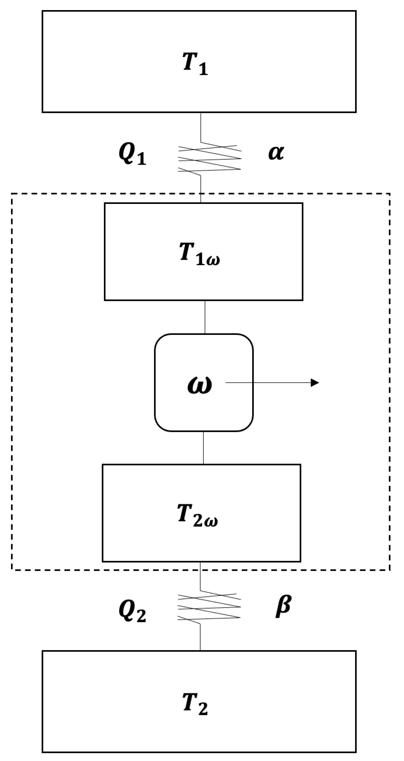
The thermal machine is made up of two temperature stores

T_{1}

and

T_{2}

where

T_{1} > T_{2}

, two irreversible components that are the two thermal resistances, which produce thermal flows towards the reversible Carnot machine with intermediate temperatures

T_{1 w}

and

T_{2 w}

with

T_{1 w} > T_{2 w}

, placed between the intermediate stores. The model considers a linear heat transfer between two irreversible components(thermal conductances

α

and

β

) conductances (see Figure 1.- Scheme proposed by De Vos) [10].

A problem solved by finite-time thermodynamics efficiently is the so-called weak young Sun paradox proposed by Sagan and Mullen [2]. This study presents a drawback for understanding the early stages of planet Earth since the Sun’s luminosity about 4.5 Gyr ago was around 70-80 percent of its value to act [1][2][3]. It represents a terrestrial temperature below the freezing point of water. The planet’s surface temperature is known to be controlled by the solar radiation it receives and its interaction with the gases in the atmosphere. Assuming a blackbody radiative balance between the young Sun and the Earth results in a surface temperature T=255 K, low enough to keep most of the planet’s surface frozen down to 1-2 Gyr [2]. However, several studies, together with sedimentary records, suggest the existence of an average surface temperature capable of having liquid water for almost the entire history of the planet [2]. So, to resolve such a paradox, the first hypothesis is taken that solar radiation has increased in the Sun’s lifetime due to the increase in density of the solar nucleus[2]. The luminosity of the young Sun has been estimated to be 30% less than the present value received from the Sun according to what was said by Gough [2], where

I_{s c}

is the present luminosity of the Sun and

t_{0} \approx 4.56 G y r s

which is the present age of the Sun. The equation (1) shows the evolution of the Sun’s luminosity, and this equation affects the amount of average solar radiation

\bar{q_{s}} = I_{s c} (1 - ρ) / 4

received by the planet. The equation of the luminosity of Gough is expressed in the following way:

I (t) = {[1 + 0.4 (1 - \frac{t}{t_{0}})]}^{- 1} I_{s c}

(1)

Based on foundation, the problem of thermodynamic equilibrium between the solar system’s planets depends on the incident solar influx

I_{s c}

, the planet’s albedo

ρ

, and the greenhouse effect

γ

. Thus, the problem of the thermal balance between planets of the solar system and a correct temperature estimation is solved based on the atmosphere’s physical characteristics. An approach by Finite-Time Thermodynamics (FTT) was raised in work published by Curzon and Ahlborn in 1975 by modeling a Carnot cycle with finite heat transfer between the heat reservoir and the working substance under a maximum power operating regime[4]. Subsequently, the FTT has been developed considering other operating regimes such as efficiency power, ecological function, and others. Models created with the FTT approach provide more realistic real-world power converters operating levels. In 1989, Gordon and Zarmi (GZ) proposed an atmospheric convection model to calculate the temperature of the lowest layer of the Earth’s atmosphere and an upper limit of the average wind power [5]. The GZ model consists of a convection cell, an endoreversible Carnot cycle, and two thermal reservoirs external to the working substance (such as air). De Vos and Flater [6] considered that in the endoreversible model, there is a dissipation of wind energy and obtain an upper limit for the efficiency of conversion of solar energy into wind energy given by

w_{m a x} \approx 8.3 %

assuming the atmospheric "heat engine" is powered by a complete power engine [6]. On the other hand, Van der Wel improved a new efficiency of solar energy upper bound

w_{m a x} \approx 10.23 %

with another model endoreversible based on convective Hadley cells [7][8]. These types of GZ models were used to propose a possible solution to the so-called paradox of the young and weak Sun, which was initially presented by Carl Sagan and George Mullen in 1972 [1] [2,3]. GZ model and the Gough model are applied to the evolution of the solar constant to study the possible future scenarios of Earth’s temperature using different objective functions such as maximum power, efficient power, and ecological function.

Thus, the present work proposes a study of the planet’s surface temperatures due to the increase of greenhouse gases by working to the atmosphere in a thermodynamic regime of finite times. We decided to employ this methodology, considering the good results in predicting climate change in several geologic eras in the past. So, it is possible to modify and set the endoreversible machine model to forecast temperatures derived from climate change in the coming years.

The rest of the manuscript is structured as follows: the next section comprises the literature review on climate change models based on different approaches. Section 3 describes the preliminary foundations concerning Finite-Time Thermodynamics; Section 4 outlines the methods related to the proposed endoreversible model; and Section 5 describes the proposed model and its peculiarities. Section 6 shows the experimental results, and the discussion of the outcomes and findings are included in Section 7, and the last section involves the conclusion and future works.

2. Related work

Global warming caused by human activities represents one of the most significant challenges of the present time. The classical approaches concerning climate change have studied complex systems such as differential equations and developments in chaos theory. Nevertheless, the large amount of data available allows us to use Artificial Intelligence techniques, which are more straightforward than those used by the areas of complexity science, resulting in the prediction of future scenarios due to climate change.

According to Houghton [23], global warming has a climate system where several variables are responsible for raising global average temperatures. Most of these effects are related to the radiative balance of the planetary atmosphere: water vapor feedback, cloud-radiation feedback, and ocean-circulation feedback. In consequence, all of them refer to the albedo and greenhouse effects. Therefore, to forecast global warming, a set of characteristics that affect the global emission of greenhouse gases must be taken. These gases have had a notable increase due to anthropogenic behavior and activity. Development projections of global average temperature changes for the present century are in the range of 0.15C°-0.6C° per decade. Understanding this problem allows us to consider humans’ and ecosystems’ impacts and adaptive capacity [23].

One of the main effects of global warming is the melting of ice bodies on the Earth. The Arctic Sea is one of the leading indicators of the increase in average temperature. The study of the ice concentration and the rise in sea level has various approaches, one of which is widely used is the Deep Learning techniques to predict how the ice concentration changes with the increase in average temperature [24]. In the same way that the arctic layers and their melting show the effect of climate change, all oceans experience the same significant warming and a rising sea level, so it is necessary to generate diagnostic and prognostic prediction models to elucidate these increases and their risks since they are associated with other adverse events such as the propagation of cycles, lack of rain and the growth and spread of diseases. According to diverse authors, the combination of machine learning and deep learning techniques can give us entirely accurate predictions for the future [25,26,27], and [28].

In the study carried out by Balsher Singh Sidhu of the University of British Columbia [18], the use of machine learning is analyzed to understand the impact of climate change on different types of crops, taking into account the climate-yield relationships. The authors compared the usual linear regression (LR) technique for estimating historical data to approximate yield against climate change and using boosted regression trees (BRTs). The conclusions suggest that interpreting results based on a single model can generate biases in the information obtained.

On the other hand, due to the high economic and social impacts associated with climate change, it is essential to understand the causes of this and identify the patterns of the data obtained to make correct predictions. According to Zheng, H. [19], the construction of a reliable model based on experimental data and the relationship between temperature and the concentration of gases in the atmosphere such as carbon dioxide

(C O_{2})

, nitrous oxide

N_{2} O

and methane

(C H_{4})

, is the first challenge to address the climate change problem. Zheng’s study used various learning techniques, such as linear regression, lasso, support vector machines, and random forest, to build an accurate model that would identify changes in the atmosphere increasing temperature dominated mainly by the increase in temperature of

C O_{2}

due to its higher concentration within greenhouse gases.

According to several authors, the construction of a reliable model combined with the temperature data set and machine learning prediction tools will help us to have a better understanding of the phenomenon and thus be able to make a good forecast that allows us to face the risks of climate change. The thermal equilibrium model was studied by De Vos and Flater, among others [8], who analyzed solar radiation as an energy converter used to examine the average temperature of a planet. It is done by the radiation from the planet’s surface and the irradiance reaching Earth. This analysis takes into account the physical characteristics of the atmosphere, such as friendliness and the albedo effect [4,6,8]. Thus, the total flux Q appears as shown in Equation 2.

Q = 4 π R^{2} σ ((1 - ρ) \frac{f}{4} T_{s}^{4} - (1 - γ) T_{p}^{4})

(2)

It is the first thermodynamic model that allows a dynamic study of the different layers of the atmosphere, the lowest layer corresponding to the temperature on the planetary surface. This development can analyze various scenarios where greenhouse gases and albedo concentrations are modified. The feasibility of the model was tested in the study of geological eras, and several authors carried out the solution of the faint young Sun paradox [1,2]. This study of the solar converters under the regime of finite time thermodynamics was analyzed in this work, changing the parameters to current time considering the increase of

C O_{2}

main greenhouse gas [19] its relationship with albedo was developed in this work. In addition, a dissipation of energy in the system is considered to have realistic results at the current time.

3. Preliminary

3.1. The Finite-time Thermodynamics(TTF)

The endoreversible Carnot machine is not in thermodynamic equilibrium with the reservoirs and the active substance. There is a separation between the internally reversible processes and the irreversibilities at the system boundaries, where internal processes with fast relaxation times can be considered reversible and the entropy change for the thermodynamic universe

Δ S_{u}

of the machine is positive, the entropy being of our null working substance

Δ S_{w} = 0

. This definition is known as the endoreversibility hypothesis; when the model proposed by Curzon and Ahlborn[4] evolves in finite time, the model’s power is non-zero, unlike that given by CET [11].

3.2. Curzon and Ahlborn Engine

The engine has thermal conductances that comply with Fourier’s law for heat conduction (

\dot{Q} = - λ \nabla T

). In the present work, we will use the following notation to refer to the heat flows

Q = \dot{Q}

, such that:

Q_{1} = α (T_{1} - T_{1 w})

(3)

Q_{2} = β (T_{2 w} - T_{2})

(4)

A form of solution to the Curzon and Ahlborn[4] engine and the machine schematic was proposed by Alexis De Vos[6]. From the conservation of energy, we have that the heat flow

Q_{1}

from the upper reservoir, towards the reversible machine with power P to the output flow

Q_{2}

[12].By the entropic conservation of the system

Σ S = 0

. Therefore, the production of entropy must be zero, whereas, for the reversible internal machine, we assume that its entropy changes are zero (endoreversibility hypothesis) [8,10,12,13].

σ = \frac{Q_{1}}{T_{1} w} - \frac{Q_{2}}{T_{2} w} = 0

(5)

From equation (5) with the second law of thermodynamics, we have the following relationship for thermal conductors

T_{1 w}

and

T_{2 w}

T_{1 w} = \frac{α}{α + β} T_{1} + \frac{β}{α + β} \frac{1}{1 - η} T_{2}

(6)

T_{2 w} = \frac{α}{α + β} (1 - η) T_{1} + \frac{β}{α + β} T_{2}

(7)

Substituting

T_{1 w}

in equation (3) and

T_{2 w}

in equation (4) with our flow

Q_{1}

and

Q_{2}

, we obtained Equation (3) and Equation (4).

Q_{1} = γ \frac{T_{1} - T_{2} - T_{1} η}{1 - η}

(8)

Q_{2} = T_{2} (\frac{β (T_{1} (1 - η) - T_{2})}{γ (1 - η) T_{1} + β T_{2}})

(9)

with the expression:

γ = \frac{α β}{α + β}

Thus, from the definition of efficiency, we can obtain an expression for the power given by:

P = γ \frac{η (T_{1} - T_{2} - T_{1} η)}{1 - η}

(10)

Resulting in efficiency at maximum power for the Curzon-Ahlborn machine known in finite-time thermodynamics as

η_{c a}

that satisfies

0 < η_{c a} < η_{c}

η_{C A} = 1 - \sqrt{\frac{T_{2}}{T_{1}}}

(11)

In the endoreversible Curzon-Ahlborn model, the dissipation will be given by formulas that have been derived that show the efficiency of an engine under maximum power conditions [5,9].

Φ_{r b} = Q_{2} - \frac{T_{2}}{T_{1}} Q_{1}

(12)

4. Materials and Methods

4.1. Gordon and Zarmi (GZ) model

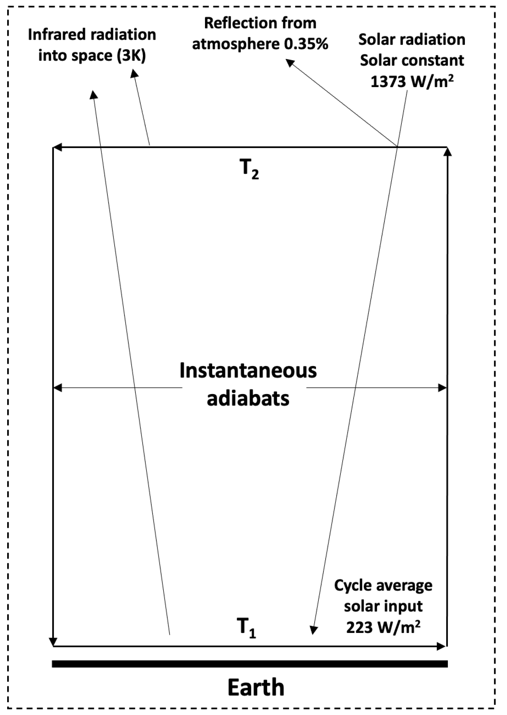
The atmospheric convection model proposed by GZ consists of a cell as an endoreversible Carnot cycle between two thermal reservoirs of extreme temperatures, the temperature

T_{1}

is the working fluid (atmosphere) temperature at the lowest altitude in the system is related with the temperature of Earth’s surface , the temperature in the highest part of working flui is the cold reservoir in the model of GZ, the temperature is related with the cosmic background radiation

T_{2} = 3 K

(see Figure 2) [5]. The input energy is solar radiation, the active substance is the atmosphere, and the work done by the fluid of the thermal machine is the mean power of the winds. The components of the GZ convention cell are two isothermal branches in which the atmosphere receives heat at low altitudes. The other releases heat at high altitudes of the universe and two intermediate adiabatic branches that are taken as instantaneous [14]. GZ maximized the work per cycle W, subject to thermodynamic restrictions and the average solar radiation flux

q_{s}

[5,14].

\bar{q_{s}} = \frac{I_{s c} (1 - ρ)}{4}

(13)

The GZ model works with a Sun-Earth-Wind system as an endoreversible engine, where the input heat is solar radiation, the active substance is the Earth’s atmosphere, and the labor produced by this cycle is the mean power of the winds. The cold store for this machine is outer space with the temperature of the cosmic background radiation of 3K [5]. A schematic view of the simplified system shows its isothermal and adiabatic branches.

Two isothermal branches in the atmosphere absorb solar radiation at low altitudes, and the other in which the atmosphere rejects heat at high altitudes [5].
Two intermediate instantaneous adiabats with ascending and descending air currents [5].

The temperatures of the four-cycle branches are as follows:

T_{1}

is the temperature of the working fluid in the isothermal branch at the lowest altitude where the working fluid absorbs solar radiation every half cycle. During the second half of the cycle, the heat is rejected through blackbody radiation from the working fluid at temperature

T_{2}

(highest cell altitude) to the cold reservoir bear at

T_{e x}

temperature (3K background radiation of the universe) [5,7].

This model maximizes the work per cycle (average power) according to certain thermodynamic restrictions. From the first law of thermodynamics for this model, we have the following:

Δ U = - W + \int_{t = 0}^{t = t_{c}} q_{s} (t) - σ [T^{4} (t) - T_{e} x^{4} (t)] d t = 0

(14)

Where

Δ U

is the change in internal energy of the active substance,

σ

the Stefan-Boltzman constant

(5.67 X 10^{-} 8 \frac{W}{m^{2} K^{4}})

t_{c}

the cycle time and T the temperature of the active substance. The entropy change is subject to the endoreversibility restriction.

Δ S = \int_{t = 0}^{t = t_{c}} (\frac{q_{s} (t) - σ [T^{4} (t) - T_{e x}^{4} (t)]}{T (t)}) d t = 0

(15)

The variables T,

T_{e x t}

are functions associated with the time.

T (t) = \{\begin{matrix} T_{1} 0 \leq t \leq t_{c} / 2 \\ T_{2} t_{c} / 2 \leq t \leq t_{c} \end{matrix}

(16)

T_{e x} (t) = 3 k 0 \leq t \leq t_{c}

(17)

The variable

q_{s}

is a function of time,

I_{s c}

is the average solar constant over the Earth’s surface

(1372.7 W / m^{2})

, the average albedo

ρ = 0.35

, and the average values are the follows:

q_{s} (t) = \{\begin{matrix} I_{s c} (1 - ρ) / 2 0 \leq t \leq t_{c} / 2 \\ 0 t_{c} / 2 \leq t \leq t_{c} \end{matrix}

(18)

\bar{T} = (T_{1} + T_{2}) / 2

(19)

\bar{T^{n}} = (T_{1}^{n} + T_{2}^{n}) / 2

(20)

The mean power of the winds is obtained by:

P = \frac{W}{t_{0}} = \bar{q_{s} + σ T_{e x}^{4}} - σ \bar{T^{4}}

(21)

The model used by GZ considers the following approximation

\bar{q_{s}} > > σ T_{e x}^{4}

we have the following Equation:

P = \bar{q_{s}} - σ \bar{T^{4}}

(22)

From the endoreversibility condition, the variables T,

T_{e x}

and the mean values we obtained:

Δ S_{i n t} = \frac{\bar{q_{s}}}{T_{1}} - \frac{σ}{2} (T_{1}^{3} + T_{2}^{3})

(23)

To maximize P subject to the endoreversibility condition, the Lagrangian is defined in terms of the Lagrange multiplier

λ

and the thermodynamic constraint given by

L = P - λ Δ S

so that:

L = T^{4} (t) + λ [q_{s} (t) / T (t) - σ T^{3} (t)]

(24)

Finding the extreme of L, that is, solving

\frac{\partial L (t)}{\partial T (t)} = 0

for which we have the following system of equations:

T_{1}^{5} (t) + 3 σ λ T_{1}^{4} / 4 - λ q_{s} (t) / 4 = 0

(25)

T_{2}^{5} (t) + 3 σ λ T_{2}^{4} / 4 = 0

(26)

GZ found the following temperature values for the lowest and highest layers of the Earth’s atmosphere

T_{1} = 277 K

T_{2} = 192 K

and

P_{m a x} = 17.1 \frac{W}{m^{2}}

. These values are not far from the literature

P_{m a x} = 7 \frac{W}{m^{2}}

T_{1} = 290 K

(on the surface) and

T_{2} = 195 K

(between 75 and 90km). Gordon and Zarmi[5] stated that their mean power of winds should be taken as an upper limit.

4.2. Nonendoreversibility parameter in G-Z

In recent studies, the nonendorevesibility parameter R has been used to investigate the thermal machines of TTF. This parameter was introduced from the Clausius inequality, considered a clearance measure in the endoreversible regime [15].

Δ S_{w 1} + Δ S_{w 2} \leq 0

(27)

Δ S_{w 1}

change in the hot isotherm and

Δ S_{w 2}

in the cold compression isotherm, in the endoreversible case. Thus, this inequality becomes equality in the following equation.

Δ S_{w 1} + R Δ S_{w 2} = 0,

(28)

where R is given by:

R = \frac{Δ S_{w 1}}{∥ Δ S_{w 2} ∥}

(29)

Where

R = \frac{Δ S_{w 1}}{∥ Δ S_{w 2} ∥}

parameter of non-endoreversibility is in the interval

0 \leq R \leq 1

, where R=1 is the endoreversible limit [12]. The previous GZ convection cell process is enriched using the parameter R. Thus, to maximize P subject to the endorreversibility condition plus the parameter R, the Lagrangean

L = P - λ Δ S

to occupy is given as follows:

L = \frac{σ}{2} (T_{1}^{4} + T_{2}^{4}) + λ [\frac{\bar{q_{s}}}{T_{1}} - \frac{R σ (T_{1}^{3} + T_{2}^{3})}{2}]

(30)

Solve

\frac{\partial L (t)}{\partial T (t)} = 0

to find the extrema of the Lagrangian, solving the system numerically, it is found that for a nonendoreversibility parameter R=0.953 [15] for

ρ = 0.35

I_{s c} = 1372.7 W / m^{2}

GZ found the following temperature values for the lowest and highest layers of the Earth’s atmosphere

T_{1} = 280.562 K

T_{2} = 194.293 K

5. The proposed model

5.1. Greenhouse factor

The planet’s surface temperature calculations are modified by adding the greenhouse parameter

γ

. Therefore, it is necessary to add the greenhouse effect to the equations proposed by the thermodynamics of finite times, to obtain the temperatures of the lower and upper layers of our active substance (air). Thus, the equations for entropy and internal energy are also changed.

Δ U = - w + \int_{t = 0}^{t = t_{c}} q_{s} (t) - σ (1 - γ) [T^{4} (t) - T_{e} x^{4} (t)] d t = 0

(31)

Equation (15) is expressed in terms of the nonendoreversibility parameter and the greenhouse factor, giving as a result the following expression:

Δ S = \int_{t = 0}^{t = t_{c}} (\frac{q_{s} (t) - R (1 - γ) σ [T^{4} (t) - T_{e x}^{4} (t)]}{T (t)}) d t = 0

(32)

From the G-Z section the average power of the winds

P = \frac{w_{c}}{t}

in which

\bar{q_{s}} > > σ T_{e x}^{4}

the power expression output for the case of greenhouse effect is of the form:

P = \bar{q_{s}} - \frac{σ}{2} (1 - γ) [T_{1}^{4} + T_{2}^{4}]

(33)

Equations (31) (32) show us a greenhouse factor acting on the two layers of the atmosphere with temperatures

T_{1}

and

T_{2}

. To maximize P subject to the endoreversibility condition, we defined the Lagrangian in terms of the Lagrange multiplier

λ

and the thermodynamic constraint given by

L = P - λ Δ S

so that:

L = \bar{q_{s}} - \frac{σ}{2} (1 - γ) [T_{1}^{4} + T_{2}^{4}] - λ \{\frac{{\bar{q}}_{s}}{T_{1}} - \frac{σ}{2} (1 - γ) [T_{1}^{3} + T_{2}^{3}]\}

(34)

Where

λ

is a Lagrange multiplier by solving the Euler-Lagrange equations

\frac{\partial L (t)}{\partial T (t)} = 0

, a system of equations is obtained, which allows us to calculate the extremes of the power.

For

\frac{\partial L (t)}{\partial T_{1} (t)} = 0

T_{1}^{5} - \frac{3}{4} R λ T_{1}^{4} - \frac{\bar{q_{s}}}{2 σ (1 - γ)} = 0

(35)

For the case

\frac{\partial L (t)}{\partial T_{2} (t)} = 0

T_{2} = \frac{3 R}{4} λ

(36)

Finally for

\frac{\partial L (t)}{\partial λ} = 0

we have:

\frac{{\bar{q}}_{s}}{T_{1}} - \frac{σ}{2} (1 - γ) [T_{1}^{3} + T_{2}^{3}] = 0

(37)

Eliminating

λ

and giving the value of

q_{s} \approx 229 W / m^{2}

[11], we have two equations whose numerical solution provides the highest and lowest layer surface temperatures. The low of the Earth’s atmosphere under a regime of maximum power in terms of the non-endo reversibility parameter R, the albedo

ρ

, the greenhouse effect

γ

, and the current solar constant

I_{s} c

T_{1}^{5} - T_{2} T_{1}^{4} - \frac{2 q_{s}}{3 R σ (1 - γ)} T_{2} = 0

(38)

T_{1}^{4} + T_{2}^{3} T_{1} - \frac{2 \bar{q_{s}}}{R σ (1 - γ)} = 0

(39)

5.2. Greenhouse factor in the lowest layer of the atmosphere average surface temperature

The power for the G-Z model is given by

P = \frac{w_{c}}{t}

, where for

T_{e x} = 3 K

\bar{q_{s}} > > σ T_{e x}^{4}

the output power expression with greenhouse effect in the lower part is the following:

P = \bar{q_{s}} - \frac{σ R}{2} [(1 - γ) T_{1}^{4} + T_{2}^{4}]

(40)

It is necessary to maximize P subject to the endoreversibility condition and the greenhouse effect at the bottom, so the Lagrangian is defined in terms of the Lagrange multiplier

λ

and the constraint on thermodynamics showing the following Lagrangian expression:

L = \bar{q_{s}} - \frac{σ}{2} [(1 - γ) T_{1}^{4} + T_{2}^{4}] - λ \{\frac{{\bar{q}}_{s}}{T_{1}} - \frac{σ}{2} [(1 - γ) T_{1}^{3} + T_{2}^{3}]\}

(41)

Solving the Euler-Lagrange equations

\frac{\partial L (t)}{\partial T (t)} = 0

, we obtain the following equations:

For

\frac{\partial L (t)}{\partial T_{1} (t)} = 0

T_{1}^{5} - \frac{3}{4} R λ T_{1}^{4} - \frac{\bar{q_{s}}}{2 σ (1 - γ)} = 0

(42)

For

\frac{\partial L (t)}{\partial T_{2} (t)} = 0

T_{2} = \frac{3 R}{4} λ

(43)

For

\frac{\partial L (t)}{\partial λ} = 0

we have:

\frac{{\bar{q}}_{s}}{T_{1}} - \frac{σ}{2} [(1 - γ) T_{1}^{3} + T_{2}^{3}] = 0

(44)

From (42),(43),(44) removing the parameter

λ

, we obtain:

T_{1}^{5} - T_{2} T_{1}^{4} - \frac{2 \bar{q_{s}}}{3 R σ (1 - γ)} T_{2} = 0

(45)

T_{1}^{4} + \frac{1}{(1 - γ)} T_{2}^{3} T_{1} - \frac{\bar{2} q_{s}}{R σ (1 - γ)} = 0

(46)

The models proposed by De Vos, Gordon, and Zarmi[6][5] can compute the temperatures of the atmosphere of some past or future periods of the Earth, as was done in the study by Angulo and Barranco-Jiménez [2], where the temperatures of early age are calculated with enough accuracy. In the present work, we worked similarly, but for a future time of the atmosphere (prediction event), we considered the atmosphere’s physical characteristics, such as the albedo greenhouse effect. The model created by De Vos shows an excellent relationship between the theoretical and experimental data. Our proposed work approximated the albedo dependent on the greenhouse effect with a=0.072, b=0.4955, and c=0.1527.

ρ = a γ^{2} + b γ + c

(47)

The GZ-type models with the greenhouse factor and the albedo condition above, and the atmosphere represented by the equations 45 and 46, allow us to obtain temperatures of the highest and lowest layer of the atmosphere. It is necessary to determine the atmospheric characteristics of the GZ-type models. According to the solution of the faint young Sun paradox presented by Angulo and Barranco [2], the finite-time thermodynamics models efficiently resolve the paradox, calculating the planet’s average surface temperature from different geological stages. Using scenarios where the luminosity of the Sun is taken into account through the Gough 1 equation, it is necessary to modify this equation to actual luminosity as represented in the following equation.

I (t) = {[1 + 0.4 (1 - \frac{t + t_{0}}{t_{0}})]}^{- 1} I_{s c}

(48)

Using the albedo

ρ

, the average solar radiation flux, and greenhouse coefficient

γ

, we modified the scheme proposed by Angulo and Barranco to determine the effects of climate change due to the increase in greenhouse gas, taking the relationship proposed in our work. That relationship between the albedo and greenhouse effect is represented in equation 47, including the present-day values for average luminosity, its variation per year (equation 48), and the changes directly proportional to the flux

q_{s}

expressed in 13. Nevertheless, it is necessary to consider the dissipation in the maximum power regime to obtain realistic results. This modification allows obtaining results to predict the effects of climate change in future years. Thus, the average temperature of the surface (

T_{s}

) at present will be based on the existing relationship in the dissipation 12 of the system in maximum power conditions in the GZ-type model equations 45 and 46.

T_{s} = T_{1} + T_{2} (\frac{β (T_{1} (1 - η_{C A}) - T_{2})}{γ (1 - η_{C A}) T_{1} + β T_{2}}) - \frac{T_{2} γ (T_{1} - T_{2} - T_{1} η_{C A})}{T_{1} (1 - η_{C A})}

(49)

Simplifying:

T_{s} = T_{1} + T 2 (\frac{T 1 (1 - η_{C A}) - T 2}{(1 - η_{C A}) T 1 + T 2}) - \frac{T_{2}}{T_{1}} (\frac{(T 1 - T 2 - T 1 η_{C A})}{(1 - η_{C A})})

(50)

6. Experimental Results

It is necessary to determine possible and future scenarios for the growth of greenhouse gases. Most of the concentration of gases in the atmosphere has presented a significant increase since the 70s due to industrial activities. According to Mauna Loa laboratory in Hawaii [14] [29], data shows a massive rise in

C O_{2}

by the empirical formula concentration for the interval

1975 \leq t \leq 2100

[14]. So, the expression obtained by Wubbles concerning the trace gas trends and their potential role in climate change is valid for this methodology [14].

[C O_{2}] = 330^{e^{0.0056 (t - 1975)}}

(51)

According to equation 47, the albedo and the greenhouse effect are related. For the Earth, the value of the greenhouse effect can be defined as

γ = (E_{s} - F) / E_{s}

, where

E_{s}

is the surface emission, and F is the outgoing radiation [2]. Moreover, it is noticed that the increase in greenhouse gases rises over time, according to Wubbles and different experimental measurements. With all these characteristics, the natural average temperature (

T_{s}

) and its possible evolution in the coming years can be determined with reasonable accuracy.To test the GZ model that considers a dissipation

ϕ_{r b}

developed in this work, solving numerically with

R = 1

and different values of

γ

and

ρ

related to the year. It is a data compilation by Berkeley Earth. The study shows the temperature of the Earth’s surface, and the experimentally measured temperatures

T_{o b s}

were compared against our theoretically calculated temperatures

T_{s}

to use a forecasting technique later to determine the future of temperatures.

6.1. Data pre-processing

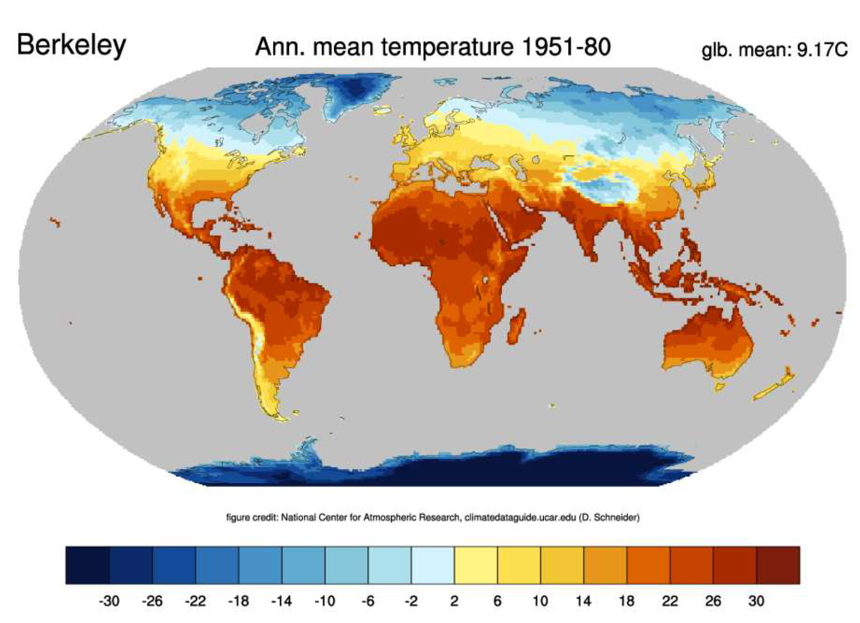
To analyze the complexity of climate change, the terrestrial and oceanic temperatures of the planet are measured. The used data is a compilation of data provided by Berkeley Laboratory. Other widely used datasets are MLOST NOAA Land-Ocean Surface Temperature and GISTEM from NASA [20][21][22]. The data compilation by Berkeley records Land Average temperatures in the format yyyy/mm/dd. So, a split was made by year, month, and day taking the temperature of each month, and the mean temperature per year was computed. It is observed that there is a correlation with a value of 0.89 between the variables of the year and the Land Average Temperature from the year 1975 to 2015 [20][21][22]. Figure 3 shows the climatology of the average annual terrestrial temperature between 1951 and 1980 from the Berkeley Earth Data with a global mean of 9.17 Celsius. In our work, the mean experimental temperature of each year is compared with that obtained in the theoretical model developed.

The results of the data and the surface temperatures

T_{s}

obtained from the model expressed in the equation 50 that was developed in this work are shown in Table 1. All the results regarding data are presented in Celsius degrees.

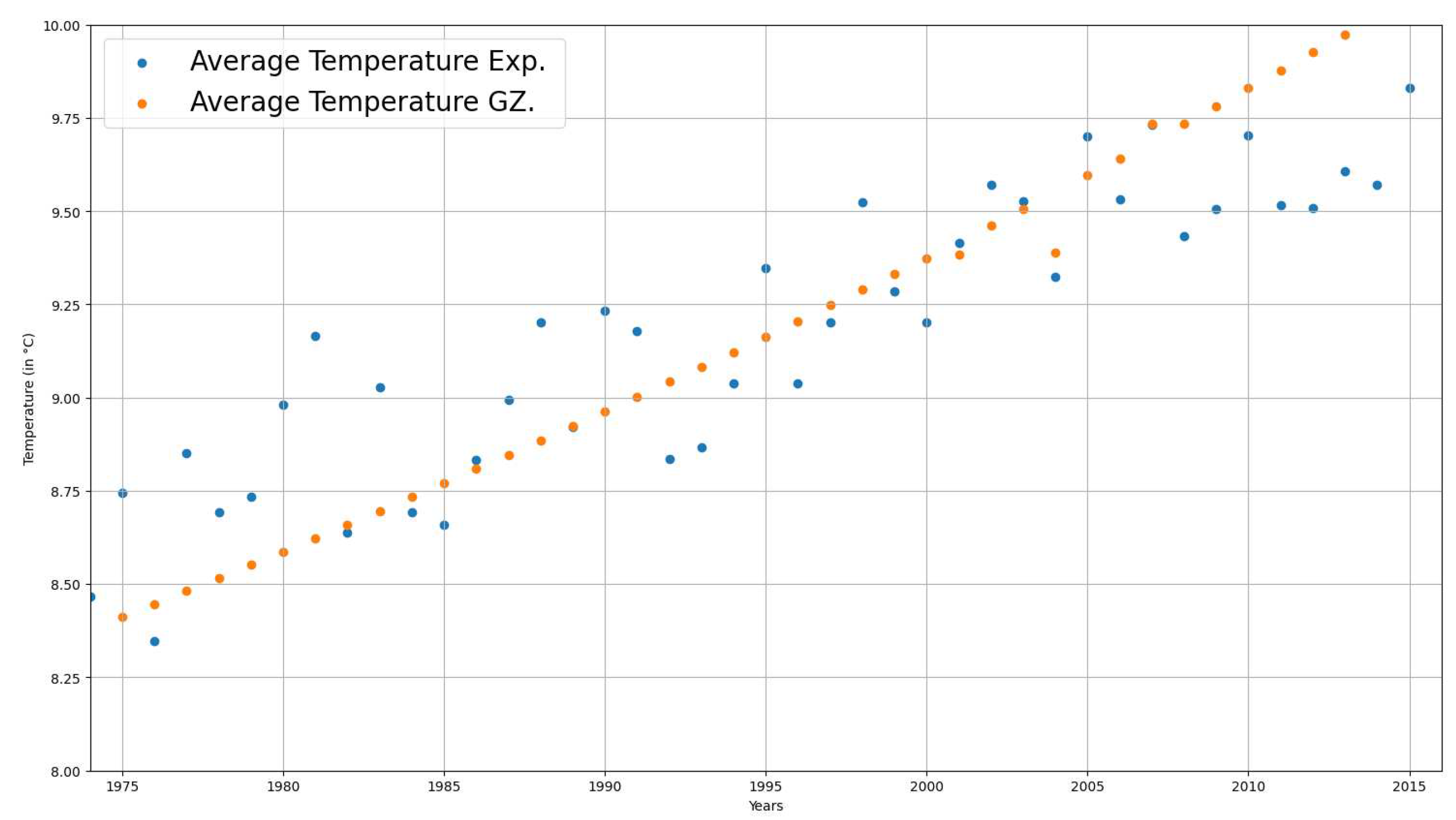
The temperature increase due to greenhouse gas growth has been analyzed since 1975. It was fixed this year because of the significant increase in the concentration of

C O_{2}

as shown by the experimental development of Wubbles in equation 51; when seeing the correlations of the observational variables of the temperature of the Berkeley database. We can notice a high correlation between the year and the land’s Average Temperature, and the correlation is equal to 0.89. Therefore, a linear regression model is sufficient in this case to make a future prediction of the temperature. In the following plot (Figure 4. Average temperatures observed and calculated by the GZ-type model), we can observe a relationship between the average temperature per year measured against the temperature of the modified GZ model.

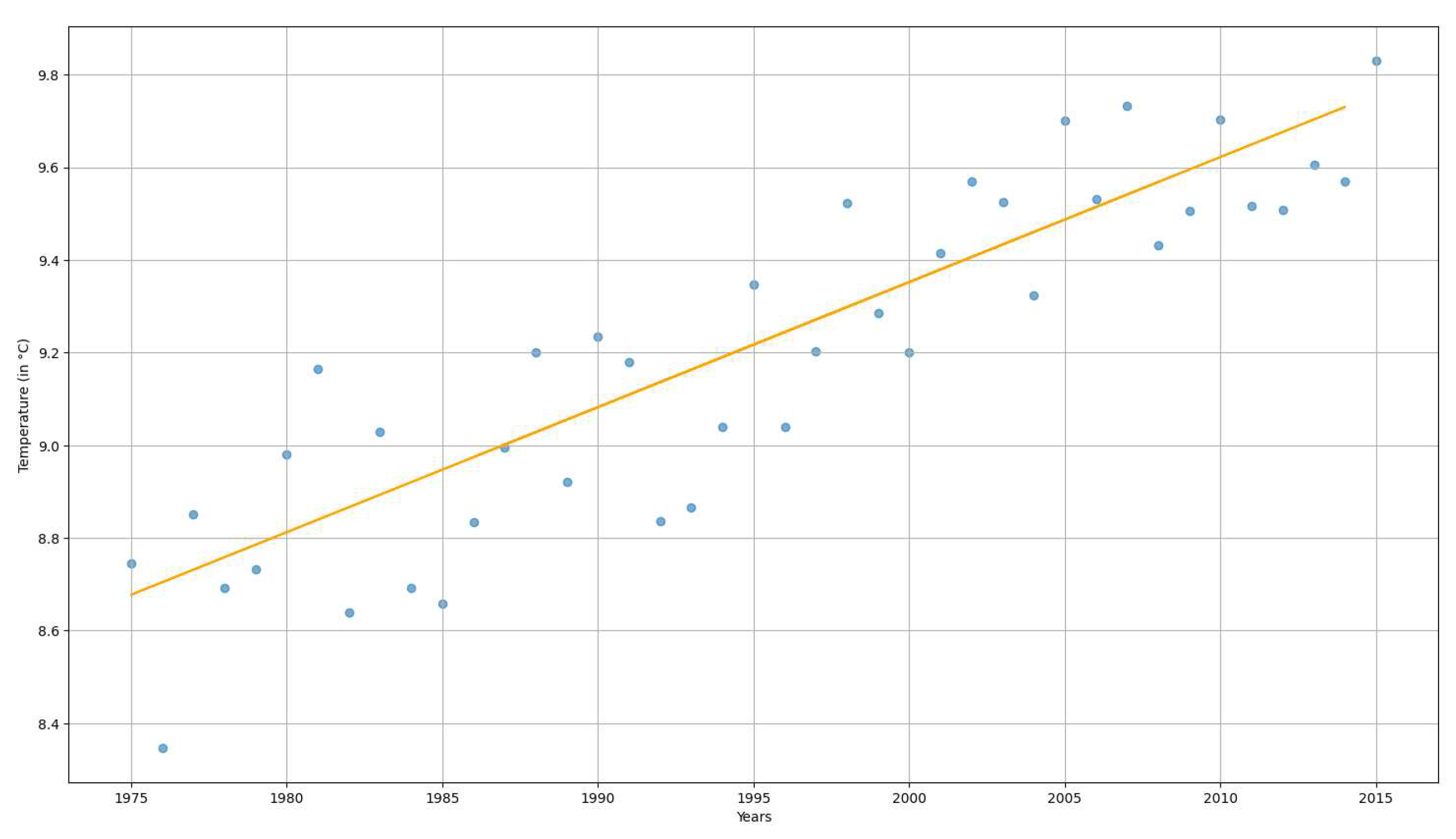
Thus, (Figure 5. Average temperatures observed since 1975 with linear regression.) shows how a linear regression adjusts perfectly to predict the evolution of the temperature from the year 1975. It is possible to infer how the temperature change will be towards the year 2100 thanks to this type of modeling.

On the other hand, Table 2 presents the future prediction of the temperatures using linear regression (LR), Ridge Regression (RR), and Artificial Neural Networks (ANN). Thus, the ANN has five layers: an input layer with a linear activation function, three layers with a e rectified linear activation function or Relu or ReLU for short, and an output layer with a linear activation function. All techniques were applied to the observed temperatures (

T_{o b s}

) and the models’ temperatures used in the present work. In the same way, the third column shows the temperatures calculated (

T_{s}

) from our model of Gordon and Zarmi (GZM) without applying a linear regression, where the physical characteristics of the atmosphere are taken into account and what theoretical temperature would be reached. In addition, Table 2 depicts the entire prediction made up to 2100, starting in 2016.

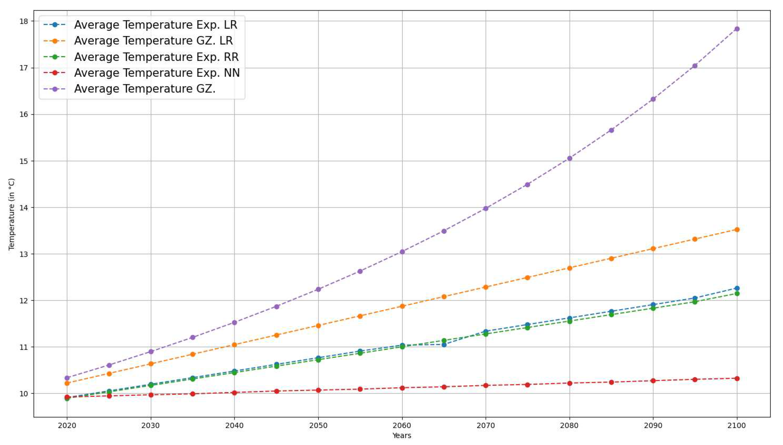
Moreover, Figure 6 shows the evolution of the surface temperature (

T_{s}

), according to the predictions made by the model proposed in our work with the initials GZM and the temperature prediction from the experimental data (

T_{o b s}

). Thus,

T_{S}

and

T_{o b s}

were forecasted using machine learning techniques.

From a correlation analysis between the temperature variables under different machine learning techniques such as Linear Regression (LR), Ridge Regression (RR), Artificial Neural Networks (ANN), and the proposed endoreversible model (GZM), it can be observed that the GZM model is more suitable with a linear relationship (see Figure 7).

7. Discussion

In this analysis of climate change, an endoreversible modeling of the Gordon and Zarmi type was carried out. Unlike other finite-time thermodynamic studies for studying the atmosphere, adjustments were made to give the model realistic results if applied. As for the climatic analysis of geological eras, as observed in other works, it is noticed that the results do not correspond to what is reported by observations of the current temperature. According to Levario, Valencia, and Arias [9], for a correct thermodynamic optimization of power plants, it is necessary to consider the system’s variations. Therefore, the modeling was performed considering those variations, the change in luminosity per year, the increase in greenhouse gas, and its relationship with the terrestrial albedo, thus adapting it to our model of winds at maximum power. In this way, the family of equations 45 to the equation 51 complement the system to calculate climate change due to atmospheric conditions and the increase in greenhouse gases by anthropogenic conditions.

From Table 1, an increase in the average temperature of the Earth’s surface can be seen from 1975 to 2015, both in the observational (experimental) model and the theoretical model developed in our work. The rise in temperature in both cases is related to the increase in greenhouse gases in the atmosphere.

In Figure 2, we can appreciate the differences between the points obtained experimentally (observation and measurements in the laboratory) and the modeling proposed in our work. Suppose we observe Figure 3 and correlation analysis. In that case, the experimental points in blue show a high linear tendency, so linear or ridge regression is an excellent technique for correctly predicting temperature increases.

On the other hand, the points of our previously mentioned modeling of the GZM would seem to show the same linear trend, so in Table 2, two comparisons were made taking into account a linear regression $T_{s}$ with LR and an analysis obtained directly from our modeling $T_{s}$ with GZM. As a result, we got a difference between the analysis with LR and GZM. This is explained considering that the temperature observations only recorded points in our vector. In contrast, the modeling records these points, and the physical information of the atmosphere is saved, as well as the thermodynamic variables of the system, which gives us results of mean temperature increase with more value than those obtained by an analysis of experimental points.

Moreover, Figure 3 shows a plot of the predictions made from the experimental data

T_{o b s}

and the modeling of the GZM system. It is important to note that in future scenarios with forecasting by GZM, the average temperature is higher than that obtained by the data of the evolution of the observed temperatures

T_{o b s}

from various machine learning techniques. Nevertheless, the rate of temperature increase is in the range per decade according to [23]. The plot shows that the temperature evolution in the case of the construction of an ANN, LR, and RR grows in a widespread gradual way compared with our proposed model. GZM modeling saves the atmosphere’s physical characteristics, such as entropic relationships, radiation conditions, and irradiance. It helps to present more realistic behavior in the data, unlike the other forecasting that only shows us a regression of the linear type without considering the evolution of the physical parameters caused by the alterations in the Earth’s atmosphere.

8. Conclusion and Future Work

In this article, we proposed a new finite-time thermodynamics approach to predict changes in surface temperature in the lowest layer of the atmosphere that corresponds to the average temperature. The proposed approach considers the evolution in albedo and greenhouse gases, the change in luminosity per year, and the system’s dissipation in the regime of maximum power conditions.

Thus, the increase in temperature is linked to physical conditions such as irradiance and radiation. Moreover, a comparison with different machine learning techniques showed a rise in temperature in all these methods. Nevertheless, machine learning algorithms do not preserve atmospheric information in the period studied; therefore, the forecasting could present a bias in the prediction because these are trained only with experimental data without considering the variables that generate climate change. All the techniques and our modeling demonstrated an increase in temperature. We can conclude the success of our model by comparing it with our experimental data. In addition, according to Houghton[23], the projections of global average temperature changes are in the range of 0.15 °C - 0.6 °C per decade, which is in the field of the values obtained.

Our future works are oriented towards developing other thermodynamic models, such as ecological and efficiency power regimes, assessing these models with approaches based on machine learning. The present proposal studies the atmosphere, considering a wind engine the most common control in obtaining the maximum power as it works. In this paper, studying other regimes will allow us to analyze the whole spectrum of our modeling (wind engine) and thus observe all cases of global warming. All theoretical predictions always will be compared against experimental data to face climate change in the best way.

Author Contributions

Conceptualization, S.V.-R. and M.T.-R.; methodology, R.Q.; software, C.G.S.-M. and K.T.C.; validation, S.V.-R. and M.T.-R.; formal analysis, R.Q. and S.V.-R.; investigation, M.T.-R.; resources, K.T.C.; data curation, C.G.S.-M; writing—original draft preparation, S.V.-R.; writing—review and editing, M.T.-R.; visualization, K.T.C.; supervision, M.T.-R.; project administration, C.G.S.-M.; funding acquisition, K.T.C. All authors have read and agreed to the published version of the manuscript.

Funding

This work was partially sponsored by the Instituto Politécnico Nacional and the Consejo Nacional de Ciencia y Tecnología under grants 20230655, 2023XXXX, and SECTEI-2023, respectively.

Institutional Review Board Statement

Not applicable.

Informed Consent Statement

Not applicable.

Data Availability Statement

Not applicable.

Acknowledgments

We are thankful to the reviewers for their time and their invaluable and constructive feedback that helped improve the quality of the paper.

Conflicts of Interest

The authors declare no conflict of interest.

References

Sagan, C., & Mullen, G.; Earth and Mars: Evolution of atmospheres and surface temperatures. Science 1972, 177.
Angulo-Brown, F., Rosales, M.A. & Barranco-Jimenez, M.A.; The faint young Sun paradox: a simplified thermodynamic approach. Advances in Astronomy 2012, 2012.
Kasting, J.F. & Grindspoon, D.II.; The faint young Sun problem in The Sun in Time. The university of Arizona, Tucson, Ariz, USA 1991, 447–462.
Curzon, F.L. & Ahlborn B.; Efficiency of a Carnot engine at maximum power output. am. J. Phys, 1975, 43, 22–24. [Google Scholar] [CrossRef]
Gordon M. & Zarmi; Wind energy as a solar-driven heat engine: a thermodynamic approach. American Journal of Physics 1989, 57, 995–998. [CrossRef]
De Vos, A., & Flater G. The maximum efficiency of the conversion of solar energy into wind energy. American Journal of Physics 1991, 59, 751–754. [CrossRef]
M.A. Barranco Jiménez and F. Angulos-Brown.A simple model on the influence of the greenhouse effect on efficiency of solar-to-wind energy conversion. Il nuovo Cimento 2003, 26.
A de. Vos & P. van der Wel The effieciency of the conversion of solar energy into Wind energy by mean of Hadley Cells. Theor. Appl. Climatol 1993, 46, 193–202. [CrossRef]
Levario-Medina, S., Valencia-Ortega, G., & Arias-Hernández L. A. , Optimización termodinámica de algunas plantas generadoras de energía mediante la k-Potencia Eficiente.
L.A. Arias-Hernández & F. Angulos-Brown. A general property of endoreversible thermal engines. J. Phys. 1997, 81, 22. [CrossRef]
M.A. Barranco-Jiménez, J.C. Chimal-Eguía & F.Angulo-Brown. (2006) The Gordon and Zarmi model for convective atmosferic cell under the ecological criterion applied to the planets of solar system, Revista mexicana de física 52(3) 205-212 (2006).
Garcia Ocampo Armando, Optimizacion termoeconómica de un modelo de máquina química endorreversible. Instituto Politecnico Nacional 2015.
F.Angulo-Brown., L.A. Arias-Hernández & Santillan M., On some connection between first order irreversible thermodynamics and finite-time thermodynamics. Revista Mexicana de fisica 2002, 48, 182–192.
Norma Sanchez, F.Angulo-Brown & M.A. Barranco-Jiménez. Posibles futuros escenarios de la temperatura superficial de la Tierra con la evolución de la constante solar XXII Congreso Nacional de Termodinámica 2007.
M.A. Barranco Jiménez and F. Angulos-Brown. A nonendereversible model for wind energy as a solar-driven heat engine. J. Appl. Phys. 1996, 80, 22. [CrossRef]
J.A. Curry and P.J. Western. Thermodynamics of Atmospheres & Oceans. International Geophysics Series: Academic Press. 1999.
Angulo-Brown, F., Sanchez-Salas, N., Barranco Jiménez, M.A. & Rosales, M.A. ,Possible future scenarios for atmospheric concentration of greenhouse gases:A simplifies thermodynamic approach. IRenewable Energy 2009, 34, 2344–2352. [CrossRef]
Sidhu, B. S., Mehrabi, Z., Ramankutty, N., & Kandlikar, M.,How can machine learning help in understanding the impact of climate change on crop yields? Environmental Research Letters 2023.
Zheng, H. Zheng, H. ,Analysis of global warming using machine Learning. Computational Water, Energy and enviromental Engineering 2018, 7, 127. [Google Scholar] [CrossRef]
https://berkeleyearth.org/data/.
https://climatedataguide.ucar.edu/climate-data/global-surface-temperatures-best-berkeley-earth-surface-temperatures.
https://data.giss.nasa.gov/gistemp/.
Houghton, J. Global warming. Reports on progress in physics 2005, 68(6), 1343. [Google Scholar] [CrossRef]
Wang, R., Li, L., Gentine, P., Zhang, Y., Chen, J., Chen, X., ... & Lü, G. Recent increase in the observation-derived land evapotranspiration due to global warming. Environmental Research Letters 2020, 17, 024020. [CrossRef]
Chi, J., & Kim, H. C., Prediction of arctic sea ice concentration using a fully data driven deep neural network. Remote Sensing 2017, 9(12), 1305. [CrossRef]
Casthana, T., Krim, H., Sun, X., Roheda, S., & Xie, L., Atlantic hurricane activity prediction: a machine learning approach. Atmosphere 2021, 12(4), 455. [CrossRef]
Nieves, V., Radin, C., & Camps-Valls, G, Predicting regional coastal sea level changes with machine learning. Scientific Reports 2021, 11(1), 1–6.
Khasnis, A. A., & Nettleman, M. D., Global warming and infectious disease. Archives of medical research 2005, 36, 689–696.
Mauna Loa Observatory, Hawaii. https://esrl.noaa.gov/gmd/ccgg/trends/.

Figure 1. Scheme proposed by De Vos [10]

Figure 2. Simplified diagram of a thermal engine driven by solar energy proposed by [5].

Figure 3. Climatology of annual mean land temperature. NCAR, Climate Data Guide [21].

Figure 4. Average temperatures observed and calculated by the GZ-type model.

Figure 5. Average temperatures observed since 1975 with linear regression.

Figure 6. Comparison of the evolution of temperature from the year 2020 to 2100 through theoretical and experimental models.

Figure 7. Comparison of the correlation between year variables and observed temperatures with the theoretical model.

Table 1. Average temperatures observed and calculated by the GZ-type model.

Year	$T_{o b s}$	$T_{s}$
1975	8.74	8.41
1976	8.34	8.44
1977	8.85	8.48
1978	8.69	8.51
1979	8.73	8.55
1980	8.98	8.58
1981	9.16	8.62
1982	8.63	8.65
1983	9.02	8.69
1984	8.65	8.73
1985	8.65	8.77
1986	8.83	8.80
1987	8.99	8.84
1988	9.20	8.88
1989	8.922	8.92
1990	9.23	8.96
1991	9.17	9.00
1992	8.83	9.04
1993	8.86	9.08
1994	9.03	9.12
1995	9.34	9.16
1996	9.03	9.21
1997	9.20	9.24
1998	9.52	9.29
1999	9.28	9.33
2000	9.20	9.37
2001	9.41	9.38
2002	9.57	9.46
2003	9.52	9.50
2004	9.32	9.48
2005	9.70	9.59
2006	9.53	9.64
2007	9.73	9.73
2008	9.43	9.74
2009	9.50	9.78
2010	9.703	9.82
2011	9.51	9.87
2012	9.507	9.92
2013	9.606	9.97
2014	9.570	10.02
2015	9.831	10.07

Table 2. Average temperatures observed and calculated by the GZ type model.

Year	$T_{o b s}$ with LR	$T_{s}$ with LR	$T_{o b s}$ with RR	$T_{o b s}$ with NN	$T_{s}$ with GZM
2016	9.839	10.049	9.845	10.089	10.121
2017	9.842	10.094	9.860	10.094	10.176
2018	9.845	10.135	9.869	10.099	10.228
2019	9.860	10.178	9.884	10.105	10.281
2020	9.885	10.219	9.907	10.110	10.334
2021	9.913	10.251	9.937	10.115	10.387
2022	9.941	10.292	9.967	10.120	10.440
2023	9.969	10.333	9.996	10.125	10.495
2024	9.997	10.374	10.026	10.130	10.550
2025	10.025	10.426	10.056	10.135	10.606
2026	10.053	10.456	10.086	10.140	10.663
2027	10.081	10.497	10.116	10.144	10.720
2028	10.109	10.538	10.146	10.149	10.777
2029	10.137	10.579	10.175	10.154	10.836
2030	10.165	10.620	10.205	10.159	10.895
2031	10.193	10.661	10.235	10.164	10.954
2032	10.221	10.702	10.265	10.169	11.014
2033	10.249	10.743	10.295	10.174	11.018
2034	10.277	10.784	10.325	10.179	11.138
2035	10.305	10.825	10.354	10.184	11.200
2036	10.333	10.866	10.384	10.189	11.263
2037	10.361	10.907	10.414	10.194	11.327
2038	10.389	10.948	10.444	10.199	11.392
2039	10.417	10.989	10.474	10.204	11.456
2040	10.445	11.030	10.504	10.209	11.524
2041	10.473	11.071	10.533	10.213	11.591
2042	10.501	11.112	10.563	10.218	11.659
2043	10.529	11.153	10.593	10.223	11.728
2044	10.557	11.194	10.623	10.233	11.798
2045	10.585	11.235	10.653	10.238	11.868
2046	10.613	11.276	10.683	10.243	11.939
2047	10.641	11.317	10.713	10.246	12.012
2048	10.669	11.358	10.742	10.248	12.085
2049	10.697	11.399	10.772	10.253	12.159
2050	10.725	11.440	10.802	10.258	12.234
2051	10.753	11.481	10.832	10.263	12.311
2052	10.781	11.522	10.862	10.268	12.388
2053	10.809	11.563	10.892	10.272	12.465
2054	10.837	11.604	10.921	10.277	12.545
2055	10.865	11.645	10.951	10.282	12.625
2056	10.893	11.686	10.981	10.287	12.707
2057	10.921	11.727	11.011	10.292	12.789
2058	10.949	11.768	11.041	10.297	12.872
2059	10.977	11.809	11.071	10.302	12.957
2060	11.005	11.850	11.100	10.307	13.043
2061	11.033	11.891	11.130	10.312	13.129
2062	11.061	11.932	11.160	10.317	13.218
2063	11.089	11.973	11.190	10.322	13.308
2064	11.117	12.014	11.220	10.327	13.398
2065	11.145	12.055	11.250	10.332	13.490
2066	11.173	12.096	11.279	10.336	13.584
2067	11.201	12.137	11.309	10.341	13.659
2068	11.229	12.178	11.339	10.346	13.775
2069	11.257	12.219	11.369	10.351	13.872
2070	11.285	12.260	11.399	10.356	13.972
2071	11.313	12.301	11.429	10.361	14.072
2072	11.341	12.342	11.458	10.366	14.174
2073	11.369	12.383	11.488	10.371	14.277
2074	11.397	12.424	11.518	10.376	14.383
2075	11.425	12.465	11.548	10.381	14.490
2076	11.453	12.506	11.578	10.386	14.599
2077	11.481	12.547	11.608	10.390	14.709
2078	11.509	12.588	11.637	10.396	14.820
2079	11.537	12.629	11.667	10.401	14.935
2080	11.565	12.670	11.697	10.405	15.050
2081	11.593	12.711	11.727	10.410	15.168
2082	11.621	12.752	11.757	10.415	15.287
2083	11.649	12.793	11.787	10.420	15.408
2084	11.677	12.834	11.816	10.425	15.533
2085	11.705	12.875	11.846	10.430	15.658
2086	11.733	12.916	11.876	10.435	15.786
2087	11.761	12.957	11.906	10.440	15.916
2088	11.789	12.998	11.936	10.445	16.048
2089	11.817	13.039	11.966	10.450	16.183
2090	11.845	13.080	11.995	10.455	16.320
2091	11.873	13.121	12.025	10.460	16.460
2092	11.901	13.162	12.055	10.465	16.601
2093	11.929	13.203	12.085	10.469	16.746
2094	11.957	13.244	12.115	10.474	16.894
2095	11.985	13.285	12.145	10.479	17.043
2096	12.013	13.326	12.174	10.484	17.196
2097	12.041	13.367	12.204	10.489	17.352
2098	12.069	13.408	12.234	10.494	17.511
2099	12.097	13.449	12.264	10.499	17.673
2100	12.125	13.490	12.294	10.504	17.838

Disclaimer/Publisher’s Note: The statements, opinions and data contained in all publications are solely those of the individual author(s) and contributor(s) and not of MDPI and/or the editor(s). MDPI and/or the editor(s) disclaim responsibility for any injury to people or property resulting from any ideas, methods, instructions or products referred to in the content.

© 2023 by the authors. Licensee MDPI, Basel, Switzerland. This article is an open access article distributed under the terms and conditions of the Creative Commons Attribution (CC BY) license (http://creativecommons.org/licenses/by/4.0/).

Copyright: This open access article is published under a Creative Commons CC BY 4.0 license, which permit the free download, distribution, and reuse, provided that the author and preprint are cited in any reuse.

MDPI Initiatives

Important Links

Choose an area of interest and we will send you notifications of new preprints at your preferred frequency.

Disclaimer

Analysis of Climate Change Based on Machine Learning and Endoreversible Model

Abstract

1. Introduction

2. Related work

3. Preliminary

3.1. The Finite-time Thermodynamics(TTF)

3.2. Curzon and Ahlborn Engine

4. Materials and Methods

4.1. Gordon and Zarmi (GZ) model

4.2. Nonendoreversibility parameter in G-Z

5. The proposed model

5.1. Greenhouse factor

5.2. Greenhouse factor in the lowest layer of the atmosphere average surface temperature

6. Experimental Results

6.1. Data pre-processing

7. Discussion

8. Conclusion and Future Work

Author Contributions

Funding

Institutional Review Board Statement

Informed Consent Statement

Data Availability Statement

Acknowledgments

Conflicts of Interest

References

MDPI Initiatives

Important Links

Subscribe