1. Introduction
The Epilepsy is one of the most prevalent neurological disorders across the world and affects people across all age groups. To increase the quality of life and care for individuals suffering from epileptic seizures, learning to predict and identify seizure events would be very useful and offer great benefits. Studying the voltage signals from around the brain has been extensively investigated and has been shown to be a good indicator of the occurrence of seizure events. EEG voltage signals from the brain have been found to be useful indicators for many studying and identifying different physiological processes, including seizure event identification. EEG voltage measurements can be collected from the brain during non-seizure and seizure events. The electrode placement in a scalp EEG spatially covers the scalp fully, much more so than other more invasive EEG measurements such as Intracranial EEG (iEEG), which requires electrodes on the brain [
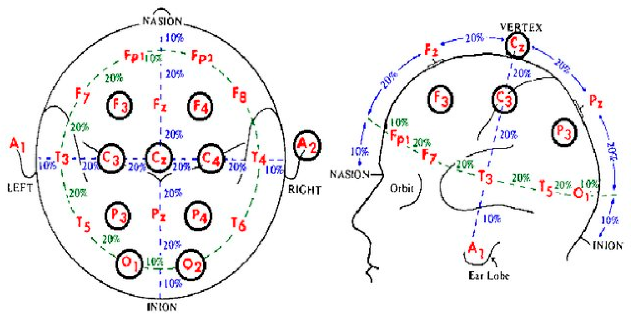
2]. The CHB EEG Signal dataset was taken using the "International 10-20 system of EEG positions", where the spacing of the electrodes on the scalp is dictated by the 10 and 20 values [
1,
2,
3]. The positions of each electrode are referenced by the region of the brain they cover: frontal, parietal, temporal, occipital and the numbering has odd numbers referring to the left half of the skull, even numbers to the right side of the skull, and uses 'Z' for the midline, see
Figure 1 for image [
1,
3].
In recent years there have been many research on seizure event detection and classification using machine learning on EEG signals. The motivation for this is to allow for seizure onset detection (in the pre-ictal state) as well as active seizure detection (ictal). Being able to do these two tasks automonously would give care-givers and patients better alerts to seizure activity to allow for faster and care. Pre-ictal period detection could allow for preemptive care even. Given the number of epilepsy patients worldwide is well into the millions this type of technology could help reduce the impact of this disorder on their lives.
This paper shares the same base dataset with the study [
1], the Pre-Processed CHB EEG dataset, which was created as part of that work. It is based on the original full CHB EEG dataset from [
2]. The study [
1] uses MinMaxScaler for normalizing the data and trained Recurrent Neural Network (RNN), Long Short-Term Memory Network (LSTM), and Bidirectional LSTM models to perform seizure detection. Of the three models, the Bidirectional LSTM was found to perform the best by far, with the LSTM and RNN being very close to each other in performance but clearly separated from the Bidirectional LSTM [
1]. The study [
4] investigated using Support Vector Machine (SVM), Ensemble, K-Nearest Neighbor (KNN), Linear Discriminant Analysis (LDA), Logic Regression (LR), Decision Tree (DT), and Naïve Bayes (NB) models to be considered for automated seizure identification. All of the models trained in [
4] were found to perform fairly close to one another, with KNN slightly edging out the rest on accuracy for un-filtered data and tying LR for the best accuracy with filtered data. In addition, [
5] reviewed using DT, SVM, KNN, Random Forest (RF), and Artificial Neural Network (ANN) models.
This work aims to further test seizure event detection using couples of ML models to classify whether a seizure event is occurring or not. These models were chosen specifically to compare a lighter-weight supervised model like Decision Trees against another supervised but computationally heavier model such as SVM. Similar to [
1], MinMaxScaler normalization was applied to the data after initial detrending and notch filtering for the 60Hz artifact was applied. From here features were extracted and selected using DT feature selection and then modeled using the DT and SVM models. This work differs from [
1] by focusing on supervised learning models, as well as using less of the dataset for training, as this work utilizes an 80-20 training, validation, and test dataset breakdown for Hold-Out based models and also uses 10-fold cross-validation (CV) as well for the models. All analysis and pipeline execution was performed on an Windows 10 desktop machine with an Intel i7-8700 6-core CPU, Nvidia Quadro P2000 GPU, and 16GB DDR4 RAM.
The remaining sections of this paper are structured as follows:
Section 2 presents a comprehensive overview of the dataset, providing specific details. The pre-processing procedure is elaborated upon in
Section 3.
Section 4 outlines the overall machine learning pipeline employed in this study. Moving on to
Section 5, the signal processing methods are described in detail. Additionally,
Section 6 delves into the specifics of feature extraction and section processing. The machine learning methods utilized in this study are elucidated in
Section 7. Lastly, the study's discussion and conclusion can be found in
Section 8 and Section 9, respectively.
2. Dataset
2.1. CHG EEG Dataset
The dataset used in this paper is the Pre-Processed version of the Children's Hospital Boston (CHB) Scalp EEG dataset first published in [
2]. The original CHB dataset consists of EEG measurements from 22 unique individuals consisting of 5 male and 17 female subjects, combining to provide a total of 24 separate "cases" totaling over 900 hours of recorded data [
2,
6]. All of the EEG measurements had a 16-bit resolution and were recorded with a sample rate of 256Hz [
2,
6]. Each case contains multiple captures that, on average, had a 10-second gap between consecutive captures; however, it was variable due to hardware limitations [
2,
6]. Each capture within the dataset consists of 96 channels with 23 "essential channels," which contain the voltage measurements between specific electrodes from the scalp EEG [
1,
2]. The CHB dataset is well regarded due to its large size, containing over 24 cases, over 900 total hours of recorded data in addition to 68 minutes of data during seizures [
1]. Another reason the CHB dataset is well regarded as the 256Hz sampling rate of its recordings allows for analyzing higher frequency aspects of the EEG signals compared to other datasets [
1].
2.2. Pre-processed CHB EEG Dataset
Due to the noisy, imbalanced nature of the CHB dataset, this paper uses the Pre-Processed CHB EEG Dataset, which is a streamlined and balanced version of the CHB dataset provided by the authors of [
1]. The balancing of the CHB dataset was performed by extracting the pre-ictal (leading up to a seizure event) and ictal (during the seizure event) data portions in equal amounts and put into paired files with the same number of samples in each [
1]. The number of EEG data channels was also reduced to 23 essential channels from the original 96 EEG channels. It was discovered in a specific pair of files from the pre-processed dataset, multiple channels were found to be invalid as every data point was identical. While this does not necessarily seem immediately problematic, due to considering MinMaxScaler and Z-Score data normalizations which divide by the range of the data or standard deviation, respectively, this would lead to dividing data by zero. The solution to this was to leave the paired set of files out of the dataset for this work's analysis.
3. Machine Learning Pipeline Overview
The code and analysis presented in this paper were all performed in MATLAB 2022b, and some internal MATLAB functions were utilized. Any special configurational constraints or parameters for built-in MATLAB functions and objects used will be noted.
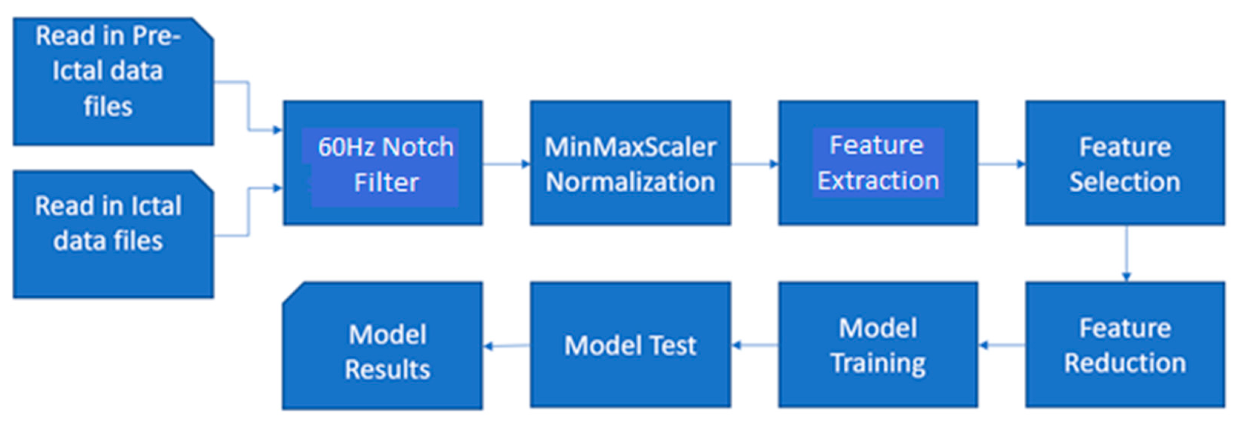
Figure 2 below shows a high-level block diagram and flow of the ML pipeline.
The MATLAB pipeline built and used in this work is that of a very straightforward supervised machine learning model. The first step is reading in and parsing the paired pre-ictal and ictal data files. This data is then put through initial signal processing, including notch filtering out artifacts and data normalization. Next, the two pre-ictal and ictal data are placed together but labeled and undergo feature extraction. Next, feature selection is performed on 80% of the dataset reserved for training. From here, the best number of features are selected for training the model for classification while the rest are reduced. Multiple different values will be tested for the number of features kept. Next, the models are trained. The hold-out DT and SVM models are trained on 80% of the dataset, while a second set of the DT and SVM models are trained using 10-fold cross-validation. Finally, the models perform classification on the test data, and the results are displayed to be analyzed.
4. Initial Signal Processing
The first step taken in the initial preparation of the samples in the dataset after reading in matched pair of files was to apply a second order Butterworth IIR (Infinite Impulse Response) 60Hz notch filter is applied to the presence of any AC power artifacts. The 60Hz notch is used specifically due to the dataset being taken in the United States, where the AC power transmission is dominated by 60Hz [
2]. This was done using the MATLAB filtfilt() function, which applies the filter in both the forward and reverse directions, essentially doubling the order of the filter [
7]. The last step of the initial signal processing in this work was normalizing the data. Two types of normalization were considered in this work: MinMaxScaler and Z-Score normalization. The study [
1] uses MinMaxScaler normalization on the Pre-Processed data set. Following the lead of Deepa and Ramesh, MinMaxScaler was used in this work. Z-Score was considered for the normalization due to the sensitive nature of MinMaxScaler to outliers in datasets skewing the maximum or minimum values used in the normalization. After reviewing the dataset, this was found not to be an issue. This normalization is performed on each channel of a data file separately and is done for each utilized data file.
A commonly used initial signal processing stage for EEG signals not utilized in this work was linear detrending of the signal data. It was found that applying linear polynomial detrending of the data hampered performance for both the DT and SVM models.
5. Feature Extraction and Selection
5.1. Feature Extraction
For extracting features, a window size of two seconds was chosen after reviewing literature and EEG seizure signals [
5]. This means that each window consists of 512 samples for this specific dataset with a sampling rate 256Hz. Different from other works, the windows utilized were overlapped by 256 samples (one second) for extracting features. Each individual channel had ten features calculated for it, and 22 of the 23 channels in the dataset were utilized. This resulted in a total of 220 features being extracted before feature selection and reduction. The base set of 10 features extracted on each channel was chosen based on reviewing literature and is shown in
Table 1 [
5,
8].
5.2. Feature Selection
After feature extraction, the extracted feature data was divided into the training, validation, and test feature sets. The training set was run through a DT feature selection algorithm. This was performed using the existing MATLAB object fitctree, more specifically, the predictorImportance() function from within the object [
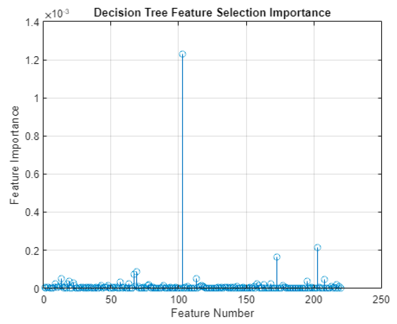
7]. The output of this model was a set of importance values for each feature. Using this importance value, only a select number of features were utilized for training the machine learning models. The process of feature reduction, after feature selection, was implemented such that it is done automatically by the score; however, typically, it was found that the variance (Hjorth Activity) was the most popular of the ten features extracted per channel by far.
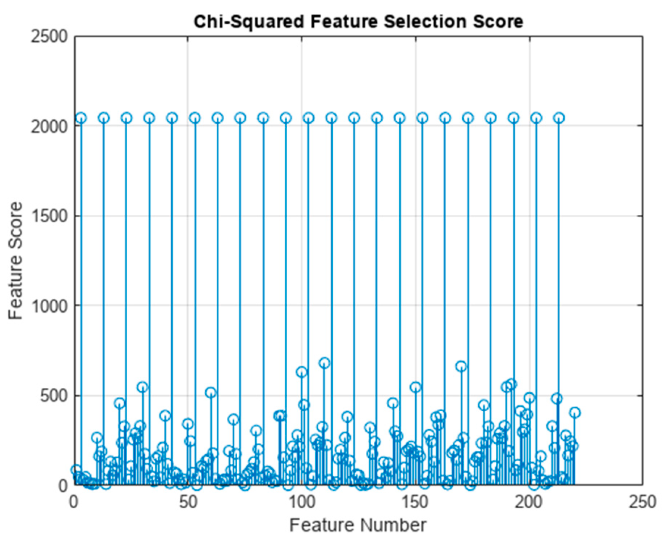
As an alternative method of feature selection, a Chi-Square-based feature selection test was utilized as well. The MATLAB fscchi2 function was used to perform feature ranking using Chi-Squared tests, which resulted in a feature importance score. In terms of which features scored the highest in importance score, this selection method found the variance for every data channel most important.
6. Implemented Models
The two main types of models used to classify ictal versus pre-ictal EEG data were DT and SVM models. Both models were implemented using the existing MATLAB objects: fitcsvm and fitctree, respectively. There were two different dataset division methodologies tested in this work, with the first being 80-20 Hold-Out for training and test data, respectively. The second was using 10-fold cross validation for each model as well. For the hold-out method of dataset division, the MATLAB predict() function was used on the test data to have the model classify the data [
7]. For the cross-validation, the kfoldPredict() function was utilized, which takes the k-fold cross-validated model and gets the classification for the data for each of the k folds [
7].
Two different parameters of the models were experimented with in attempts to optimize performance. The first was changing the number of features utilized for classification in an attempt to discern what number of features input to the model allowed for the best performance. The other parameter experimented with was controlling the depth of the two DT models specifically. This was done using the MATLAB parameter "MaxNumSplits" within the fitctree object [
7]. While there is an explicit "MaxDepth" parameter in MATLAB, this parameter is not usable for cross-validated models [
7]. As such, the depth control was done by limiting the maximum number of branch splits since this parameter was usable for both the hold-out and cross-validated models [
7]. For modifying these two parameters, a grid-like search was performed across different values of each to attempt to find the best-performing models. The number of features was iterated from 8 to 98 in increments of 6. The "MaxNumSplits" was stepped in increments of 50 from 51 to 301. An initial wider run of the grid found the models' performances in the aforementioned ranges to be optimal for the extracted feature set. The two tables below show the results for the models using both DT feature selection (
Table 2) and Chi-square feature selection (
Table 3). With each of the four model types in one of the tables is displayed the three best models found for that type based on accuracy.
Figure 3.
The predictor (feature) importance scores from the DT feature selection. The value with the highest score is Ch11 variance feature.
Figure 3.
The predictor (feature) importance scores from the DT feature selection. The value with the highest score is Ch11 variance feature.
Figure 4.
The predictor (feature) importance scores from the Chi-square feature selection. The variance feature for each of the EEG data channels scored the highest. The actual values of variance scores are infinite due to the way the Chi-Square test works; however, to better visualize this plot any infinite score was set to three times the largest finite value.
7. Results and Discussion
From the results of this work, it is very clear that the Cross-Validated Decision Tree model far outperforms the rest of the models. As expected, the hold-out-based models performed worse than the Cross-Validated ones. Although the one case where a hold-out model outperformed its cross-validated counterpart was for the SVM using DT feature selection. Although this was done with a very low number of features utilized in the model and with more test data would likely lose performance to the cross-validated SVM model. While it was expected the cross-validated DT model would outperform the rest of the models when using DT feature selection, it was interesting that this dataset was still able to outperform the cross-validated SVM model by 20% for the most accurate of each. For sensitivity, precision, and F-Measure (referred to as F-score in [
1]), the cross-validated DT model performs best in as well capturing values of ~90% for each of those values in its top three models of each feature selection method.
It would be of interest for future work to extend testing of the cross-validated decision tree model with different data sets. In addition, adding more features per channel would be interesting to see if model accuracy can be increased further in this regard. Also, there is room for work to be done in testing the effects of characteristics of subjects used for the model from the dataset. For example, it could be of interest to check how the model behaves depending on the gender or age of the subjects within the dataset. Currently, with each subject's data being used, there are 17 female and 5 male unique subjects in the dataset from this work. While this work scratches the surface of the potential for a lighter-weight machine learning model for epileptic seizure detection, such as a DT model, further work should be performed to push for performance improvements and further examine the portability of such a model so it can be used for real-world applications.
8. Conclusions
This work presents four supervised machine-learning models for identifying seizure events. In particular, the cross-validated DT model from this work shows the most promise with an accuracy of 91.17%, precision of 91.97%, and F-Measure of 91.09%. While this does not compare to the over 99.5% reached for each of these values in [
1], this paper did not utilize Deep Learning and Neural Networks and looked into supervised models. The cross-validate DT model shows enough promise for further work to see if it could be improved and utilized for seizure event classification on lower-performance platforms where a neural network and deep learning model would be too computationally expensive. Further work into automatic seizure detection will enhance the lives of epilepsy patients and anyone who suffers seizures often, and the smaller and cheaper the necessary equipment to perform this detection will allow the benefit of seizure detection to more patients.
References
- B. Deepa and K. Ramesh, "Epileptic seizure detection using deep learning through min max scaler normalization," Int. J. Health Sci., pp. 10981–10996, May 2022. 20 May. [CrossRef]
- A. H. Shoeb, "Application of machine learning to epileptic seizure onset detection and treatment," Thesis, Massachusetts Institute of Technology, 2009. Accessed: Sep. 23, 2022. [Online]. Available: https://dspace.mit.edu/handle/1721.1/54669.
- A. Morley and L. Hill, "10-20 system EEG Placement," p. 34.
- A. A. Ein Shoka, M. H. Alkinani, A. S. El-Sherbeny, A. El-Sayed, and M. M. Dessouky, "Automated seizure diagnosis system based on feature extraction and channel selection using EEG signals," Brain Inform., vol. 8, no. 1, p. 1, Feb. 2021. 2021. [CrossRef]
- S. E. Sánchez-Hernández, R. A. Salido-Ruiz, S. Torres-Ramos, and I. Román-Godínez, "Evaluation of Feature Selection Methods for Classification of Epileptic Seizure EEG Signals," Sensors, vol. 22, no. 8, p. 3066, Apr. 2022. [CrossRef]
- A. Shoeb, "CHB-MIT Scalp EEG Database." physionet.org, 2010. [CrossRef]
- "Documentation - MATLAB & Simulink." https://www.mathworks.com/help/ (accessed Dec. 08, 2022).
- I. Stancin, M. Cifrek, and A. Jovic, "A Review of EEG Signal Features and Their Application in Driver Drowsiness Detection Systems," Sensors, vol. 21, no. 11, p. 3786, May 2021. [CrossRef]
- A. Rahman et al., "Multimodal EEG and Keystroke Dynamics Based Biometric System Using Machine Learning Algorithms," IEEE Access, vol. 9, pp. 94625–94643, 2021. [CrossRef]
|
Disclaimer/Publisher’s Note: The statements, opinions and data contained in all publications are solely those of the individual author(s) and contributor(s) and not of MDPI and/or the editor(s). MDPI and/or the editor(s) disclaim responsibility for any injury to people or property resulting from any ideas, methods, instructions or products referred to in the content. |
© 2023 by the authors. Licensee MDPI, Basel, Switzerland. This article is an open access article distributed under the terms and conditions of the Creative Commons Attribution (CC BY) license (http://creativecommons.org/licenses/by/4.0/).


