Model Hierarchy to Reanalyze Results from an Archetypical Experiment on the Kinetics of Heterogeneous Nucleation – the Electrodeposition of Hg on Pt, by I. Markov and E. Stoycheva

We employ hierarchy of models (HoM) with 2, 3 and 4 parameters to reanalyze the nucleation kinetics in the electrodeposition as quantified by n(t) - “the number of nuclei vs. time” data obtained at different overvoltages from precise experiments on electrodeposition of Hg on two different types of Pt-cathodes by Ivan V. Markov and Evgenia Stoycheva [1]. The obtained two scales, nmax and , are used to rescale the original data mapping it on a master curve in coordinates . Our main result is obtained by studying further the dependence of these two scales on the overvoltage (analogue of supersaturation). Surprisingly, for one of the two cathode types - the “hemispherical single-crystal electrode” (as defined by the authors), there is discontinuity in the “ vs. overvoltage” dependence – an almost horizontal jump from 85 to 86 mV accompanied by a change in the slope of the dependence - it is ~ -1 and ~ -0.5 after. For the other cathode - “plane structureless platinum electrode”,  decreases smoothly. Combined, these two behaviors point at the so called “cusp catastrophe”. We compare our findings with published results on protein nucleation.

Keywords:

Subject: Physical Sciences - Chemical Physics

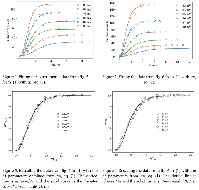
1. Introduction

Following a previous study that employs sigmoid (logistic) dependence to model the so called nucleation data (number of the nuclei formed while the system evolves in time) here we unfold the approach building detailed program that uses a hierarchy of models (HoM) with different number of parameters focused again on nucleation data – that published by Ivan Markov and Evgenia Stoycheva [1]. While finding with high numerical precision the parameters from the different models our study remains neutral with respect to the current achievements in the field of the electrochemical nucleation [2,3] and growth [4] nor do we engage with analyzing the classical theories in the field [5] and how they interrelate with the study of Markov and Stoycheva [1]. Moreover, that we use the models in a straightforward manner and thus not employing classical notions from the nucleation theory such as the induction time and the stationary velocity not seeing them as a result from the analysis.

The thorough and precise study of Markov and Stoycheva provides in our view unique opportunity to analyze the nucleation kinetics in terms of the so called “n-t curves” by counting the number of nuclei on the time-scale of milliseconds. The difference with the previous study [6] and our recent one is that here we do not stop with transforming the data in universal form but we continue further by studying the dependencies of the scales used in this transformation on the parameter that makes the several data sets different – the driving force of the process, the overvoltage. Thus our program acquires its full strength.

It is worth mentioning that Markov and Stoycheva were having in mind the importance of their nucleation experiments for the larger field of vapor deposition on solid surfaces but the true impact achieved by their study could be a subject of a separate study.

2. Hierarchy of models (HoM)

For the reanalysis of the nucleation data by I. Markov and E. Stoycheva [1] we use a set of three models with different number of fitting parameters: α₂₁ is with two parameters, Johnson-Mehl-Avrami-Kolmogorov (JMAKd) – with three, and the Richards model is with four. Anticipating, it is not the number of parameters that improves the fit quality.

2.1. The α₂₁ - model

The so called in the context of two-dimensional crystallization with exhaustion of the initial supersaturation α₂₁ [7] is suited for the purpose of our present study as:

n (t) = n_{\max} \tanh^{2} (2 t / τ_{21})

(1)

and, in fact, represents a further development of the idea behind the model of crystallization in three dimensions describing the evolution of the rescaled size of the growing cube [8] – to obtain a differential equation for the size (in [7] – for the transformation ratio α) based on conservation law for the already exhausted in time t concentration as spread among N equally sized crystals, and on a kinetic law for the remaining part of the concentration, linking the normal growth velocity to the supersaturation raised to a power g. In the index of τ above, eq. (1), 2 stands for the spatial dimension (2D) and 1 stands

g = 1

(the so called growth order). The time t is multiplied by the coefficient of 2 and this comes naturally from the model derivation but it is not “hidden” in the timescale thus keeping the inflection point (t_i, n_i) of the model near the line

n (t) = n_{\max} t / τ_{21}

n_{i} = n_{\max} / 3

(2)

t_{i} = 0.329 τ_{21}

(3)

The last value of 0.329 can easily be mistaken for 1/3 [7].

This is the model with the least number of parameters - n_max and τ₂₁, that we will use at first for rescaling the number of nuclei n and the time t, a program that is already advanced in [6] to study the protein nucleation. The former rescaling operation can be considered also as another formulation of the so called transformation ratio, defined this time as

α \equiv n (t) / n_{m a x}

. Ideally, all the rescaled data should collapse on the same master (universal) curve and the failure of this for some of the data sets should be considered as failure of the model to describe this concrete set adequately. Important aspect in favor of α₂₁ is that it is voiding a “tuning” exponent as the other two from the hierarchy. As a consequence, only α₂₁ has a single master curve n/n_max =tanh²(t/τ₂₁) while for the other two models, JMAK and Richards, the master curves are as many as are the obtained values of the “tuning” exponent - d and q, correspondingly.

Another part of the program, next to [6], is still to be developed in details – to study the dependence of the scales found on the supersaturation. Similar strategy was adopted in [9] to study the cloud condensation nuclei (CCN) as counted in 20 boxes by size at six different supersaturations and then, with rescaling them by the total number of CCN, to map them onto universal distributions, one for each supersaturation, in order to study further the peculiarities of the total number of CCN (but corrected to concentration in this particular case [9]) and how they are linked to the (other) meteo-elements.

2.2. The model of Johnson-Mehl-Avrami-Kolmogorov (JMAKd)

This is a most used model in the theoretical studies in the field of crystallization and nucleation introduced yet in the 1930’s by Kolmogorov [10], Johnson and Mehl [11], and Avrami [12]:

n = n_{\max} {1 - \exp [{(2 t / τ_{JMAK})}^{d}]}

(4)

Note the use of a third parameter in the model, the power d (usually denoted by n but in the present context this would be confusing) - we incorporate it in the abbreviation of the model too to arrive at JMAKd. The initial idea for d is to represent the spatial dimensionality but with the years and with the extensive use in broad range of contexts, see for example [13,14,15], d is considered now more as an additional fitting parameter and its non-integer values are basis for (sometimes lengthy) discussions of why it is not integer as predicted, and why it is varying from experiment to experiment. The link between JMAKd and α₂₁ is studied in detail in [7] and, in particular, it is found that the conversion factor between the two timescales is:

τ_{J M A K 1.725} \approx 1.1 τ_{21}

(5)

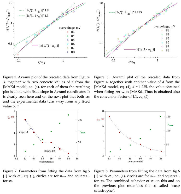
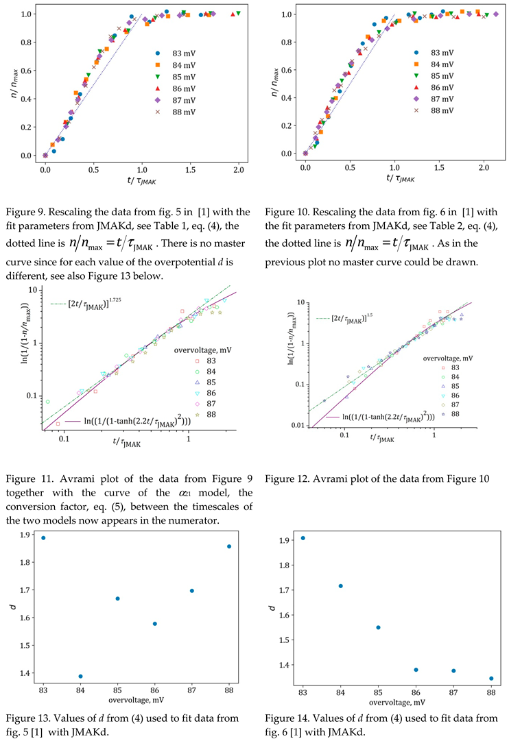
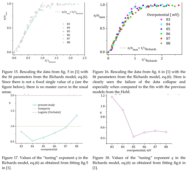
See also Figure 5, Figure 6, Figure 11, and Figure 12 where the concept of the conversion factor is actively used to reconcile the two models. Anticipating, there is no constant conversion factor between the two models introduced so far and the next one – the model of Richards.

2.3. Richards model

This is another general model to study sigmoid growth [16] under the combined action of two feedback mechanisms – positive and negative ones (the form of the differential versions of the two models above is discussed and studied in [7]):

n (t) = \frac{n_{\max}}{{1 + (q - 1) \exp [- (t - t_{i}) / t_{k}]}^{(1 / (q - 1))}}

(6)

what could be easily seen in the differential version of the model:

\frac{d n}{d t} = \frac{k n}{(q - 1)} [1 - {(\frac{n}{n_{\max}})}^{q - 1}]

(7)

Note, that in (7) is used the inverse of t_k – the kinetic coefficient k. Thus, the positive feedback is represented by

k n / (q - 1)

while the negative one is

k {(n / n_{\max})}^{q} / (q - 1)

. This is the value of q that fine-tunes the position of the inflection point of the model and in [16] is found the exact dependence:

n_{i} (t_{i}) = n_{\max} q^{\frac{1}{1 - q}}

. This points at the way of findинг the model’s timescale τ_R – when using the second timescale in (6), the time to the inflection point t_i, which comes into the model only after finding the integration constant from the integration of eq. (7):

τ_{R} \equiv t_{i} q^{1 / (q - 1)}

(8)

to obtain:

α \equiv \frac{n (t)}{n_{\max}} = {(1 + (q - 1) \exp (- K (\frac{t}{τ_{R}} - q^{\frac{1}{1 - q}})))}^{(1 / (1 - q))}

(9)

where K is defined as

K \equiv q^{1 / (q - 1)} t_{i} / t_{k}

and remains the only parameter (next to q) in the non-dimensional version of the model. This non-dimensionalization procedure brings the inflection point of the model on the line

n / n_{\max} = t / τ_{R}

, independent of q and K. Note that the inflection point is the same for any fixed value of q for any value of K and this provides the basis of a further study by considering the connection between the integral curve and the corresponding chaotic mapping in the Richards model. It is worth reminding that the inflection points of the two previous models from the HoM are only close to this line [7].

The Richards model has two commonly used special cases on its own – the logistic model of Verhulst [17] with q = 2, used in the context of nucleation by Nanev at al. [6], and the Gomperz model [14] - with q = 1.

3. Results

After introducing the hierarchy of models (HoM) to be used in modeling nucleation, the first practical step of our reanalysis is to digitize the n(t) data in Figure 5 and Figure 6 from the paper of I.V. Markov and E. Stoycheva published in 1976 [1]. There are numerous tools for digitization ranging from standalone applications as DataThief and ImageJ of NIH, to special packages from the high-level programming languages as R and Python.

We provide in full detail the fitting procedure and the results from it for α₂₁ while the other two models serve more to verify the results from the simplest one in the HoM and for them we give specific details of general interest.

3.1. Fitting with α₂₁ model

3.2. Fitting with the JMAKd model

3.3. Fitting with the Richards model

We do not provide a plot in Avrami coordinates here because again the only master curve would be the one from α₂₁ while in order to plot curves from the Richards model one should chose values not only for q but also for K.

3.4 Summary of the fitting procedure

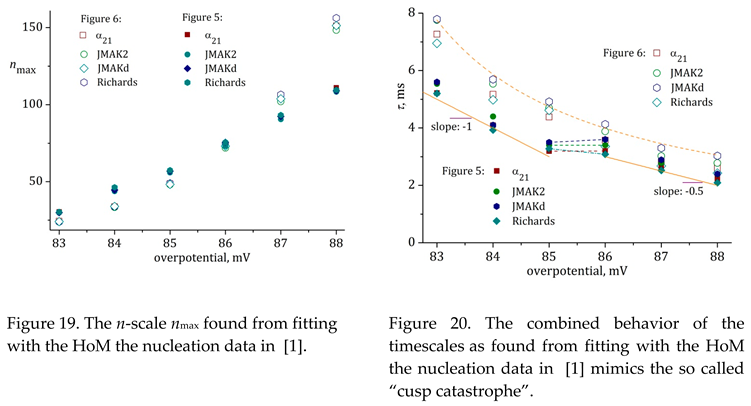
Here we provide the results from the fitting procedure in data format that would permit further comparisons. Thus, in Table 1. are given the values of the parameters as found from fitting the experimental data from fig. 5 of [1] while in Table 2. are listed these found when fitting fig.6 from the same study. Note that the high values of R² obtained cannot discriminate between the models in out hierarchy.

4. Discussion

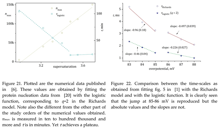
While we are not able to add further argument in the discussion on the existence of an autocatalytic loop in the n(t) dependence next to the one in [6], see also [19], we used a hierarchy of three models with increasing number of parameters to justify our findings.

Note that in the first from the set of two papers [21] I. Markov provides an expression for the saturation density but is not providing an idea of how to treat the data for the timescales nor they are obtained explicitly even as, for example, their inverse values that have the meaning of kinetic factors with attempting the consecutive Arhenius-type plots in order to identify the dependence on the driving force.

5. Conclusions

Our study is intended to remain on a more technical ground providing correct numerical analysis but without of an ambition to judge the theories and their application to experiment. We use a hierarchy of models (HoM) to achieve numerically correct estimation of the two scales describing the phenomenon of nucleation – the maximal number of nuclei and the time-scale for given (and fixed) driving force of the phenomenon. Thus, it is tempting to study the obtained data in a quantitative manner and the main result of this study is the dependence of the time-scales obtained on the overvoltage – smoothly decreasing, for one of the cathodes, and discontinuous for the other. The combination of the two behaviors resembles the so called cusp catastrophe known to the general public yet from the isotherms drawn from the Van der Waals equation above and below T_c.

Acknowledgments

This study was partially financed by grant KP-06-N54/2 from the Bulgarian NSF. VT acknowledges the Mercator Fellowship from the German Research Foundation (DFG) at the Institute for Materials Research and Testing (BAM), and the Glass Department at BAM for the warm hospitality during his stay in Berlin.

Dedication

Our quantitative modelling study provides an original viewpoint on the kinetics of heterogeneous nucleation but also serves as a tribute to the late Ivan Vesselinov Markov (1941 – 2022), who made significant contributions to the fields of Crystal Growth and Nucleation including the books he published [22,23]. It would be unfair to not acknowledge in particular the crucial contribution of the late Evgenia (Zheni) Stoycheva (Armyanova) in obtaining the precise experimental results we reanalyze here.

References

I. Markov and E. Stoycheva, Saturation Nucleus Density in the Electrodeposition of Metals onto Inert Electrodes II. Experimental, Thin Solid Films 35, 21 (1976).
E. Budevski, G. Staikov, and W. Lorenz, Electrocrystallization: Nucleation and Growth Phenomena, Electrochimica Acta 45, 2559 (2000).
A. Milchev, Nucleation Phenomena in Electrochemical Systems: Kinetic Models, ChemTexts 2, 4 (2016).
K. I. Popov, S. S. Djokić, N. D. Nikolić, and V. D. Jović, Morphology of Electrochemically and Chemically Deposited Metals (Springer, 2016).
A. Milchev, Thermodynamics of Electrochemical Nucleation (Springer, 2002).
C. N. Nanev and V. D. Tonchev, Sigmoid Kinetics of Protein Crystal Nucleation, Journal of Crystal Growth 427, 48 (2015).
V. V. Ivanov, C. Tielemann, K. Avramova, S. Reinsch, and V. Tonchev, Modelling Crystallization: When the Normal Velocity Depends on the Supersaturation, arXiv:2304.12402.
C. N. Nanev, V. D. Tonchev, and F. V. Hodzhaoglu, Protocol for Growing Insulin Crystals of Uniform Size, Journal of Crystal Growth 375, 10 (2013).
V. Kleshtanova, V. Tonchev, A. Stoycheva, and C. Angelov, Cloud Condensation Nuclei and Backward Trajectories of Air Masses at Mt. Moussala in Two Months of 2016, Journal of Atmospheric and Solar-Terrestrial Physics 106004 (2023).
A. N. Kolmogorov, On the Statistical Theory of the Crystallization of Metals, Bull. Acad. Sci. USSR, Math. Ser 1, 355 (1937).
W. Johnson and R. Mehl, Trans, in AIME, Vol. 135 (1939), p. 416.
M. Avrami, Kinetics of Phase Change. I General Theory, The Journal of Chemical Physics 7, 1103 (1939).
J. Málek, Kinetic Analysis of Crystallization Processes in Amorphous Materials, Thermochimica Acta 355, 239 (2000).
I. Avramov, Kinetics of Distribution of Infections in Networks, Physica A: Statistical Mechanics and Its Applications 379, 615 (2007).
E. D. Dill, J. C. Folmer, and J. D. Martin, Crystal Growth Simulations to Establish Physically Relevant Kinetic Parameters from the Empirical Kolmogorov–Johnson–Mehl–Avrami Model, Chemistry of Materials 25, 3941 (2013).
E. Tjørve and K. M. Tjørve, A Unified Approach to the Richards-Model Family for Use in Growth Analyses: Why We Need Only Two Model Forms, Journal of Theoretical Biology 267, 417 (2010).
P.-F. Verhulst, Notice Sur La Loi Que La Population Suit Dans Son Accroissement, Corresp. Math. Phys. 10, 113 (1838).
B. Gompertz, XXIV. On the Nature of the Function Expressive of the Law of Human Mortality, and on a New Mode of Determining the Value of Life Contingencies. In a Letter to Francis Baily, Esq. FRS &c, Philosophical Transactions of the Royal Society of London 513 (1825).
C. N. Nanev, On Some Aspects of Crystallization Process Energetics, Logistic New Phase Nucleation Kinetics, Crystal Size Distribution and Ostwald Ripening, Journal of Applied Crystallography 50, 1021 (2017).
C. N. Nanev, F. V. Hodzhaoglu, and I. L. Dimitrov, Kinetics of Insulin Crystal Nucleation, Energy Barrier, and Nucleus Size, Crystal Growth and Design 11, 196 (2011).
I. Markov, Saturation Nucleus Density in the Electrodeposition of Metals onto Inert Electrodes I. Theory, Thin Solid Films 35, 11 (1976).
I. V. Markov, Crystal Growth for Beginners: Fundamentals of Nucleation, Crystal Growth and Epitaxy (World scientific, 2016).
I. V. Markov, Ivan Stranski—the Grandmaster of Crystal Growth (World Scientific, 2019).

Table 1. Parameter values found from fitting fig. 5 from [1] from with the models from the hierarchy. Note that the timescale from the Richards model is not obtained directly from the fit, see eq. Error! Reference source not found., and since no conclusions are drawn based on the values of t_i, t_k and

K \equiv q^{1 / (q - 1)} t_{i} / t_{k}

they are not shown in the tables.

K \equiv q^{1 / (q - 1)} t_{i} / t_{k}

they are not shown in the tables.

over-voltage, mV	α₂₁			JMAKd				Richards
over-voltage, mV	n_max	τ₂₁	R²	n_max	τ_JMAK	d	R²	n_max	τ_R	q	R²
83	30.43	5.22	0.9974	29.9	5.6	1.89	0.9977	30.29	5.20	0.83	0.9967
84	44.61	4.11	0.9937	45.78	4.75	1.39	0.9986	46.28	3.93	0.53	0.9981
85	56.94	3.19	0.9986	56.86	3.51	1.67	0.998	57.36	3.28	0.64	0.9984
86	74.51	3.20	0.9976	75.06	3.61	1.58	0.9992	75.60	3.09	0.79	0.9988
87	92.7	2.62	0.9988	92.37	2.89	1.70	0.9995	93.17	2.52	0.96	0.9989
88	111.01	2.23	0.9974	109.19	2.40	1.86	0.999	109.57	2.09	1.35	0.9983

Table 2. Parameter values found from fitting fig. 6 from [1] from with the models from the hierarchy. Note that the timescale from the Richards model is not obtained directly from the fit, see eq. Error! Reference source not found..

over-voltage, mV	α₂₁			JMAKd				Richards
over-voltage, mV	n_max	τ₂₁	R²	n_max	τ_JMAK	d	R²	n_max	τ_R	q	R²
83	24.41	7.27	0.9966	23.92	7.79	1.91	0.9978	24.12	6.95	1.18	0.9963
84	33.84	5.17	0.9977	33.68	5.69	1.72	0.9978	33.93	4.98	0.93	0.9971
85	48.69	4.38	0.9969	48.97	4.92	1.55	0.9985	48.19	4.62	0.43	0.9987
86	72.78	3.57	0.9890	74.50	4.13	1.38	0.9967	73.07	3.36	0.51	0.9948
87	103.77	2.82	0.9923	106.51	3.30	1.38	0.9993	103.81	2.68	0.54	0.9990
88	151.22	2.60	0.9891	156.27	3.03	1.35	0.9971	151.30	2.43	0.52	0.9958

Disclaimer/Publisher’s Note: The statements, opinions and data contained in all publications are solely those of the individual author(s) and contributor(s) and not of MDPI and/or the editor(s). MDPI and/or the editor(s) disclaim responsibility for any injury to people or property resulting from any ideas, methods, instructions or products referred to in the content.

© 2023 by the authors. Licensee MDPI, Basel, Switzerland. This article is an open access article distributed under the terms and conditions of the Creative Commons Attribution (CC BY) license (http://creativecommons.org/licenses/by/4.0/).

Copyright: This open access article is published under a Creative Commons CC BY 4.0 license, which permit the free download, distribution, and reuse, provided that the author and preprint are cited in any reuse.

MDPI Initiatives

Important Links

Choose an area of interest and we will send you notifications of new preprints at your preferred frequency.

Disclaimer