1. Introduction
The most visible weather/climate trend that can be verifiably attributed to climate change is the persistent increase in global temperatures since the late 1700’s to early 1800’s. The Intergovernmental Panel on Climate Change (IPCC) regarded this causality as
likely with
very high confidence [
1]. More recently, global temperatures have experienced a sudden acceleration over the last 50 years, resulting in overall rate of temperature rise that is unprecedented when compared to the previous 2000 years [
1]. Mean global surface temperature in the most recent decade of 2011-2020 has increased by 0.95 to 1.20°C compared to 1850-1900 and is
very likely projected to rise further up to a total increase of 1.3 to 2.4°C for the period of 2081-2100 when considering an intermediate-low emissions scenario (i.e., Shared Socio-economic Pathway 1 (SSP1)-2.6) [
1].
Projected increases in annual mean surface temperature are not consistent globally or even within a particular country. For example, long-term (i.e., 2081-2100) increases of 2.0 to 3.0°C compared to the recent past (i.e., 1995-2014) are projected in the Midwest and Northeast regions of the United States (US) based on the Coupled Model Intercomparison Project Phase 6 (CMIP6) model simulations using the SSP1-2.6 emissions scenario, while a less extreme increase of 1.0 to 2.0°C is projected for the remainder of the US under the same scenario [
2]. Lee et al. [
2] also show that the projected rise throughout the US in the mid- and long-term scenarios using the higher intermediate-high (i.e., SSP3-7.0) emissions scenario is more highly dependent on proximity to the ocean. For example, consistent with past trends in land vs. ocean surface temperatures, temperatures throughout the entire interior of the US are projected under SSP3-7.0 to increase by a maximum of 3.0°C for the period 2041-2060 relative to the recent past, while areas closer to the coasts are expected to experience a maximum increase of 2.0°C.
In addition to the projected increases in the magnitude of mean, as well as extreme, temperatures, the changing persistence of temperature extremes (i.e., heat waves) is of grave concern. Perkins [
3] describes heat waves as longer-than-normal periods of high temperatures that, in addition to wider contrasts between short-term and seasonal minimum and maximum temperatures, can significantly impact the natural and built environments (e.g., structural integrity of bridges and buildings and damage to pavements and railways) as well as have serious negative implications on human health and mortality [
4]. Multiple studies have assessed past changes in the behavior of heat waves over the last several decades in the US [
5] and globally [
3,
6]. Regarding future projections, the effects of climate change on heat waves will likely be more severe in urban areas due to the “urban heat island” effect. Zhang and Ayyub [
7], for example, projected that the magnitude of heat waves being experienced in Washington, DC, will increase by about 5.7°C by 2100 using the high emissions greenhouse gas emissions scenario or representative concentration pathway (RCP) RCP8.5; the authors also estimated that the frequency and duration of said heat waves will double in the same time frame. Vose et al. [
8] also support projections of more intense heat waves in the future, but also projects a decrease in the intensity of cold extremes. In either case, an important aspect of extreme temperatures, whether hot or cold, is a clear understanding of the influence of climate variability.
As climate change in the form of an increase in global carbon emissions has a clear effect on the increasing trend observed in mean ocean and global surface temperatures, extreme temperatures result from the added variance due to short-term climate variability superimposed on this trend, the basic mechanisms of which are still not well understood [
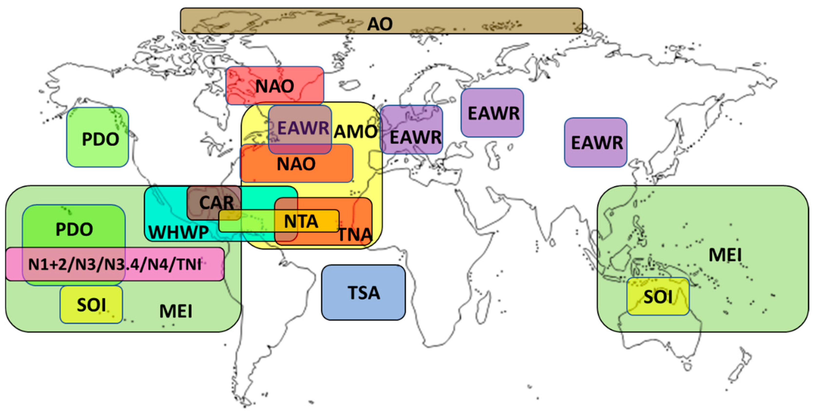
9]. As ocean currents have a major influence on global weather, particularly regarding surface temperatures, the primary modes of climate variability considered in previous studies tend to focus on those that either directly characterize sea surface temperatures (SSTs) (e.g., the Atlantic Multidecadal Oscillation (AMO), the Caribbean index (CAR), and the Western Hemisphere Warm Pool (WHWP) or atmospheric processes that have a strong influence on SSTs (e.g., the El Niño/Southern Oscillation (ENSO), the North Atlantic Oscillation (NAO), and the Pacific Decadal Oscillation (PDO)).
ENSO is the leading mode of interannual SST variability throughout the tropical Pacific Ocean [
10], and as such, has been found to have a significant impact on surface temperature variability in the US, particularly at the subseasonal time scale [
11]. The specific mechanism by which ENSO affects US climate is through the generation of Rossby waves in the western subtropical North Pacific and the subsequent northward and then eastward propagation toward North America. ENSO’s influence on the North Pacific jet stream, particularly during its warm phase (i.e., El Niño) when water located along the equator in the eastern Pacific becomes anomalously warm, causes it to strengthen and extend farther eastward than average; the opposite effect is observed during ENSO’s cool phase (i.e., La Niña). Through the mechanisms mentioned above, ENSO has been found to influence sub-seasonal surface air temperatures within multiple regions in the US: La Niña has been associated with extended periods of colder than normal temperatures in the northwestern and north-central US [
10,
12] during the winter months, while El Niño has been associated with warmer conditions over the Northeast during the winter and spring months and colder conditions over the Southeast during the autumn and winter months [
13]. Various CIs that measure SSTs in different regions within the equatorial eastern Pacific are used to characterize the current phase and strength of ENSO; these include the Multivariate ENSO Index (MEI) [
14]; the Niño 1+2, 3, 3.4, and 4 regions; the Southern Oscillation Index (SOI) [
15]; and the Trans-Niño Index (TNI) [
16]. Refer to
Figure 1 for approximate locations characterized by the ENSO as well as other CIs discussed.
Similar to ENSO, the PDO experiences two phases that are characterized by changes in SSTs and atmospheric pressure in the North Pacific and as well as along the Pacific Coast, though the time scales over which these phases occur are longer. Warm phases of the PDO are characterized by cooler SSTs in the Central North Pacific and warmer SSTs along the western coast of North America [
17]. During the winter and spring months (i.e. November – April), warm phases of the PDO are typically associated with anomalously warm temperatures in northwestern North America and along the West Coast and anomalously cool temperatures in the southeastern US; the reverse pattern occurs during the negative phase.
An area of SSTs along the west coast of North America affected by ENSO and the PDO also includes a portion of what is referred to as the WHWP. The WHWP is the second largest region of very warm water on Earth defined by water temperatures greater than 28.5°C. It includes a small portion of the eastern North Pacific, the Gulf of Mexico, the Caribbean, and the western North Atlantic [
18,
19]. Due to its high temperatures, the WHWP represents a significant source of heat to the atmosphere, which can have a substantial effect on temperatures throughout the contiguous US. Due to the fact that the WHWP encompasses the entire Florida Current, which eventually feeds into the Gulf Stream, the WHWP can impact land temperature along the East Coast as well. In addition, a connection between the WHWP and ENSO through a “tropospheric bridge” has been found to facilitate warmer SSTs in the tropical North Atlantic and WHWP during an El Niño event [
20]. In addition, the CAR [
21], which represents average SST anomalies within the Caribbean and thus is entirely located within the WHWP, can provide additional details in terms of the potential influence of SSTs south of the US on US surface temperatures.
Overlapping a significant portion of the eastern half of the WHWP, there are two CIs that characterize SSTs over a large portion of the tropical North Atlantic while one CI additionally characterizes SSTs in the equatorial and tropical South Atlantic. The North Tropical Atlantic index (NTA) describes SSTs over the portion of the tropical North Atlantic extending from 6N to 18N between 60°W and 20°W and from 6°N to 10°N between 20°W and 10°W [
21]. Overlapping the NTA and extending further east, the Tropical Northern Atlantic index (TNA) characterizes the anomalies of average monthly SSTs over the portion of the tropical North Atlantic extending from 5.5°N to 23.5°N/15°W to 57.5°W [
23]. Further south, the Tropical Southern Atlantic index (TSA) characterizes SSTs from Equator to 20°S/10°E to 30°W [
23]. The NTA and the TNA are especially important in any study of potential mechanisms by which temperatures within the US are modulated by SSTs due to a direct teleconnection between these CIs and ENSO. During the El Nino phase eastward-propagating equatorial Kelvin waves transport tropospheric temperature changes from over the eastern and central tropical Pacific to the tropical North Atlantic [
24]; an eastward shift and increased variability of ENSO due to global warming have been identified and may have significant effects on extreme SSTs and SST variability within both regions within the tropical Atlantic [
25]. As an additional mechanism by which all three CIs may affect US surface temperatures, high SST anomalies within the tropical Atlantic (i.e., a region limited to SSTs of 28.5°C or greater) have been found to generate convection over the Caribbean and anticyclonic circulation anomalies in the upper troposphere over the Gulf of Mexico and Great Plains, resulting in enhanced subsidence, reduced cloud cover, and higher surface warming for large parts of the US [
26]. As such, these conditions were found to be associated with a higher frequency of heat waves for much of the US east of the Rocky Mountains.
CIs that characterize atmospheric patterns over portions of the northern Atlantic Ocean have also been found to have significant impacts on US weather and temperatures. The AO [
27], for example, is a large-scale climate pattern that describes the strength of counterclockwise-circulating winds at approximately 55°N latitude. A belt of strong winds at this latitude strengthen during the positive phase of the AO, which results in colder air being confined to the polar regions. Warming during the positive phase of AO has been found to be especially significant over the eastern third of the US during the winter months of January to March [
28]. The negative phase is represented by a weakening of the wind belt, which allows the colder air to penetrate southward into the midlatitudes. The NAO [
29,
30], which is closely linked with the AO, characterizes atmospheric pressure patterns over Greenland and those associated with the Subtropical High near the Azores. The positive phase of the NAO is linked to below-average pressures over Greenland and the North Atlantic and above-average pressure over the Azores as well as the eastern US and western Europe; opposite conditions are observed during the negative phase. Such pressure patterns tend to cause the eastern US to experience above average temperatures during strong positive phases of the NAO and below average temperatures during strong negative phases [
31]. Volkov et al. [
32] have also demonstrated that large-scale heat divergence throughout the North Atlantic resulting from these atmospheric patterns results affects the temperature of the Florida Current, which can also have some effect on land surface temperature along the East Coast of the US. A third CI, the Eastern Asia Western Russia index (EAWR) [
28], also characterizes atmospheric pressure anomalies within the central North Atlantic as well in Europe, northern China, and near the Caspian Sea. Though previous studies regarding a potential connection between the EAWR and US land temperatures are sparse, there is evidence of a potential link with precipitation in portions of the US [
33]; therefore, for the sake of completeness, the EAWR was considered in the current study.
Encompassing a large area of the North Atlantic that significantly overlaps regions that are characterized by the WHWP, NTA, TNA, NAO, and the EAWR, the AMO [
34] provides a weighted average of SSTs from the Equator to approximately 70°N. Average SSTs in this region have been found to vary on a low-frequency multi-decadal time scale. Due to its potential contribution to the PDO [
35] and overall influence on northern hemisphere surface temperatures [
36], particularly over North America and Europe, the AMO represents yet another CI that must be considered in any study on the effects of climate variability on temperatures in the US.
Based on the discussion above, the present study consists of two parts. The first part attempts to link long-term average monthly mean, minimum, and maximum temperatures throughout the US to any one of a comprehensive set of CIs (see
Table 1) in order to compare potential links between mean and extreme temperatures and the modes of climate variability represented by the CIs tested. The CIs considered include those characterizing atmospheric activity (i.e. pressure and height anomalies) and SSTs over and within portions of the central and northern Pacific and Atlantic Oceans and the Caribbean (see
Figure 1 for approximate locations) and for which strong links to surface temperatures within the US have been previously identified or are plausible. The results would assist in identifying the existence of spatial patterns over which specific CIs exhibit a dominant link to long-term mean and/or extreme surface temperatures. Such information would contribute to a better understanding of the long-term variability in mean temperature as well the intensity and frequency of heat waves. The data and methodology used to assess these links are discussed in
Section 2, while the results of the analyses are provided in
Section 3. A discussion of how the final results fit or diverge from the narrative formed by previous studies as well as how they are or are not consistent with similar previous analyses related to precipitation and sea levels is provided in
Section 4. Final concluding remarks are reserved for
Section 5.
4. Discussion
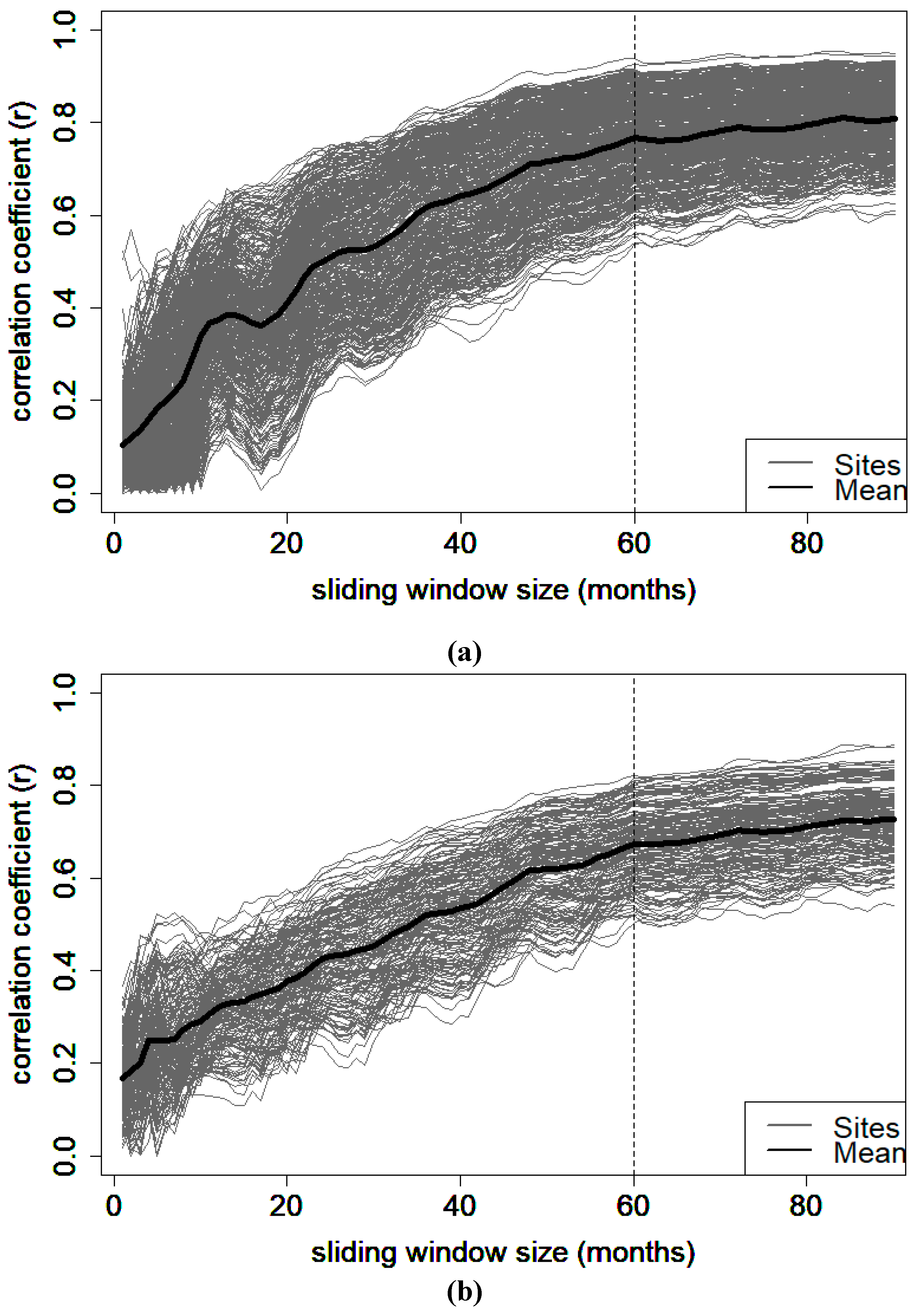
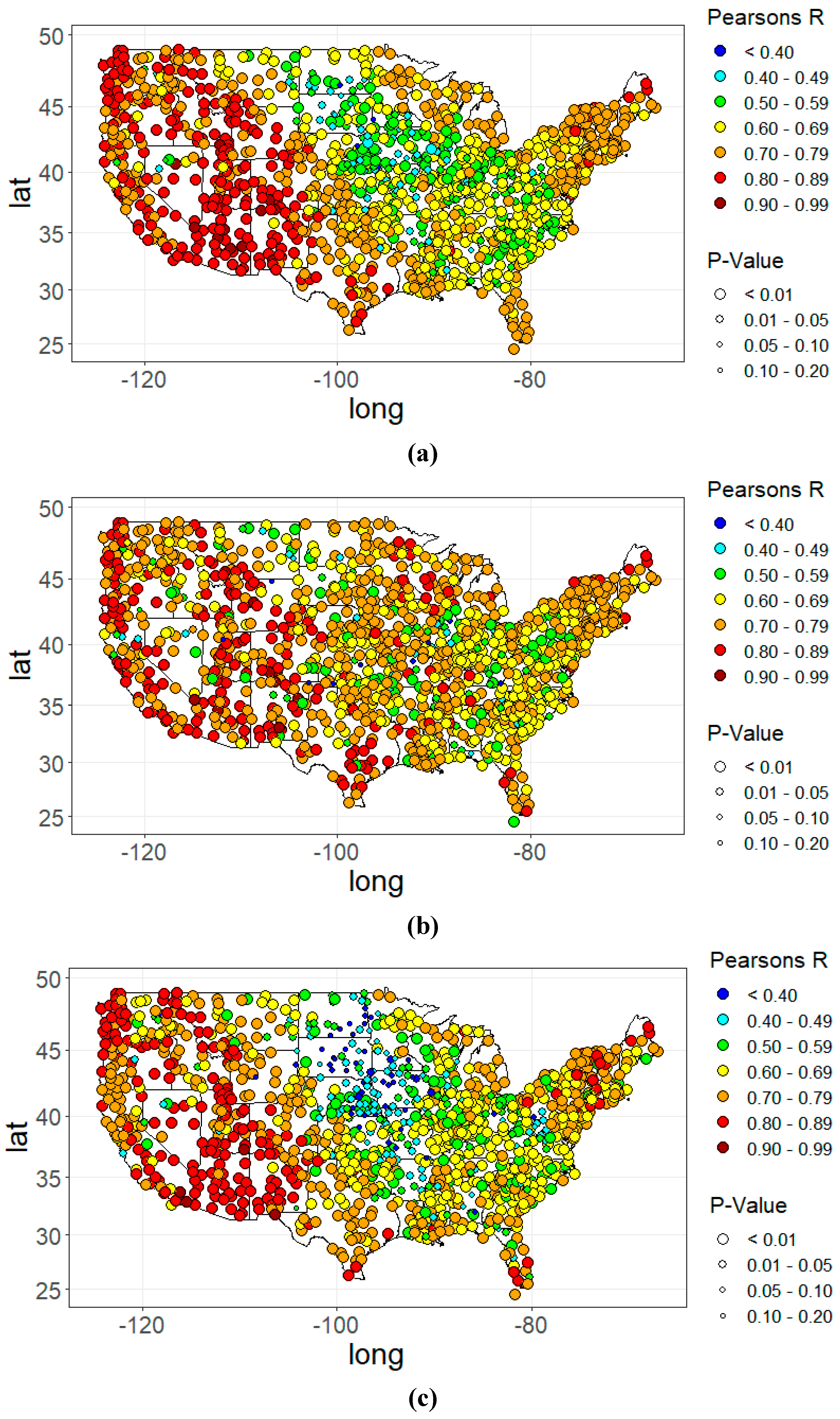
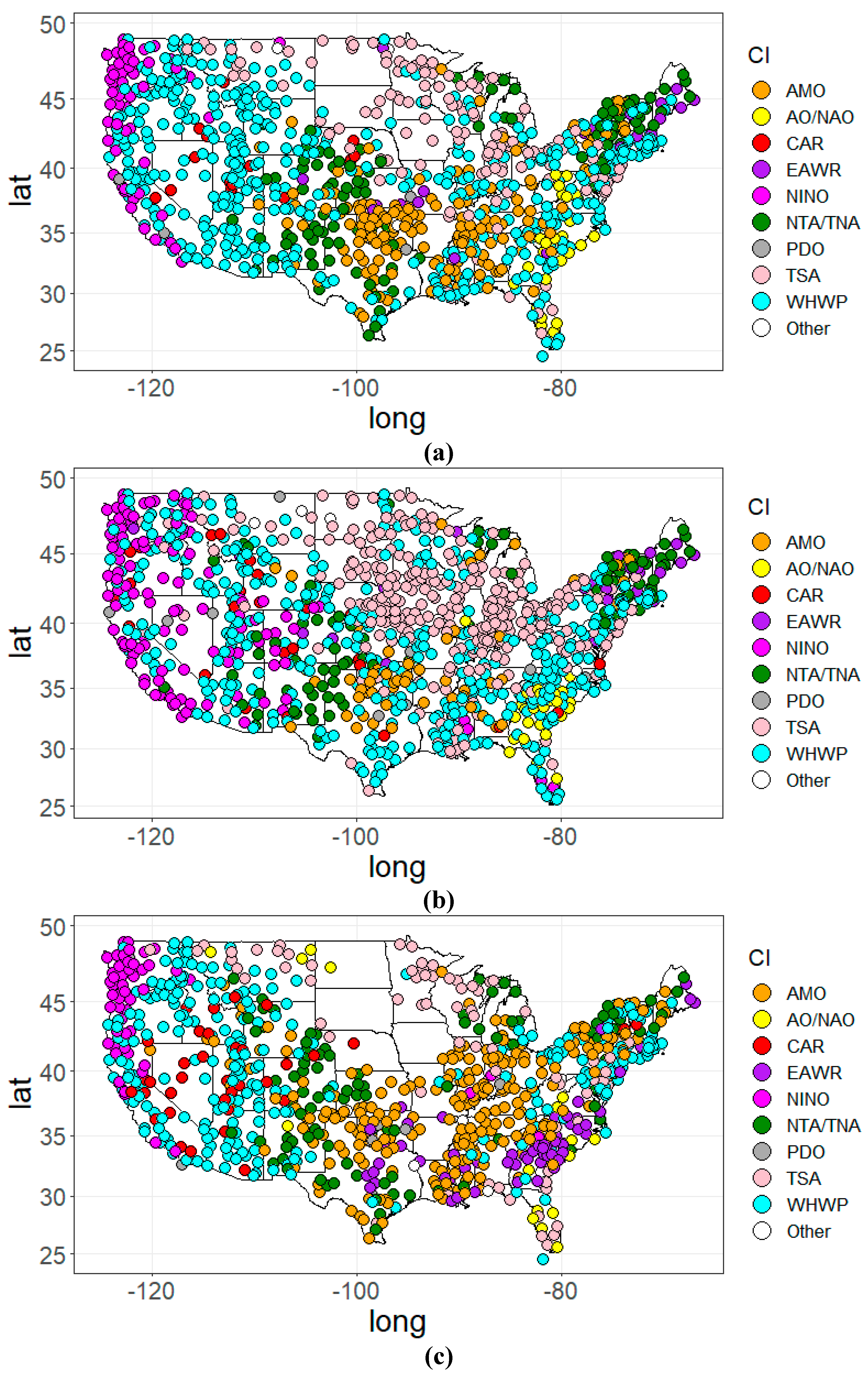
Correlation analyses between long-term monthly mean, maximum, and minimum surface temperatures and several climate indices (CIs) were performed over the period of record 1948–2018 in an attempt to identify spatially consistent links between various manifestations of climate variability and surface temperatures at sites located throughout the US. Analysis of long-term (60-month) averages of each temperature dataset revealed dominant links by a few prominent CIs: namely the ENSO CIs along the West Coast, the WHWP throughout the interior western half and a large portion of the eastern half of the US, the AMO in the southern Great Plains and Midwest, the NTA and TNA in the southern Great Plains and Northeast, the TSA throughout the northern Great Plains and Midwest, and the EAWR in the Southeast and Northeast. These results are consistent with mechanisms identified in the literature as described previously and serve as a basis from which to identify potential CIs that deserve additional research regarding their effect on weather in a particular region of the US.
The significant effect of SST variability within the Pacific Ocean and Gulf of Mexico on temperatures throughout the western half of the US is confirmed through the dominant correlations between long-term mean, maximum, and minimum temperatures and the CIs characterizing ENSO as well as the WHWP. The influence of ENSO’s effect on Rossby waves from the west is especially obvious at sites located along the entire US West Coast where ENSO is most dominant.
The dominant influence of SSTs either directly to the west or south declines significantly slightly as one moves slightly east of the Rocky Mountains into the Great Plains. A strong link to the AMO manifests itself for all temperature datasets within the southern Plains. This AMO region expands to the east when considering mean temperatures and further expands to the northeast when assessing the AMO’s potential link to monthly maximum temperatures. The dominant link of northern (in this case tropical northern) Atlantic SSTs to all temperature types in the southern Plains is further confirmed by the added dominance of the NTA/TNA on the western border with the Rocky Mountains. In contrast, the northern Great Plains is dominated by the TSA for all temperature types, though the significant of these links progressively decreases moving from minimum to mean and on to maximum monthly surface temperatures. Both links to the tropical Atlantic SSTs (and potentially to the AMO, though the AMO covers a much larger area that extends far north of the tropics), particularly in the case of maximum temperatures, supports prior research that has shown a significant effect of tropical Atlantic SSTs on the incidence of heat waves throughout the Great Plains [
26], though it is interesting to note that the current suggest that this influence may extend much further to the east and northeast.
Dominant links associated with atmospheric behavior over north of the tropical Atlantic was limited the Southeast and portions of the mid-Atlantic as well as the extreme Northeast when considering all temperature types. Links with the AO and NAO were present in the Southeast and within a small area near the Shenandoah Valley in all cases as was a link between the EAWR and temperatures in the extreme Northeast. When considering monthly maximum temperatures, a strong link with the EAWR also manifested itself over a large portion of the Southeast that included the states of Georgia and North and South Carolina. Such links are supported by prior studies previously mentioned [
28,
29,
30,
32], especially proximity to the coast.
Based on the results of the current study with regard to surface temperature,
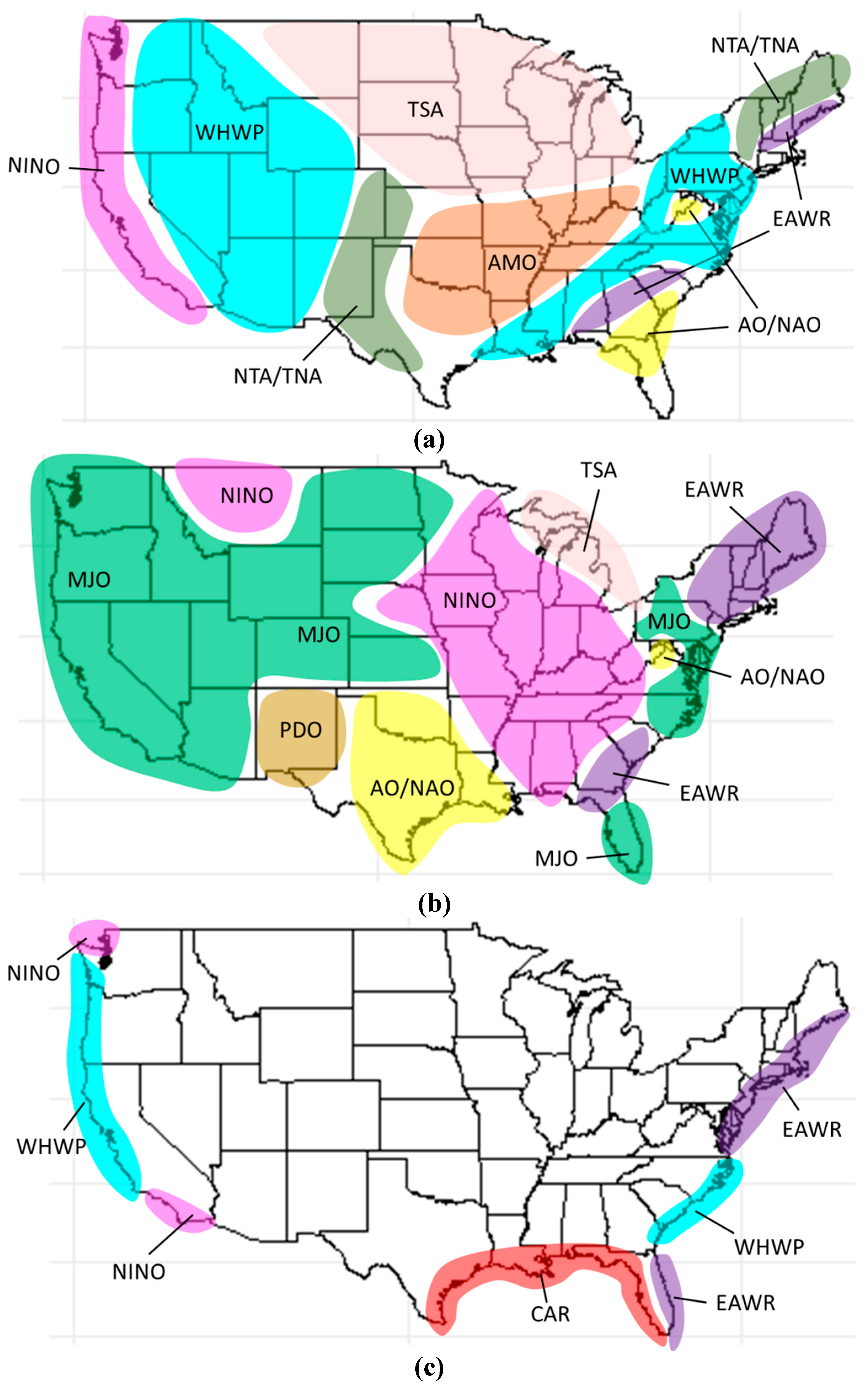
Figure 6a provides a clearer, but more general, representation of approximate regions over which the CIs mentioned above were dominant. The regions as shown do not depict the more detailed differences observed between long-term mean, minimum, and maximum monthly temperatures, but merely provide an overall assessment in order to guide future research and as a way to compare to similar analyses performed in prior studies. To this end,
Figure 6b and
Figure 6c present similar maps that provide general assessments of results from prior studies focusing on long-term monthly precipitation [
33] and sea levels [
44], respectively. One key difference that should be noted here is that due to the shorter period of record over which data on the Madden-Julian Oscillation (MJO) is available, the MJO was not considered in the current study; as a result, comparisons with between
Figure 6a and
Figure 6b for the western half of the US cannot be made based on the results presented, though additional results in Giovannettone [
33] did indicate a strong link to ENSO when longer lag times were considered, which is consistent with some of the findings here and in Giovannettone et al. [
44], though no lag times were used in both instances.
Unlike in the western half of the US, some informed comparisons can be made throughout the eastern half. The apparent links between atmospheric behavior over the northern Atlantic (i.e., AO/NAO and EAWR) and weather over the Northeast, the Shenandoah Valley, and a large portion of the Southeast is evident for both temperature and precipitation. Further evidence of potential teleconnections with the EAWR are evident in the fact that it represented the dominant CI with regard to long-term mean sea levels along both the Northeast and Southeast coastlines (
Figure 6c). These results suggest that this potential weather and sea level connection to the EAWR should be studied in further detail as literature on this topic is extremely sparse if not nonexistent. The EAWR also presents an opportunity to identify teleconnections between weather in parts of the US and weather in other regions characterized by the EAWR (i.e., Caspian Sea, Europe, and northern China).
5. Conclusions
There is a lack of knowledge and data to identify communities and locations most at risk from extreme temperatures, particularly with respect to extended period of high temperatures (i.e., heat waves), which can have detrimental effects on human health and the natural and built environments. Such knowledge is crucial to make planning decisions related to decreasing vulnerability and increasing resilience both now and in the future, particularly in the face of climate change. Due to the direct projected effects of climate change on mean and extreme temperatures, it is essential to be aware of the underlying mechanisms related to climate variability that can be linked to short- and long-term fluctuations in temperatures, on top of which the projected effects of climate change can be superimposed.
In an attempt to understand some of the underlying mechanisms related to long-term temperature variability, potential links between several climate indices (CIs) and long-term average mean, minimum, and maximum surface temperatures were assessed during the study period 1948–2018. The CIs considered in the current study either characterized SSTs over portions of the eastern Pacific Ocean, the tropical Atlantic Ocean, and the Gulf of Mexico and Caribbean, or atmospheric behavior in terms of height and pressure anomalies over the northern Atlantic Ocean. It was found that the Western Hemisphere Warm Pool (WHWP), which characterized SSTs south of the US, exhibited the most widespread dominant link with mean and extreme temperatures throughout the western US and portions of the East. Dominant links with ENSO were also identified, though these were limited to a thin region extending along the entire West Coast. Dominant links to SSTs southeast of the US (as characterized by the AMO, NTA, TNA, and TSA) within the northern and southern tropical Atlantic Ocean were found in all cases throughout the northern and southern Great Plains as well as the Great Lakes regions. Temperatures within large portions of the Northeast and Southeast were linked to changes in atmospheric patterns over the northern Atlantic as characterized by the AO, NAO, and EAWR. This is not surprising as the locations of atmospheric conditions characterized three CIs are adjacent to each other, though previous research has focused on the AO and NAO while devoting little attention to the EAWR. Proposed ideas with regard to potential mechanisms were proposed, but additional research is required to confirm the level of causality regarding all links that were identified.
The results from the current study were then compared to similar results from previous studies that were focused on long-term precipitation and sea levels in order to determine the extent to which similar links were found. The dominance of the WHWP and ENSO in the West was shared by the temperature and sea level analyses, while the MJO revealed stronger links with precipitation. An additional similarity that was found was the dominance of the EAWR in the Northeast for both weather parameters as well as long-term sea levels. These results, as well as the current lack of research related to any effects of the EAWR on weather and climate in the US, stress the need for future research focused in this area.
