1. Introduction
There are approximately 2 billion people around the world whose water supply is dependent on glacial meltwater [
1]. A glacier can provide a vital multiannual buffer as a valuable natural water reservoir, especially in drought-prone regions [2, 3]. In many parts of the world, large rivers originate from mountain areas where snow and glaciers store a large quantity of fresh water. A total of 75% of the world's freshwater is stored in glaciers, 99.5% of which is found in Antarctica and Greenland (IPCC, 1996). Their influence can be seen in several important areas such as flood control, sediment transport, irrigation, water consumption, and hydroelectric generation because they control the hydrological regime in mountainous areas. There are different time scales on which glaciers play the role of water stores and regulators of the hydrological regime, short-term processes e.g. flood on a daily or sub-daily basis, medium-term processes, seasonal and inter-annual fluctuations in hydrological regimes in glaciated areas, and long-term processes changes in sea level [
4].
In the past decade, glaciers in most parts of the world have been retreating, resulting in a wide range of implications, from global effects on sea levels and ocean systems to regional [
5] and local effects on catchment hydrology [
6]. Glaciers have been retreating strongly [
7] and are expected to continue doing so throughout the 21st century [
8], their role in the water cycle will change. It appears that 'peak water has already passed in many basins around the world, indicating a recent change from glacial to naval-pluvial regimes' [
9]. In addition to impacting millions of people's water supply, this could also increase the likelihood of natural hazards, increase hydro-political tensions [
10], and undermine the reliability of many ecosystems impacted by glacial meltwaters [
11]. The change in glacier runoff due to glacier retreat is a concern, especially in areas where glacier runoff is an important source of water for agriculture, industry, and municipalities. It is therefore essential to investigate the hydrology of glaciers at these watersheds. Demographic pressure, changing climate, and glaciers' shrinking under climate change pose a serious threat to water security in the Andean region [
12]. Recent studies have demonstrated glacier retreat and thinning in central Chile over the twentieth century, with an average estimate of 12.8% of glacier area loss over the 51 years between 1945 and 1996 [
13]. With over 7 million inhabitants, the Santiago region uses 70 to 90 percent of its agricultural water from the Maipo River [
14]. Meltwater is essential for both agriculture and urban centers of growing demographic and economic importance during the summer. Competition for water allocation grows as water use increases as the population increases and the country becomes more industrialized [15, 16, 17]. Pellicciotti et al. [
18] reviewed the recent status of Chilean glaciers and found that the central Andes glaciers, specifically Juncal Norte, Juncal Sur, and Olivares Gamma glaciers, which are in the Maipo catchment, have been shrinking rapidly since 1955. Their area has been declining by 2.4%, 10.9%, and 8.2%, respectively. Over the next century, water use is expected to rise [
19] on the other hand temperature trends at locations throughout the region [
20], including the upper river basin, show that summer and winter air temperatures have increased statistically significantly since the 1970s [
21]. An increase in air temperature is likely to influence the summer snowmelt phase, by enhancing it, and the winter precipitation phase, by reducing the amount of snow accumulated at the start of the melt season [
22].
It has been shown by Carrasco et al. [
20] that the snow line in central Chile has risen by 127 measures over the last quarter of the twentieth century. There has been great progress in glacier modeling encyclopedically in the once many times [
23]. Indeed, however all these approaches produce harmonious results at the global position, their indigenous and original results are subject to lesser misgivings [
24]. Several reasons contribute to this, similar to the high position of abstraction of the key processes, the need to spatially fit the model parameters, and the query in the boundary and initial conditions [24, 25]. The maturity of models doesn't include ice dynamics, has no anterior ablation [
26], and warrant modulation of the mass balance face by debris cover and snow redivision (winds and avalanches). Among the available models, only one [
24] was suitable to give estimates of once glacier volume changes and there's no open-source interpretation of these models.
The use of a spatial glacier model is pivotal to constructing a model for assaying changes in glacier mass over time. To negotiate this, automatic initialization styles are needed, and several different approaches have been used in the development of hydrological models to integrate the snow and ice melting processes [27, 28]. Among the models, Snowmelt Runoff Model (SRM) and the HBV model are extensively used to study the effects of climate change on glaciers grounded on meteorological data, satellite data about snow cover, and climate scripts [29, 30, 31].
In this paper, we probe how including glaciers in a hydrologic model impacts its performance and enhances the being models. The original idea was to develop a completely distributed physically grounded glacier hydrological model able to develop the mass balance process. Accordingly, a glacio- hydrological model tool is planned to develop as an extension to the being mHM (The Mesoscale Hydrologic Model) with post-processing and visualizations. The hydrological model (mHM) is developed in the Fortran programming language and due to time and resource constraints, the original idea was changed from developing the glacier module into mHM to assaying glacier hydrological models and understanding the counteraccusations of the glacier model being implemented into mHM.
It's within the environment of taking robust representations of glaciers in hydrological models since glacier melt is an important contributor to sluice inflow. This thesis seeks to contribute to the understanding of how dependable models that have minimum data demands, similar to MATILDA (Modeling Water coffers in Glacierized Catchments), can be applied successfully in different catchments and how the full query of their catchment runoff protrusions can be reckoned for and understood.
This thesis explores how including glaciers in a hydrologic model impacts the model's performance and enhances existing hydrologic models. An open-source tool called MATILDA (Modeling Water Resources in Glacierized Catchments) is used to analyze the glacier catchment and compare it with a hydrological tool mHM using grid cells as the primary hydrologic unit and is spatially explicitly distributed. The purpose of this analysis is to gain insight into the differences between running a snow melt module and a glacier melt module. As case studies, the evolution of the glacier in the entire mountainous area of the Maipo basin in Santiago, Chile is investigated using regional climate scenarios.
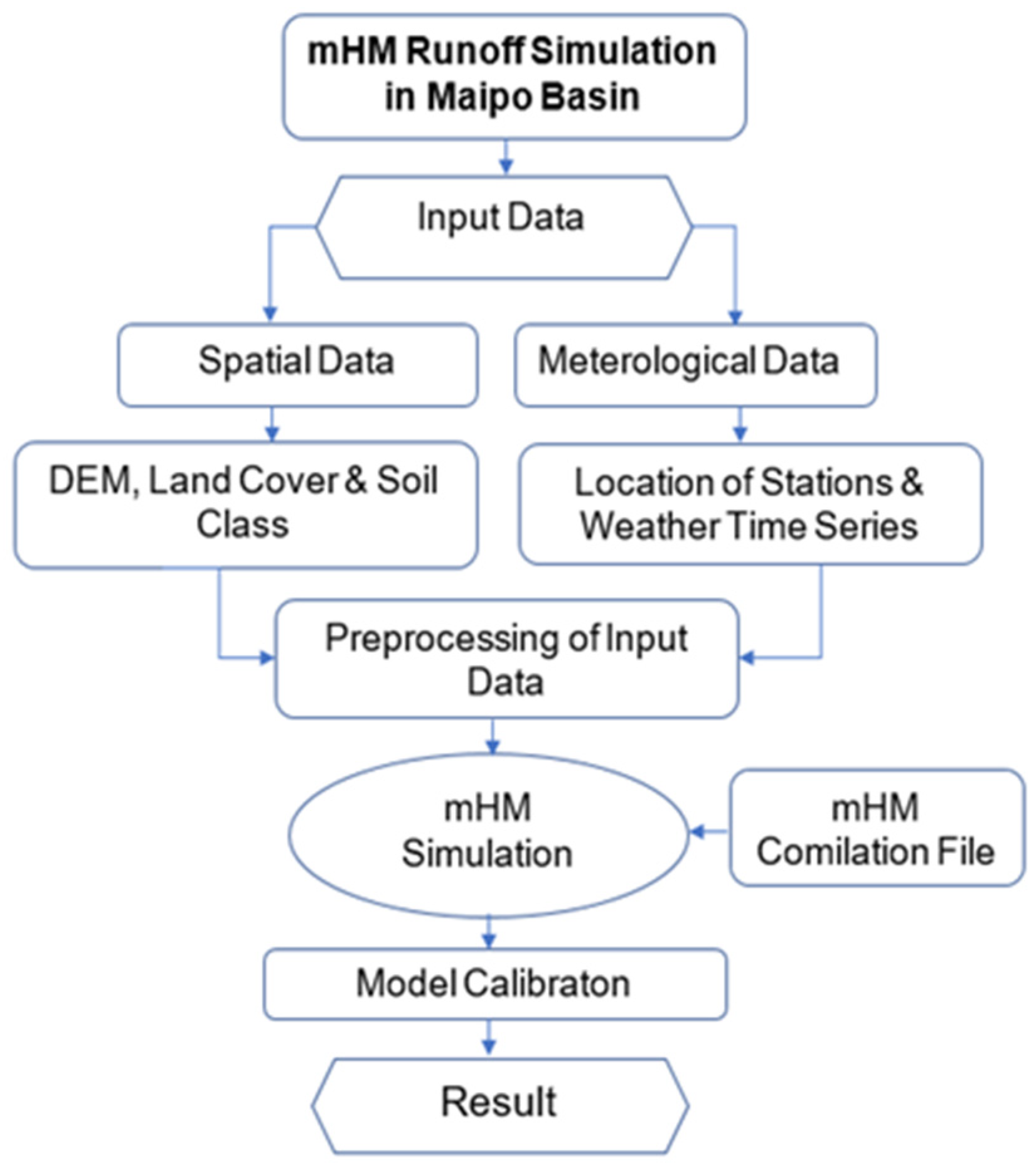
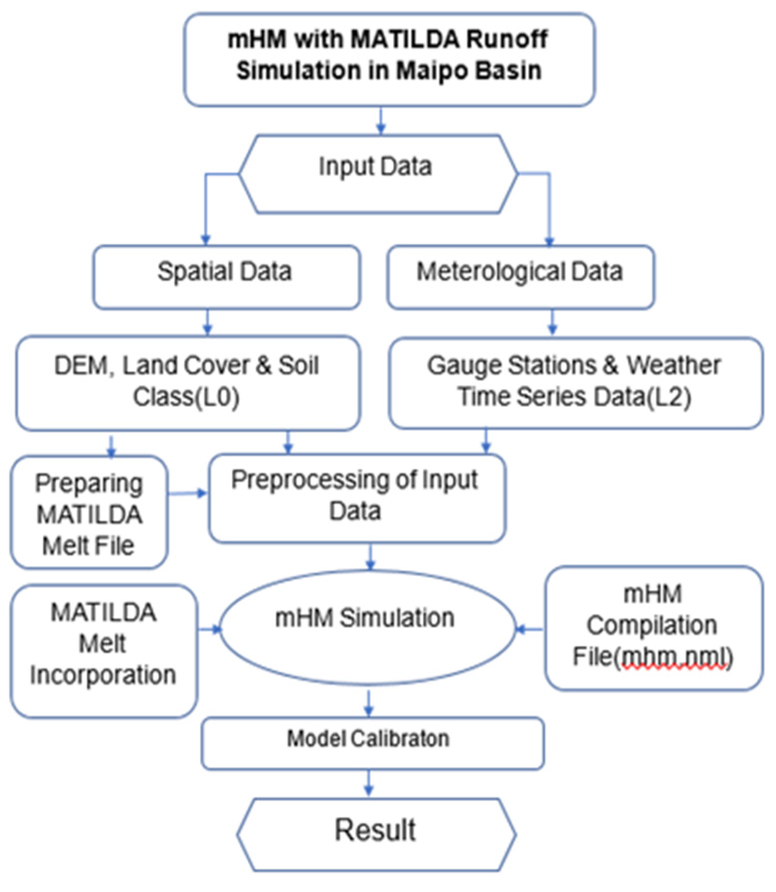
The initial objective of the thesis is divided into different targets. Firstly, mHM is performed for the whole Maipo basin as per the workflow described in
Figure 7 and then MATILDA (Modeling Water Resources in Glacierized Catchments) is performed for the whole Maipo basin. To integrate MATILDA melt into mHM, a pilot sub-basin is performed with the MATILDA model, and then the output melt is incorporated into the mHM model as per the workflow described in Figure 9 and then the mHM model runs again with the MATILDA melt.
2. Materials and Methods
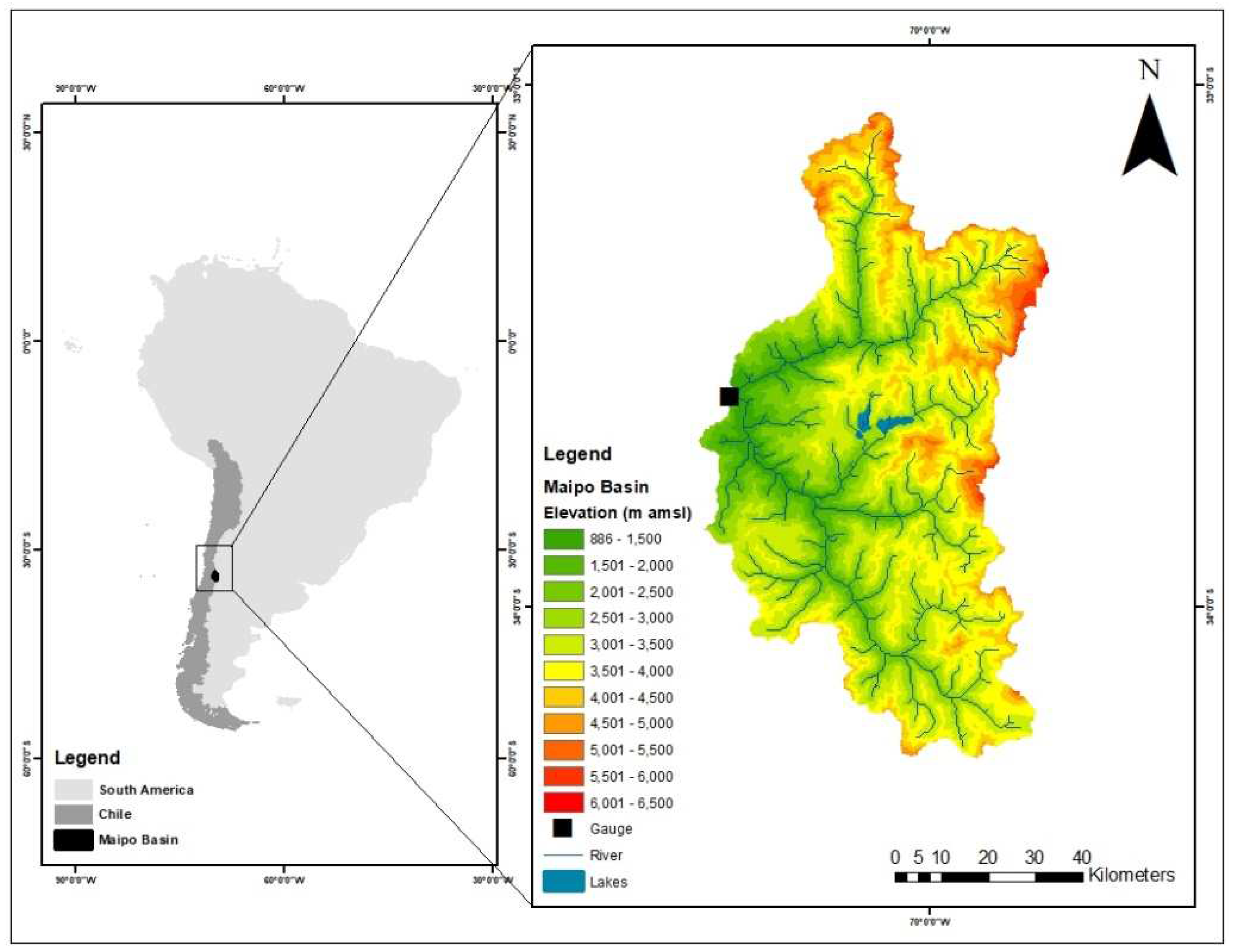
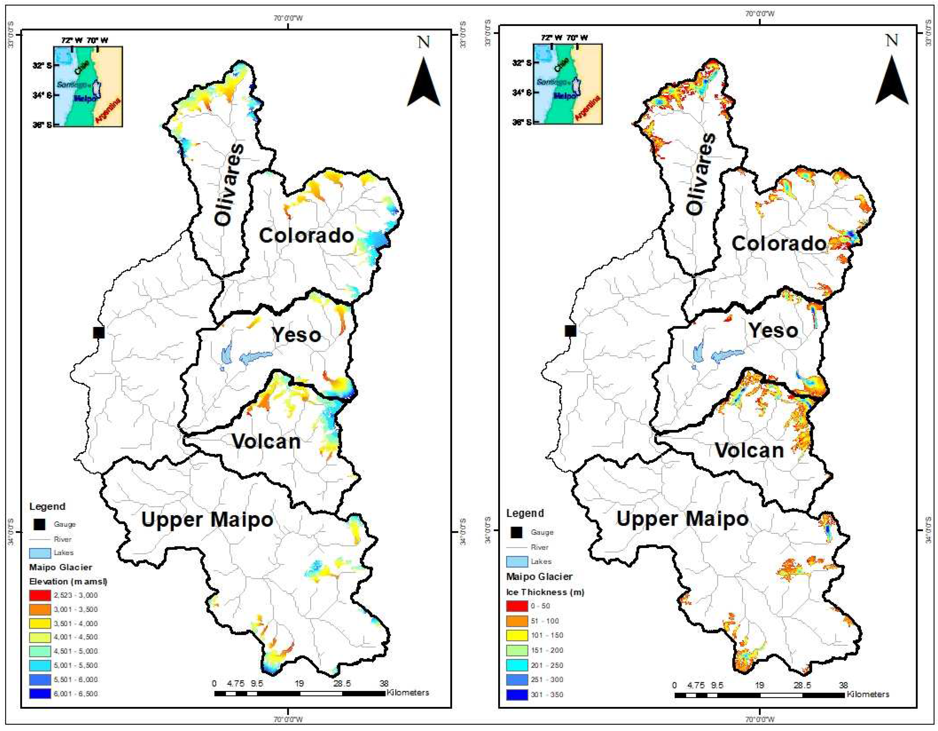
The study areas for this research consist of the catchment area of the Maipo River Basin Rio Maipo En El Manzano catchment as shown in
Figure 1, with the gauge id “5710001” located in Central Chile close to a small town El Manzano along the river, about 15 km upstream of Santiago. The basin is located between the latitudes 32.92° to 34.29° and, longitude 69.77° to 71.63°, with an area of approximately 4839.04
and altitude, varied between 890 m a.s.l to more than 6500 m a.s.l. Around only 10% of the area is below the 2000 and 40% is below the 3000 m a.s.l. The average flow at the El Manzano gauge station was 120
from 1980–2013 and it is a fundamental natural resource for cities, including the Chilean capital Santiago, whose population comprises 40% (~7 million) of the country.
The Maipo River Basin contains high mountain basin areas and a total of 364 of the area was covered by glaciers, which accounted for approximately 8% of the area. (1980–2013). According to the Chilean glacier inventory, approximately 1000 individual ice bodies could be found in this region, including ice bodies with debris-free or debris-covered surfaces, and rock glaciers. This represents approximately 1.7% of the total area of Chile covered by glaciers. Glacier surfaces range from 21 (Juncal Sur Glacier) to 0.01 . The mountain area of the Maipo basin is further divided into 5 sub-basins to investigate glacier modeling. The Upper Maipo basin has the highest basin area and lowest maximum elevation compared to other basins. The Colorado Basin has the maximum elevation of the glacier.
2.1. Meteorological Data Preprocessing
The meteorological data used in this application is obtained from the ERA5 [
32] and CAMELS-CL database, for the basin Rio Maipo En El Manzano (5710001) where the station is installed. The CAMELS-CL website provides information from S16 fluviometric stations throughout Chile, including daily flow data as well as daily meteorological data. The meteorological data were obtained from the ERA5 dataset with a resolution of 27-28km, and the observed discharge was obtained from the gauge station located at CAMLES Cl from 2011-2018. According to
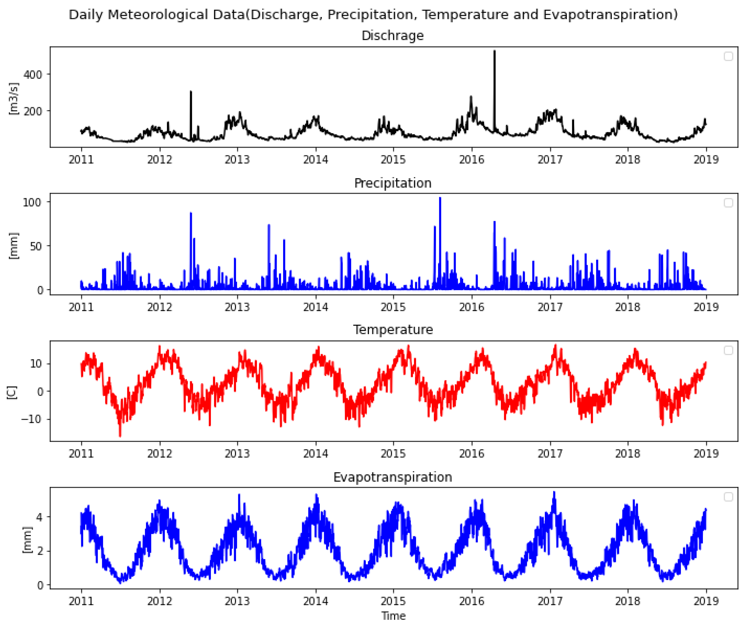
Table 1, data from 2011-2018, the average discharge was 77.41
, so it has decreased when compared to 1980-2015. In autumn 2016, the maximum discharge was recorded at 526
, which is unrealistic considering the precipitation during that period shown in
Figure 2, so it may have been due to radiation or sunshine, or even an outburst of catchment storage.
The mean precipitation is recorded as almost 3 mm from 2011 to 2018 with a maximum of 104.3 mm. Over the period 2011 to 2018, maximum and minimum temperatures ranged from -16 to +16 C°, with an average of 2.7 C°. A mean evapotranspiration of 2.04 mm was recorded between 2011 and 2018, with a maximum of 5.43 mm.
According to
Figure 2, discharge showed two peaks during the Autumn of 2012 and 2016, for the first peak precipitation is also showing a high rise during that time, and the second peak didn't show a strong rise from the precipitation. There is a maximum rise in precipitation during the middle of 2015, which exceeds 100 mm. A phase transition occurs in both temperature and evapotranspiration during the change of seasons. The summer season (January) recorded maximum, whereas the winter season contains low temperatures and evapotranspiration.
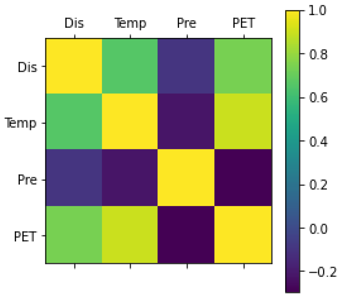
Table 2 shows the correlation between discharge, temperature, precipitation, and evapotranspiration. Discharge has the best correlation with evapotranspiration and a negative correlation with temperature. The temperature has a negative correlation with all three parameters. Precipitation has the best correlation with evapotranspiration which is also shown in
Figure 3.
2.2. Morphological Data Preprocessing
A vector and raster version of the Maipo basin is used to perform geospatial analysis and a data description is given in
Table 3. Hydro-basin of the Maipo catchment has been extracted from the gridded HydroSHEDS (Hydrosheds.org) as a vectorized polygon. For extracting elevation masks of the basin SRTM-DEMs raster data is used which is created using bi-static radar interferometry with a resolution of 30m. SRTM is created on a near-global scale between 56°S and 60°N, using C-band and X-band radar frequencies by the National Aeronautics and Space Administration (NASA), and German Aerospace Center (DLR).
The glacier outlines are taken from the Randolph Glacier Inventory ( RGIv6) [
33], with the position being Chilean glaciers, between-18 and-56 degrees, and latitude at release date 2018-07-24. In the Maipo River Basin, the non-gap filled DEM shows a veritably good content, except for many small glaciers, which weren't included (e.g., Morado Glacier) face hypsometry for each glacier is deduced from cutting the outlines with Digital Elevation Models ( DEMs). Ice consistency distribution of all glaciers of the Maipo basin is downloaded from the ETH Zurich exploration collection website and a Civilians routine is followed to achieve the hypsometry of the glacier.
Figure 4 represents the Maipo receptacle with its sub-basin, which is created for concentrating individual sub-basin to compare the glacier model for better output results. Figure showing the elevation of the glacier with elevation from 2500m to 6500 m amsl (above mean ocean level) and ice consistency with maximum 355m.
An overview of the different Maipo basins is outlined in
Table 5. Olivares basin has 12 glaciers consisting of 79.99
of area, 5925m maximum elevation, 3422 m mean elevation, and with max 326.84m ice thickness. The Colorado basin has 16 glaciers covering a 67.07
area, 6334 m of maximum elevation, and 2955 m mean elevation. The ice thickness is 293.70 m in the Colorado basin glaciers. Yeso basin has only 6 glaciers covering 67.05
which means the Yeso basin has the maximum area ratio as compared to other basin glaciers.
The maximum and mean elevation is 5904 m, and 3567 m, and the ice thickness is 219.04 m of the Yeso basin. The Volcan basin has 13 glaciers consisting of 70.62 of area, which is the second most glacierized area in the Maipo basin after the Olivares basin. The maximum and mean elevation is 5676 m, and 3367 m and ice thickness is 245.67m of Volcan basin. The Upper Maipo basin has 18 glaciers covering 59.22 of the area and maximum, mean elevation of 5404 m, 3319 m, and ice thickness of 271.17 m.
2.3. mHM (mesoscale hydrological model)
The mesoscale Hydrologic Model (mHM,
https://mhm-ufz.org) is a spatially explicit, grid-based hydrologic model. It is designed specifically to provide distributed predictions of various hydrologic variables such as runoff, evapotranspiration, soil moisture, and discharge along rivers. The model simulates the following processes: canopy interception, snow accumulation and melting, soil moisture dynamics, infiltration, surface runoff, evapotranspiration, subsurface storage, and discharge generation, deep percolation and baseflow, discharge attenuation, and flood routing.
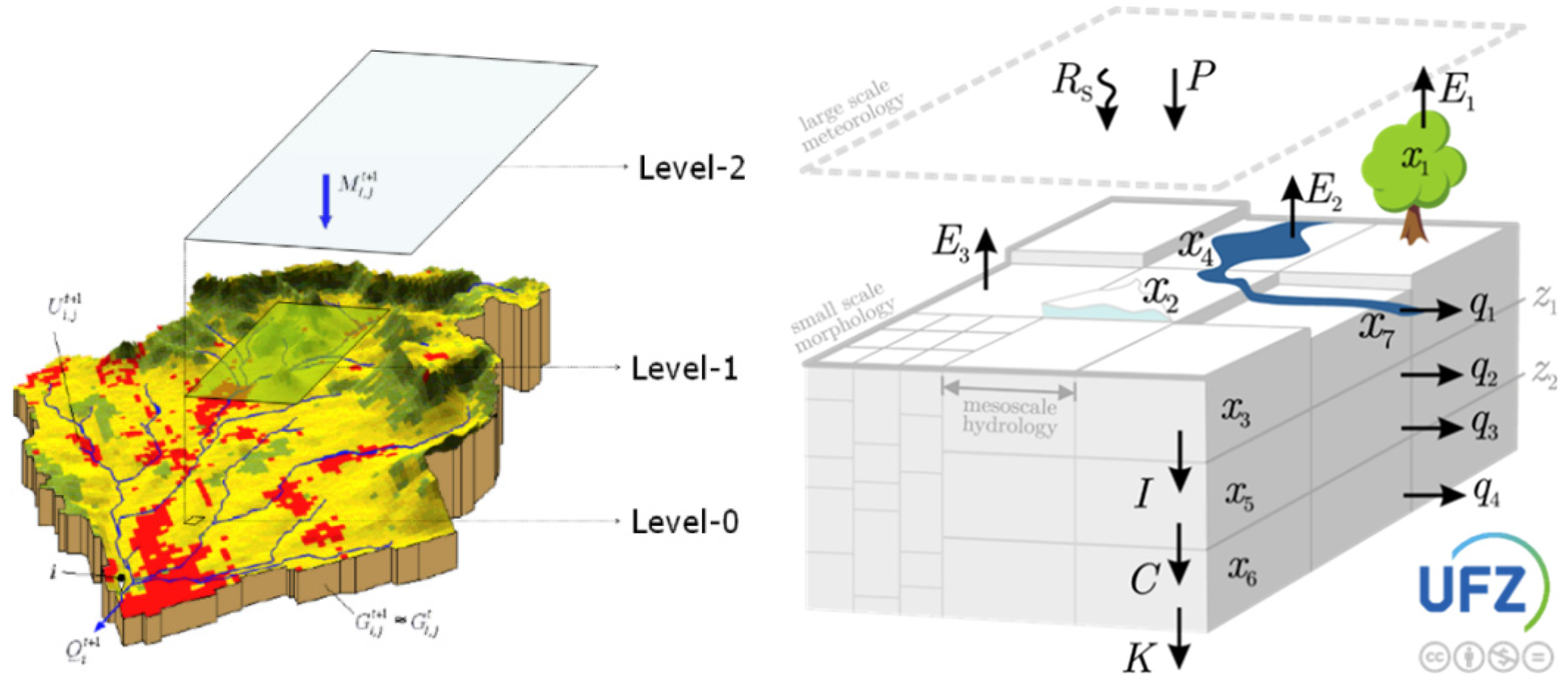
A mesoscale view of the hydrological cycle spans several orders of magnitude and consists of three levels (mHM levels), differencing them to better capture the spatial variability of variables and states.
Level-0: Spatial discretization suitable for representing the main terrain features, various soil characteristics (photos), the land cover, and the cell sizes is denoted by L0.
Level-1: Spatial discretization is used to describe dominant hydrological processes at the mesoscale and geological formations of the basin. This level's cell size is denoted by L1.
Level-2: Spatial discretization suitable to describe the variability of the meteorological forcing at the mesoscale, for example, the formation of convective precipitation. The cell size at this level is denoted by L2.
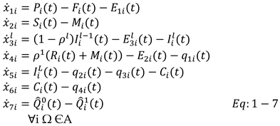
A mesoscale basin is a natural system composed of very heterogeneous materials with fuzzy boundary conditions. It is quite difficult to justify the continuity assumption of the input variables because most of the spatial heterogeneity of a basin can be explained by discrete attributes, such as soil texture, land cover, and geological formations. Therefore, a system of ordinary differential equations ODEs [
35] was adopted to describe the evolution of state variables at a given cell i within the domain Ω. This system of ODE:
Where,
| Inputs |
Description |
| P |
Daily precipitation depth, mm d−1
|
| T |
Daily mean air temperature, °C |
| Ep |
Daily potential evapotranspiration (PET), mm d−1
|
| Outputs |
Description |
|
Simulated discharge entering the river stretch at cell i, m3 s−1
|
|
Simulated discharge leaving the river stretch at cell i, m3 s−1
|
| Fluxes |
Description |
| S |
Snow precipitation depth, mm d−1
|
| R |
Rain precipitation depth, mm d−1
|
| M |
Melting snow depth, mm d−1
|
| Ep |
Potential evapotranspiration, mm d−1
|
| F |
Throughfall, mm d−1
|
|
E1
|
Actual evaporation intensity from the canopy, mm d−1
|
|
E2
|
Actual evapotranspiration intensity, mm d−1
|
|
E3
|
Actual evaporation from free-water bodies, mm d−1
|
| I |
Recharge |
| C |
Percolation, mm d−1
|
|
q1
|
Surface runoff from impervious areas, mm d−1
|
|
q2
|
Fast interflow, mm d−1
|
|
q3
|
Slow interflow, mm d−1
|
|
q4
|
Baseflow, mm d−1
|
| Indices |
Description |
| l |
ndex denoting a root zone horizon, /=1, L (say L= 3), in the first layer, 0 ≤ z ≤ z1
|
| t |
ime index for each Δr interval |
| ρl |
verall influx fraction accounting for the impervious cover within a cell |
To run mHM, we need several datasets such as meteorological, morphological variables, land cover, and gauging station information. All the meteorological variables are downloaded in NetCDF format and have hard-coded names such as 'tavg' for average temperature, 'pre' for precipitation, and 'pet' for evapotranspiration. There is an additional file called header.txt in every meteorological data file, and the easting and northing coordinates of the lower left corner should correspond to your catchment's morphological data. To maintain consistency in data, NODATA (-9999) value is specified in the header file. In addition, input mHM needs a latlon.nc file that specifies every grid cell's geographical location in WGS84 coordinates. The input for mHM also requires a latlon.nc file specifying the geographical location of each grid cell in WGS84 coordinates. Each resolution of the hydrological simulation at level-1 has to be adjusted. There are several morphological input datasets needed for MHM, and all of them must be provided in ArcGIS ASCII format, which stores the above header data and the actual data as plain text. Some raster files need to be supplemented with look-up tables that provide additional information. The required datasets and their corresponding filenames are given in
Table 8:
Figure 6 illustrates the workflow of the mHM model, a mHM setup is developed in Fortran 90 language and Linux system is used to run the model. Maipo basin including the meteorological forcing files and morphological files are prepared by UFZ Leipzig and used in this study. An mHM compilation file is required to run the mHM model for new applications and mhm.nml(namelist file) from the default model is used. After setting all the parameters for the Maipo basin and changing the name of the file as per
Table 8, the model is run as daily output. For post-processing the output result, python is used for plotting and visualization. All the mHM model files including input and output results available and shown in
Table 21 Digital Appendix.
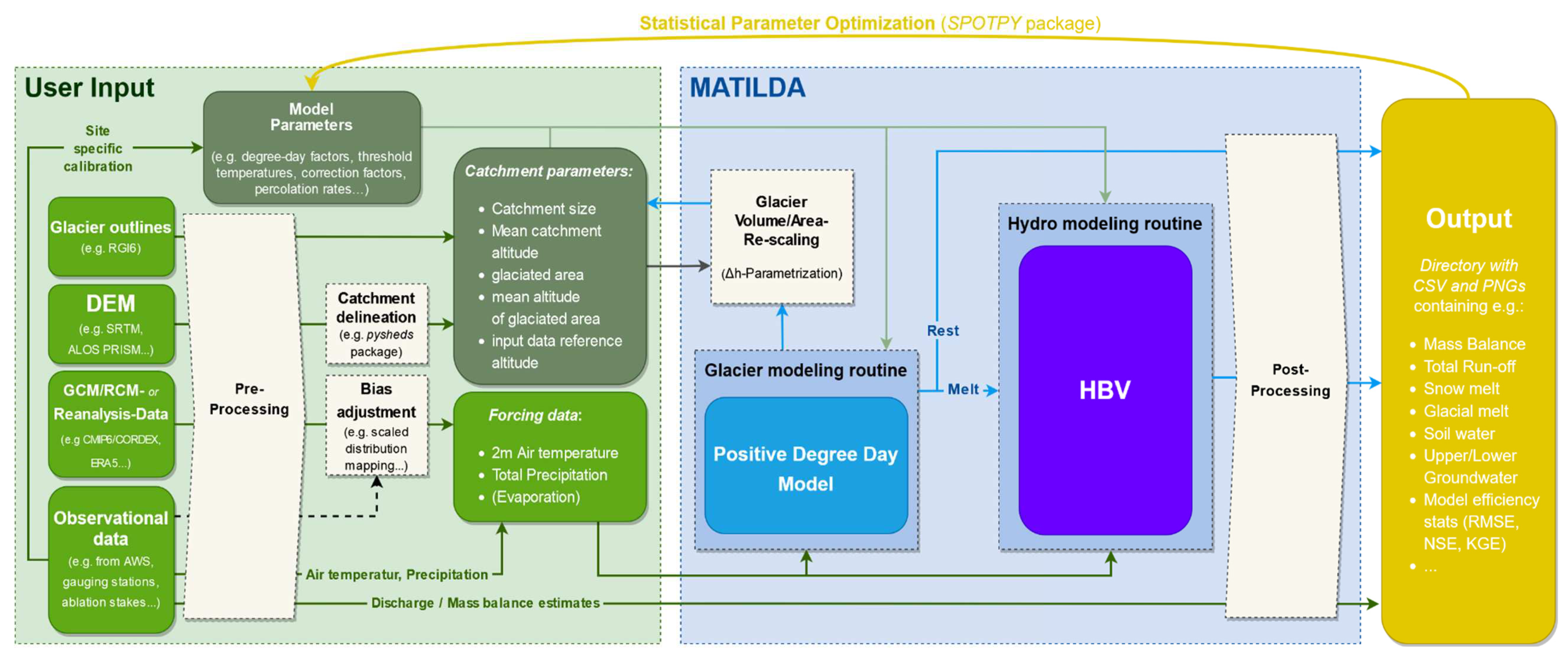
2.4. MATILDA – (Modeling Water Resources in Glacierized Catchments) MATILDA - Modeling Water Resources in Glacierized Catchments (https://github.com/ cryocoolers/matilda) model aims to provide an open-source tool that allows users to assess the characteristics of small and medium-sized glacierized catchments, as well as estimate future water resources based on scenarios of climate change. To compute glacial melt, the MATILDA framework combines a simple positive degree-day routine (DDM) with the hydrological bucket model HBV [36].
Figure 7 illustrates the workflow of the MATILDA model, in the first part, input data is preprocessed to use in the pypdd tool model and HBV model. To calculate glacial melt using a positive degree-day method, MATILDA employs a modified version of the pypdd tool. It also modifies HBV from the Lumped Hydrological Models Playground (LHMP). The output includes numerous displays of the input and output data as well as the modeled time series for various water balance components, basic statistics for these variables, and a choice of model efficiency coefficients (e.g., NSE, KGE
2.4.1. Pypdd
The Pypdd model [
37] simulates glacier surface mass balance using a positive degree-day model in Python. A simple model is provided here that computes glacier accumulation and melt based on near-surface air temperatures and precipitation records. PDD is a method developed by Reeh [
38] based on an empirical relationship between surface melt and temperature. During the model simulation, a normal distribution of temperature is assumed around the mean, as well as the possibility of melted snow and ice deposited on the surface of glaciers being re-frozen. Surface melt is commonly parameterized using the positive degree-day model for its simplicity [
39]. A melting rate proportional to the number of positive degrees-days, which is equal to the integral of the temperature (T) over a time interval(A):
The difference between snowfall and rain is determined by a threshold temperature, the threshold temperature of rain is calculated as
Where T (snow) is the temperature below which all precipitation is solid and T (diff) is the difference between the T (snow) and temperature above which all precipitation is liquid. Between T (snow) and T (diff) fractions of liquid and solid precipitation change linearly (°C). The ice melt factor is calculated as
CFMAX (ice) is the ice melt rate (mm/day per K above freezing point) and CFMAX (rel) is the constant factor to calculate the snow melt rate from CFMAX(snow). Precipitation is separated into liquid and solid fractions based on linear transitions between threshold temperatures.
Where T_reduce is calculated to use as a snow fraction by using threshold temperature and T (snow) and air temperature of the glacier (T2). Following that, snow melt is calculated by multiplying snow fraction by total precipitation (RRR). Rain results from the difference between precipitation and snow. Calculation of the melt rate is based on snow precipitation and positive degree day sums, and calculation of snowmelt is based on the number of positive degree days and attribute CFMAX (snow). If all the snow has melted and some energy remains (PDD), the ice melt is calculated using CFMAX (ice).
and, ice melt is proportional to excess snow melt.
Where Snow_melt is calculated by taking the minima of Snow and Pot (snow_melt). Accumulation, snow, ice melt, and runoff rate from the glaciers are calculated by using the Degree Day Model [
37]. Total melt is calculated by adding snow melt and ice melt.
The total runoff rate is calculated as the difference between the total melt and fraction of meltwater that refreeze in the snowpack and the fraction of ice melt refreezing.
A list of parameters used as input in the MATILDA model is shown in Table 9. Depending on the catchment, the parameter ranges are further constrained based on available information. An evapotranspiration correction factor is set to be 0 as evapotranspiration data is available from the mHM results, if in case evapotranspiration data is not available Oudin formula calculates evapotranspiration values. In this analysis, linear lapse rates are used to scale the forcing data to the mean glacier elevation and the mean catchment elevation, respectively.
Para-
meters
|
Description |
Range |
Unit |
| lr_temp |
Lapse rate of air temperature |
[-0.01, -0.003] |
(K/m) |
| lr_prec |
Lapse rate of precipitation |
[0, 0.002] |
(mm/m) |
| BETA |
The parameter that determines the relative contribution to runoff from rain or snowmelt |
[1, 6] |
|
| CET |
Evaporation correction factor |
[0, 0.3] |
|
| FC |
Maximum soil moisture storage |
[50, 500] |
|
| K0 |
Recession coefficient for surface soil box (upper part of SUZ) |
[0.01, 0.4] |
|
| K1 |
Recession coefficient for upper groundwater box (the main part of SUZ) |
[0.01, 0.4] |
|
| K2 |
Recession coefficient for lower groundwater box (whole SLZ) |
[0.001, 0.15] |
|
| LP |
The threshold for reduction of evaporation (SM/FC) |
[0.3, 1] |
|
| MAXBAS |
Routing parameter, order of Butterworth filter |
[2, 7] |
|
| PERC |
Percolation from soil to upper groundwater box |
[0, 3] |
|
| UZL |
Threshold parameter for groundwater boxes runoff |
[0, 500] |
(mm) |
| PCORR |
Precipitation (input sum) correction factor |
[0.5, 2] |
|
| TT_snow |
Temperature below which all precipitation is solid. Between TT_snow and TT_rain fractions of liquid and solid precipitation change linearly |
[-1.5, 2.5] |
(°C). |
| TT_diff |
Difference of TT_snow and temperature above which all precipitation is liquid (TT_rain). |
[0.2, 4] |
(°K) |
| CFMAX_ice |
Ice melt rate (mm/day per K above freezing point). |
[1.2, 12] |
|
| CFMAX_rel |
Factor to calculate snow melt rate from CFMAX_ice |
[1.2, 2.5] |
|
| SFCF |
Snowfall Correction Factor |
[0.4, 1] |
|
| CWH |
Fraction (portion) of meltwater and rainfall which retains in the snowpack (water holding capacity). |
[0, 0.2] |
|
| AG |
Calibration parameter for glacier storage-release scheme. High values result in a small reservoir and instant release. Low values extend storage and delay release. |
[0, 1] |
|
| RFS |
Fraction of meltwater that refreezes in the snowpack. |
[0.05, 0.25] |
|
| pfilter |
Threshold above which precipitation values are elevation scaled using lr_prec. This addresses the common issue of reanalysis data to overestimate the frequency of low precipitation events. Handle with care! Should be fixed depending on the input data before parameter optimization. |
[0, 0.5] |
|
2.4.2. Glacier retreat model
To calculate glacier area evolution in the study period, Huss and Hock 2015's [
26] introduce ∆h parameterization which is included in the degree-day routine (DDM) routine. As a data frame, the routine needs the initial glacier profile containing the spatial distribution of ice over elevation bands at the beginning of the study period. This ∆h parametrization routine is based on the workflow outlined in Seibert et al. [
40]. In response to a change in mass balance, ∆h-parameterization describes the spatial distribution of glacier surface elevation variation. It is an empirical approximation method to characterize the glacier retreat at the scale of a particular glacier and is subject to uncertainty and several limitations. Huss et al. [
41] originally developed this approach for periods dominated by negative mass balances and glacier retreat. This is a more efficient state-of-the-art alternative to more complex glacier evolution models. For glacier mass changes to be translated into glacier area changes, a single-valued relationship needs to be established. In the model, this relationship is represented by a lookup table, which provides glacier areas for the different elevation zones based on a specific glacier mass value.
A glacier's volume can be calculated by integrating its initial glacier profile, which is a graphical representation of the area and thickness of a glacier (measured in mm water equivalent).
Where,
M is the total glacier mass in
mm water equivalent relative to the entire catchment area, and for each elevation band
i,
the area (expressed as a proportion of the catchment area) and water equivalent
in mm. The normalized elevation
for each elevation band is derived from the absolute elevation of the corresponding elevation band i, as well as the maximum and minimum elevations of the glacier,
and
.
For each of the normalized elevations, the normalized water equivalent change is calculated using the following function (Huss et al., 2010).
where
is the normalized (dimensionless) ice thickness change of elevation band
i and
a, b and
c, and
γ are empirical coefficients. These empirical coefficients are based on the glacier size class. If the glacier area is greater than 20
then a = -0.05, b = 0.19, c = 0.01, and y = 4 are chosen by Huss et al. [
41]. Glacier volume balance change
is computed by using a scaling factor
(mm) which scales the dimensionless
, and the glacier mass with normalized water equivalents change for each of the elevation bands.
For each elevation band, the new water equivalent
is computed starting from the user-specified initial glacier thickness profile for t=0 as
In this equation,
represents the water equivalent of elevation band i after reducing the glacier mass t times by
. After the new water equivalent values for each elevation zone have been computed, the glacier area is updated accordingly. It is common for glaciers at elevations to have uneven distributions of ice, with thinner ice layers along their edges. This uneven distribution results in a reduction in area, so a simplified representation of glacier geometry is used to scale the area within certain elevation bands (Eq. 7) based on Bahr et al. [
42] and Huss and Hock [
26], which also applies relationship between glacier width and glacier thickness:
A reduction in glacier area over elevation was observed because of the combination of ∆h parameterization (Eqs (16) through (21)) with glacier width scaling (Eq. 22). As a result of this, the glacier area and glacier mass relationship is stored in a lookup table in steps of 1 percent of the initial glacier mass.
2.4.3. Matilda Data Preparation and Initializations
ArcGIS tool is used to extract spatial information from the Maipo catchment and glaciers by using geo-processing tools for analyzing, editing, and converting data. For creating a Glacier profile of a glacier, area, and water equivalent per elevation band are required. The following steps are followed to create the input file for the MATILDA model.
Firstly, several glaciers are selected for individual basins which are available as ice thickness raster data, and then all non-available number (NAN) of rater data is removed and merged into one raster file. Each basin raster is extracted individually and merged into one by using SRTM raster data and vectorized polygon. Contour is created by using merged glacier raster data with 10m of elevation band and then zonal statistics as the table is created by using a contour vectorized polygon of the glacier and ice thickness data.
To run a Matilda model, several required input variables are prepared by using CAMEL-CL data sources. Input variables such as air temperature (°C), total precipitation (mm), and (if available) evapotranspiration data (mm). To calibrate the model, runoff observations are used, units of runoff change from
to mm/day, and all data sets are prepared as daily resolutions. Matilda offers glacier modeling as an optional option to include the
h parameterization from Huss and Hock [
26] within the DDM routine and to calculate glacier area evolution during the study period. To conduct the routine, an initial glacier profile is created, which contains the spatial distribution of ice over elevation bands at the beginning of the study period.
Elevation - elevation of each band with a resolution of 10 m.
Area - an area of each band as a fraction of the total glacier area
WE - ice thickness in mm w.e.
EleZone - combined bands over 100-200 m.
A base contour is used with a 10m resolution starting with the lowest elevation of the glacier. The glacier ice thickness raster file is used to create the zonal statistics for all the bands available for the glaciers. The area is extracted from the zonal statistics table for each elevation band and the unit is changed from to . The thickness of a glacier is converted to grams of water equivalents (mm) by applying an ice density of 906 kilograms. A mass balance term is expressed as water equivalents (w.e.) to allow comparisons to be made between different glaciers. In a snow or ice melting scenario, the water equivalent represents the volume of water that is produced by the glacier.
The MATILDA package comprises four different modules such as parameter setup, data preprocessing, simulation core, and post-processing. A complete workflow can be used via the MATILDA_simulation function or through the individual modules as well. To use the MATILDA_simulation function, the following steps are followed to accomplish the run.
After downloading and installing all the dependencies of MATILDA, spin-up and simulation periods are defined with one year of spin-up. Catchment properties such as catchment area, glacierized area, average elevation, and average glacier elevation are specified. The output frequency is defined as daily. (Option: daily, weekly, monthly, or yearly). Using the MATILDA_parameter function parameters are specified and if no parameters are specified, default values are applied. MATILDA_preproc function is run to use the data preprocessing. MATILDA_submodules function is used to run the actual simulation. MATILDA_plots function is used to plot the runoff, meteorological parameters, and HBV output variables using.
For running the MATILDA model, the MATILDA package, dependencies and other following python library is installed (Xarray, numpy, pandas, matplotlib, scipy, datetime, hydroeval, HydroErr, and Plotly).
Figure 8 shows the workflow of the mHM and MATILDA melt model. For preparing the MATILDA melt file, a text file is prepared from the output result of the MATILDA on hourly bases to run into the mHM model. All the model files including input and output results available as shown in
Table 21 Digital Appendix
. 2.4.4. Calibration and Criteria
To evaluate the calibration parameters and to analyze results in the following chapters, a variety of statistical measures is employed. A summary of the measures used in this thesis can be found here, whereas Krause et al. [
43] provide a more comprehensive discussion of each measure and alternative measures. The parameters of runoff models are traditionally calculated by calibrating against observed runoff and not by verifying internal model variables. Because of this, there may be a chance of compensating for errors [
44], and it may well be the case that the model performs well concerning runoff, even with an incorrect snow or ice distribution.
Many studies use the coefficient of determination for multivariate scenarios, or r^2 and it provides a dimensionless value between 0 and 1, where 1 represents the optimum performance of the model. And can be calculated as
where:
= model discharge at time t
= is the observed discharge at time t= average runoff during the calculation period
n = number of days in the calculation period
A widely used specification for the NSE criterion of runoff developed by Nash and Sutcliffe [
45] is widely used in the calibration and evaluation of rainfall-runoff models. Its value ranges from -∞ to 1, if the simulated runoff value is greater than zero, the simulated runoff represents a good observable representation of actual runoff variations better than the observed long-term average.
The Root Mean Square Error (RMSE) reveals the mean difference between modeled
and observed
discharge:
The advantage of using this method is that it preserves the units of the original data, so measurements can be compared to see the magnitude of errors, not just the model's performance. RMSE values approaching zero represent a better agreement between observations and predictions, but, likewise r^2, it has a limitation due to its large bias toward outliers.
The model execution of the Matilda applications is here evaluated with the modified Kling-Gupta Efficiency (KGE) [
46]:
where,
r = Pearson Correlation Coefficient
Where
is the mean of observed values,
is the mean of simulated values,
is the standard deviation of simulated values and
is the standard deviation of observed values. KGE = 1 means an ideal match between simulated and observed values, and KGE ≈ -0.41 indicates the model simulation is as accurate as the observed mean (Knoben et al., 2019. For analysis mHM and Matilda model KGE, NSE, and RMSE model efficiency coefficients are employed by using the “HydroErr” library [
47].
4. Discussion
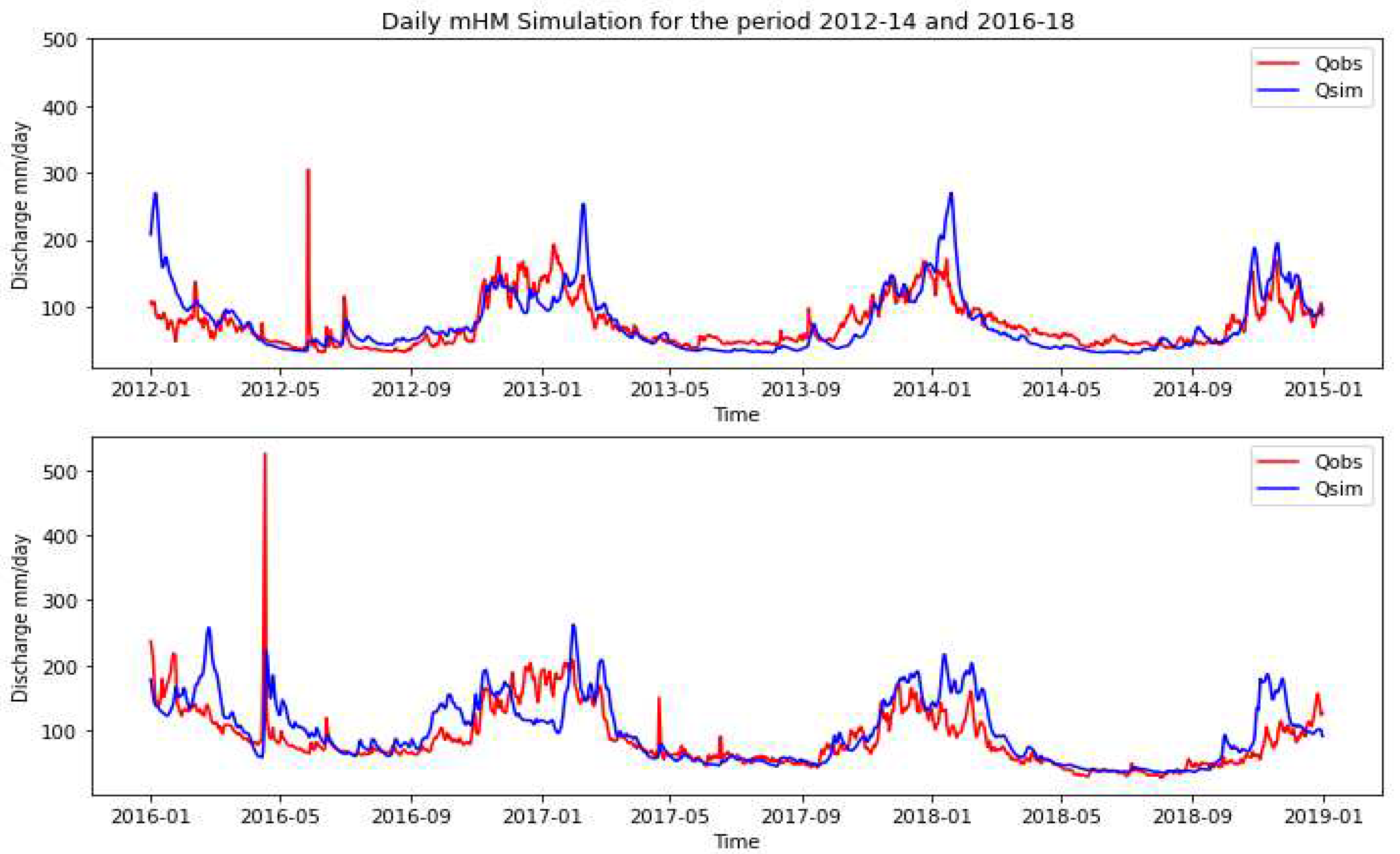
For the periods 2012-2014 and 2016-2018, the calibration of the mHM model for NSE is 0.40 and 0.15, whereas for MATILDA have 0.25 and 0.20. mHM is showing a good result for the first period and MATILDA has good results with NSE values. For KGE, observed and mHM simulation of stream flow is 0.70 and 0.53 for the period 2011-2014 and 2015-2018. Since the KGE values for the MATILDA model are 0.41 and 0.44 for the period 2011-2014, KGE values for mHM represent better results than those of MATILDA.
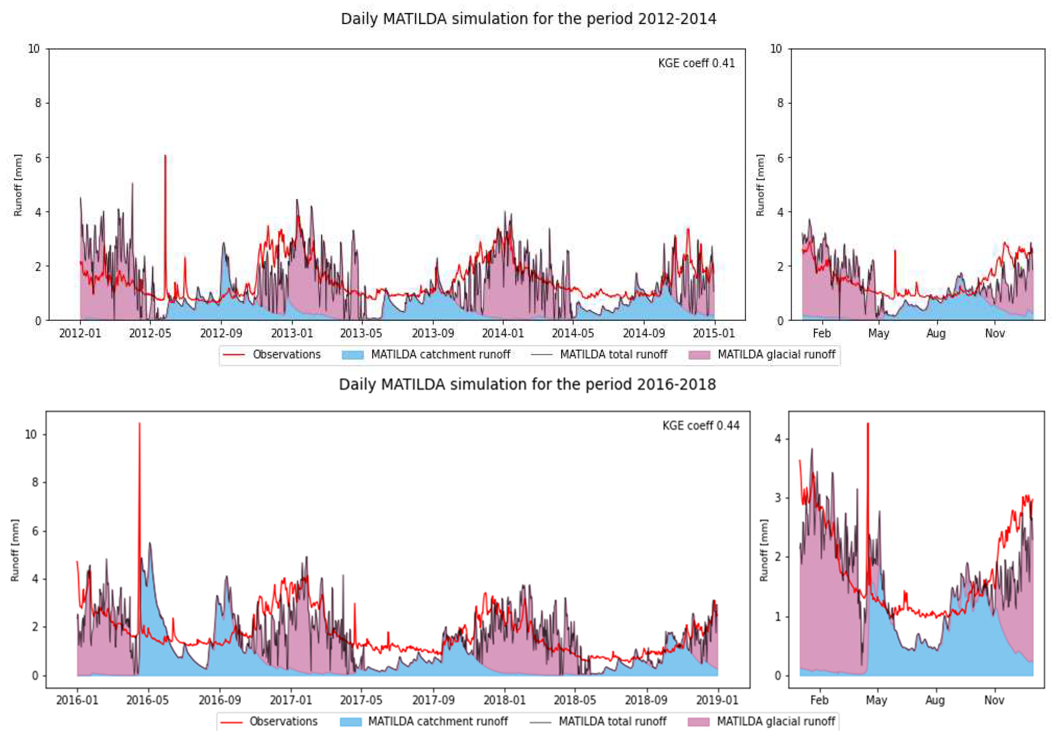
The daily mean streamflow (m^3 s^(-1)) calculated by mHM is less than the mean observed streamflow in both periods 2012-2014 and 2016-2018. In the MATILDA model mean runoff(mm/day) calculated is less than the observed mean flow, so both models have not reached the observed mean values (tables 10 and 13). mHM and MATILDA both models couldn’t reach the maximum of the observed streamflow on any day of the simulation periods. In the summer and winter seasons mHM produces more average discharge than the observed average discharge. In the MATILDA model, in every season observed mean runoff is more than the simulated runoff. MATILDA produced well during the summer season, except early in 2012 with high runoff due to Chilean summer. However, after late spring, there was a sudden decrease in simulation.
For the entire Maipo basin, the Matilda model is giving an average result. Mostly, in winter when there is no glacier runoff the model is poorly performed, seen in
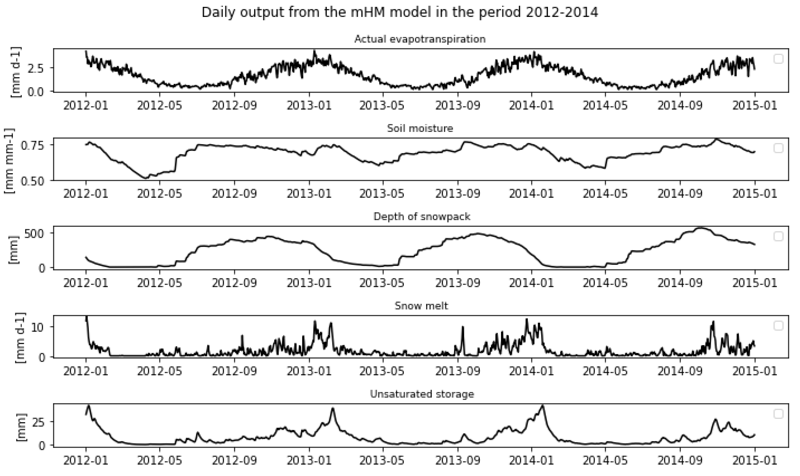
Figure 11. The catchment runoff contribution without glaciers varied by 31% during 2012-2014, but the contribution with glaciers was more than twice as large as without glaciers. The glacier melt is more in 2016-18 as compared to 2012-14 but the glacier area reduction percentage is not much different because it is assumed in the model that the initial glacier profile for both periods is the same, which is not in the real scenario. Individual sub-basin analysis was also performed with the mHM model and among all the basins, the Colorado and Yeso sub-basins have the highest and same KGE value of 0.36 (table 18) and, whereas Olivares and Upper Maipo basins have the lowest. The calibration result of mHM shows that the model is working very well even without having a glacier module, on the other hand, MATILDA is showing average results. Overall mHM model perform well especially in 2015-18 even though there are some missing values in observed data.
4.1. Limitations and Outlooks
This research study was carried out by using two datasets ERA5 and CAMELS-CL for mHM and MATILDA models. The mHM model uses grid-based datasets which are not available in the CAMELS dataset, whereas the MATILDA model can run with the ERA5 dataset by aggregating. The MATILDA model is subject to some uncertainty largely because of input parameterizations and is not suitable for a big catchment. Matilda's main drawback is that it uses HBV, which always requires parameter calibration, whereas mHM can always be applied. Some parameters are difficult to calibrate since they affect the calibration objectives indirectly, and can be readily compensated for by other more dominant parameters [
48]. In the Maipo catchment, there are permafrost and rock glaciers which have not been modeled in the present study due to a lack of knowledge in the study case area. Because of the significantly smaller catchment area and the high data quality of the nearby glacier station, the results can be rated as satisfactory and generally better.
For further research, it is more appropriate to use the ERA5 dataset for both models so that better comparisons can be made. Model mHM and MATILDA both need 3 forcing data such as precipitation, temperature, and evapotranspiration and perform well with a degree day approach at the cost of limited data requirement, although they are not reliable in some cases when the radiation is too high at the top and a large portion of the melt will evaporate. The glacier can also melt at low temperatures because of the sunlight. Moreover, the algorithm used for glacier mass balance and retreat can be further improved by including solar radiation and topographic factors in the degree-day factors. In addition, glacier mass balance components can be modeled with an energy balance approach. Although, it is more accurate to use physically-based glacier models to estimate future glacier dynamics and the redistribution of glaciers and snow if the climatic and hydrological systems are not stable [
6] (Hock, 2005). MATILDA as a lumped model did not work well during the phase transition from Autumn to Winter season, in this case, a fully distributed model (mHM) can improve the streamflow by adding glacier melt distribution over the glacier elevation bands including evident slope and elevation zone according to the aspect classes. Once enough input and validation data are available, the physical models can be developed and used in glacier modeling.
5. Conclusions
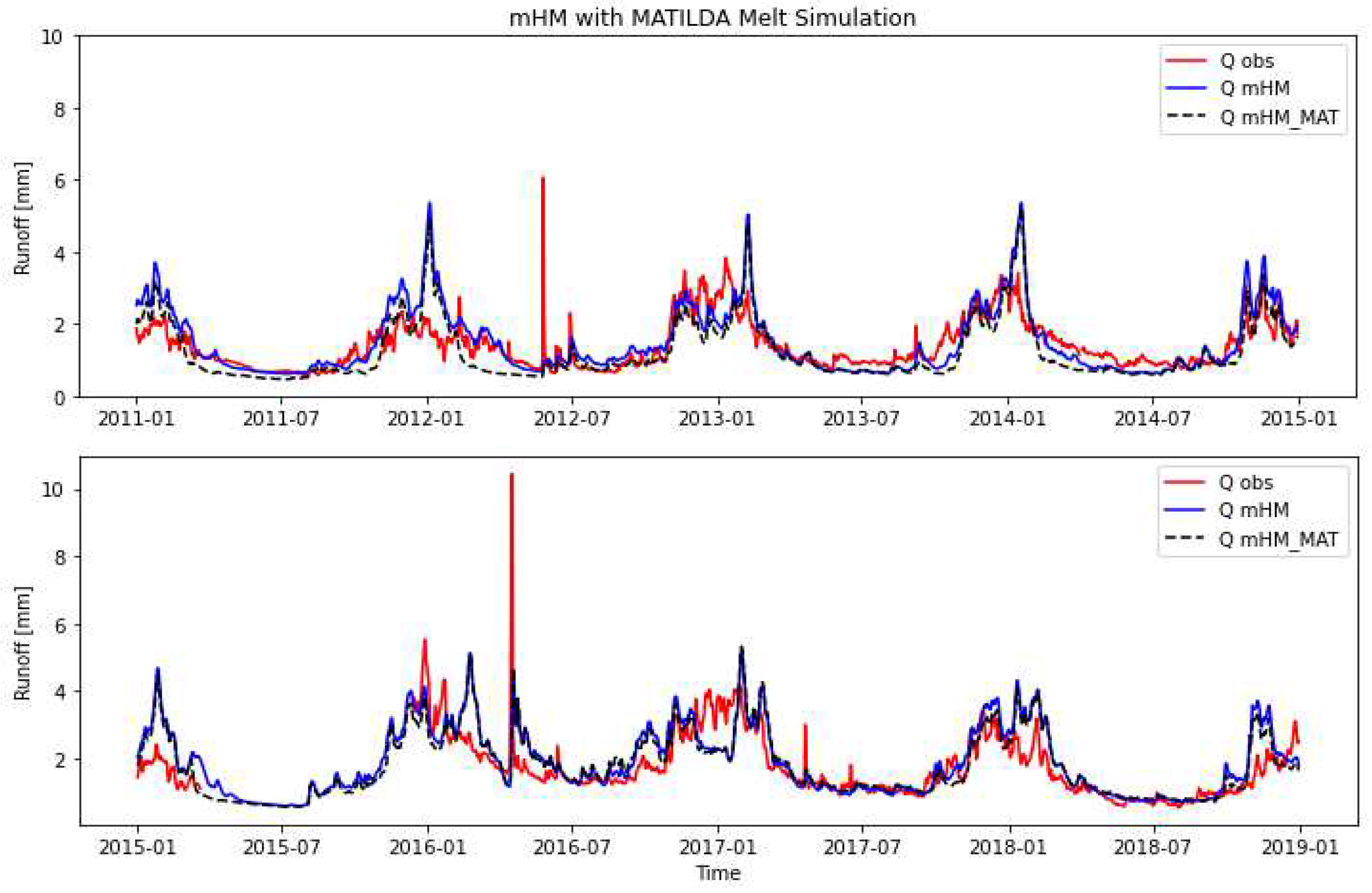
Generally, mHM mimics acceptably seasonal flow dynamics as compared to MATILDA, as MATILDA has only a glacier-distributed unit, while mHM is a fully spatially distributed model. In the initial days, MATILDA performance was poor due to the overestimation of the input parameterization. The initial storage condition, glacier area, and elevation distribution are possibly underestimated when Matilda parameterization is performed, which results in some of the ablation period being lost because of the run bias and it is also possible due to less warm-up period. The Olivares basin has only 20% of the Maipo basin glacier with very high altitude and low temperature and provides very low glacier melt to overall glacier melt. Thus, the mHM with MATILDA Olivares melt model and the mHM without MATILDA Olivares melt models output result doesn’t have much difference. To use glacier melt from the MATILDA approach, the mHM melting component is replaced with the MATILDA melt by internalizing it into the mHM model. Model mHM with MATILDA melt performed well in 2015-18 as compared to 2011-15 with having r^2 values of 0.3721 and 0.2532 respectively. Whereas mHM have just 0.2532 and 0.2941. But surprisingly mHM_MAT performed poorly in the initial year of modeling.
To conclude, based on the results obtained, it is indicated that the mHM Model had a good performance to predict runoff and can be a potential monitoring tool for watershed management in a mountainous area. The MATILDA model was able to calculate the impact of glaciers during the summer and autumn seasons but in winter and spring, it performs poorly. The results from both model tools show variations in the results due to spatial resolution differences and their methodology. MATILDA has a glacier retreat routine that gives better result for the glacier characteristics such as ‘runoff from the glacier’ and ‘runoff without glacier’ and ‘glacier area’. The incorporation of MATILDA melt in a simple approach should be further developed in future research for the whole Maipo catchment, which includes glacier melt distribution in mHM models. The Glacier Modelling approach can be further improved by including solar radiation and Energy balance models, especially for high-altitude glacier regions. Analyzing the sensitivity of the parameters used to calibrate the model.
Table 21.
Digital Appendix model folder files details.
Table 21.
Digital Appendix model folder files details.
| |
|
mHM Model |
MATILDA Model |
mHM MATILDA Model |
| 1. |
Initial Model File: |
mHM Sources
(mhm-v5.11.1)Folder |
|
mHM Sources
(mhm-v5.11.1)Folder |
| |
|
Maipo Model
(5710001)Folder |
|
Maipo Sub-Basin Model
(5710001)Folder |
| 2. |
Input File: |
|
|
|
| |
Meteorological Data |
Precipitation(pre.nc) Temperature(tavg.nc) Evapotranspi(pet.nc) |
Forcing.csv
Glacier_profile.csv
Runoff_data.csv |
Precipitation(pre.nc) Temperature(tavg.nc) Evapotranspi(pet.nc)
Mat_melt.csv |
| |
Morphological Data |
Aspect.asc
Dem.asc
Facc.asc
Geology_class.asc
IDgauge.asc
Lc.asc
Slope.asc
Soil_class.asc |
Maipo_basin.shp
Maipo_basin.tif
Maipo_glacier.shp
Maipo_glacier.tif
Glacier_thickness.tif |
Maipo_basin.shp
Maipo_subbasin.shp
Maipo_basin.tif
Maipo_subbasin.tif
Maipo_glacier.shp
Maipo_glacier.tif
Glacier_thickness.tif |
| 3. |
Preprocessing Files |
Hypsometry.py
Resampling melt.py |
Input_data_pre.py
GIS_routine.py |
Input_data_pre.py
GIS_routine.py |
| 4. |
Post-processing files |
mHM_Plotting.py |
Matilda_Plotting.py |
mHM_Mat_Plotting.py |
| 6. |
Final Model Files |
mhm.nml |
matilda.py |
mhm.nml |
| |
|
|
|
|
| |
Flies Link |
https://github.com/ahmadmum/msc_thesis_glacier_modelling.git |
Figure 1.
A case study in Maipo Basin and the location of gauge, river, and lakes.
Figure 1.
A case study in Maipo Basin and the location of gauge, river, and lakes.
Figure 2.
Daily Meteorological Data (Discharge, Precipitation, Temperature, and Evapo.).
Figure 2.
Daily Meteorological Data (Discharge, Precipitation, Temperature, and Evapo.).
Figure 3.
Correlation Matrix.
Figure 3.
Correlation Matrix.
Figure 4.
Maipo Sub-Basin Glacier Elevation and Ice Thickness.
Figure 4.
Maipo Sub-Basin Glacier Elevation and Ice Thickness.
Figure 10.
mHM simulation (Qsim, blue) and observed stream flow (Qobs red).
Figure 10.
mHM simulation (Qsim, blue) and observed stream flow (Qobs red).
Figure 11.
mHM Model Output (Actual evapotranspiration, Soil moisture, Depth of snowpack, Snowmelt, and Unsaturated storage) for 2012-2014.
Figure 11.
mHM Model Output (Actual evapotranspiration, Soil moisture, Depth of snowpack, Snowmelt, and Unsaturated storage) for 2012-2014.
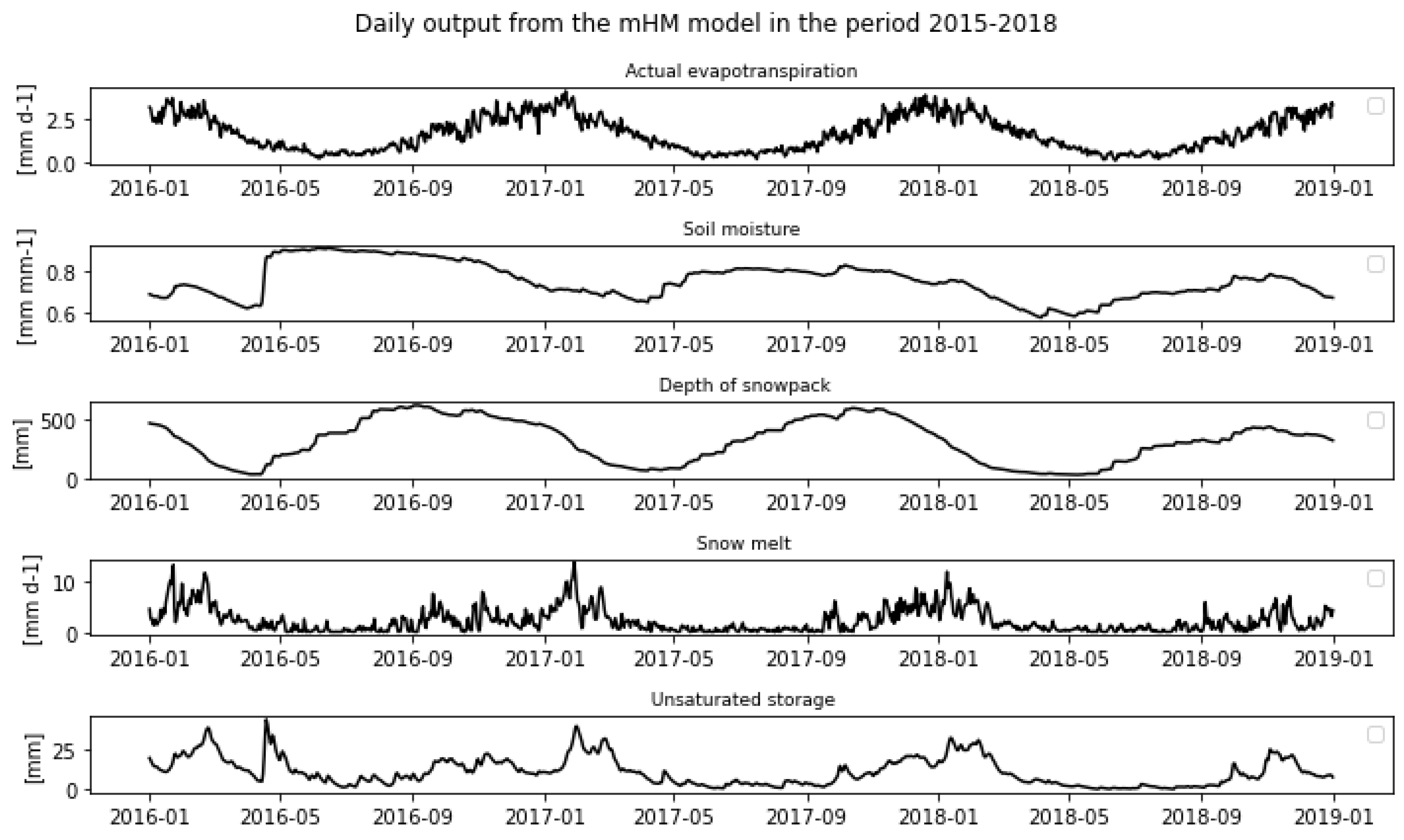
Figure 12.
mHM Model Output (Actual evapotranspiration, Soil moisture, Depth of snowpack, Snowmelt, and Unsaturated storage) for 2016-2018.
Figure 12.
mHM Model Output (Actual evapotranspiration, Soil moisture, Depth of snowpack, Snowmelt, and Unsaturated storage) for 2016-2018.
Figure 13.
MATILDA Runoff Simulation with observation from 2012-14 and 2016-18.
Figure 13.
MATILDA Runoff Simulation with observation from 2012-14 and 2016-18.
Figure 14.
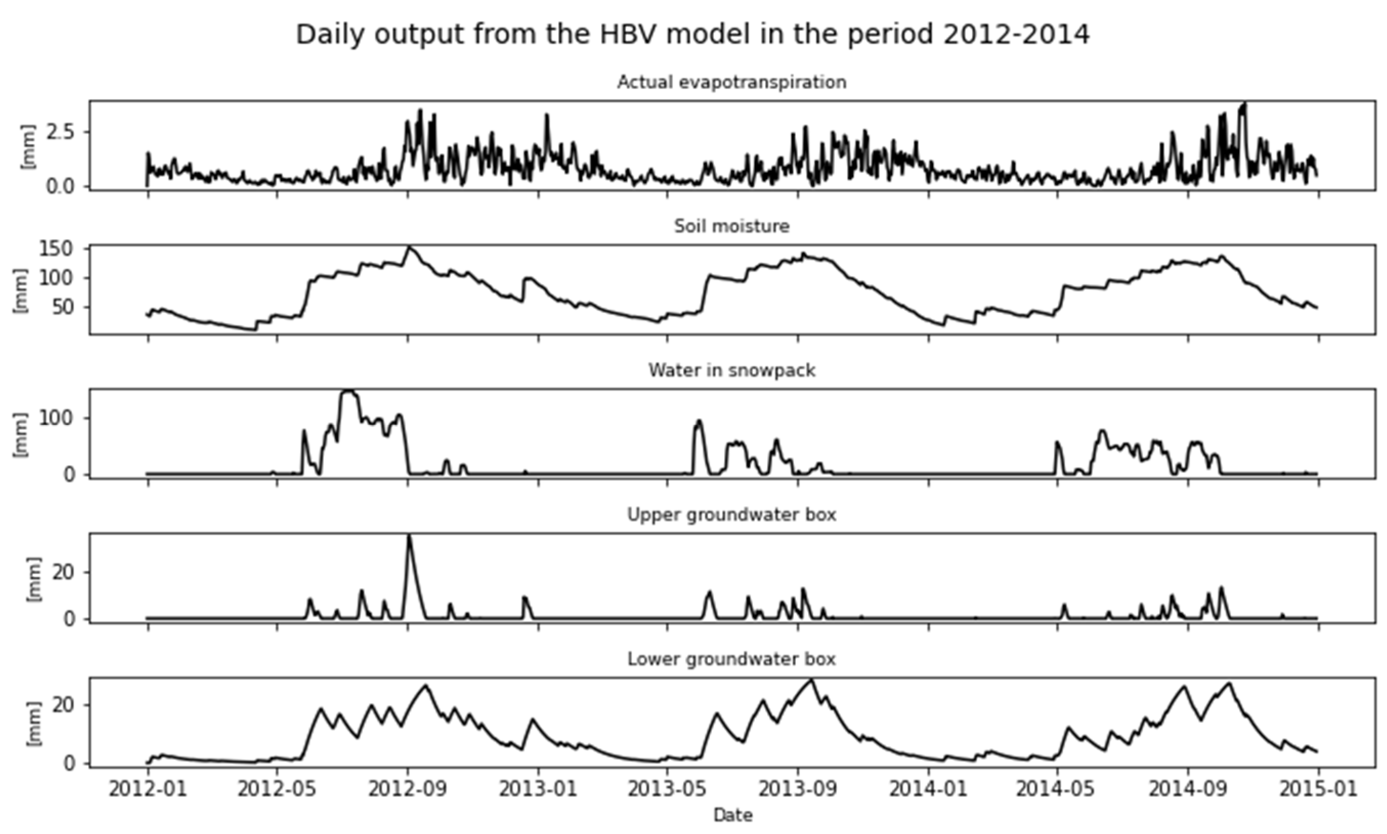
HBV Model Output (Actual evapotranspiration, Soil moisture, Water in the snowpack, Upper and Lower groundwater box) for 2012-2014
Figure 14.
HBV Model Output (Actual evapotranspiration, Soil moisture, Water in the snowpack, Upper and Lower groundwater box) for 2012-2014
Figure 15.
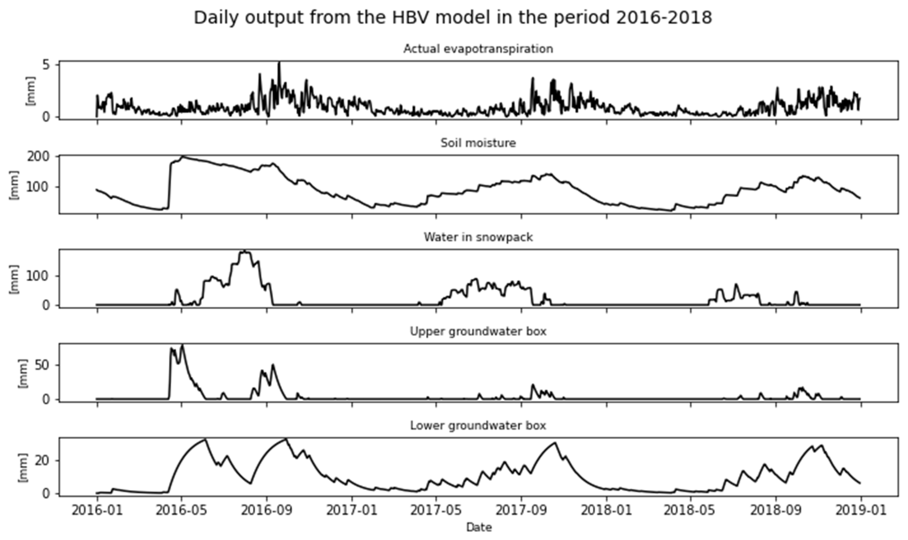
HBV Model Output (Actual evapotranspiration, Soil moisture, Water in snowpack, Upper and Lower groundwater box) for 2016-2018.
Figure 15.
HBV Model Output (Actual evapotranspiration, Soil moisture, Water in snowpack, Upper and Lower groundwater box) for 2016-2018.
Figure 17.
mHM, MATILDA, and mHM with MATILDA_Melt Observed Vs Simulation runoff.
Figure 17.
mHM, MATILDA, and mHM with MATILDA_Melt Observed Vs Simulation runoff.
Figure 18.
MATILDA Total melt of Olivares sub-basin.
Figure 18.
MATILDA Total melt of Olivares sub-basin.
Table 1.
Daily Meteorological Metadata from 2011-2018.
Table 1.
Daily Meteorological Metadata from 2011-2018.
| |
|
Preci(mm) |
Temp(C°) |
PET(mm) |
| Mean |
77.41 |
2.97 |
2.70 |
2.04 |
| Min |
26.3 |
0 |
-16.51 |
0.06 |
| Max |
526 |
104.30 |
16.58 |
5.43 |
| Std |
39.97 |
7.47 |
6.21 |
1.27 |
Table 2.
Daily Meteorological data correlation.
Table 2.
Daily Meteorological data correlation.
| |
Dis |
Temp |
Pre |
PET |
| Dis |
1.0 |
-0.09 |
0.65 |
0.73 |
| Pre |
0.65 |
-0.22 |
1.0 |
0.89 |
| Temp |
-0.09 |
1.0 |
-0.22 |
-0.29 |
| PET |
0.73 |
-0.29 |
0.89 |
1.0 |
Table 3.
Spatial Data Sets Used for Setting Up the mHM Model and MATILDA.
Table 3.
Spatial Data Sets Used for Setting Up the mHM Model and MATILDA.
| Sort |
Format |
Description |
Resolution |
Source |
| DEM |
Raster |
SRTM |
30m |
Tachikawa et al., 2011 |
| Basin |
Vector |
HydroBasin |
Polygon |
Lehner, B., Grill G. (2013) |
Glacier
Outlines |
Vector |
Glacier Outlines RGI v6.0 |
Polygon |
Pfeffer et al., 2014 |
Glacier
Profile |
Raster |
Glacier Ice thickness |
25m |
Farinotti D., M. Huss 2019 |
Table 4.
Characteristics of Maipo Sub-basin .
Table 4.
Characteristics of Maipo Sub-basin .
Basin
Name |
Lan &
Lon |
Area
|
Mean Elev(m) |
Max Elev(m) |
No. of Glaciers |
Glacier
|
Max. Ice Thickness |
| Olivares |
-33.49,-70.14 |
541.6 |
3690 |
6049 |
12 |
79.99 |
326.84 m |
| Colorado |
-33.49,-70.13 |
783.4 |
3737 |
6550 |
16 |
67.07 |
293.70 m |
| Yeso |
-33.80,-70.21 |
626.6 |
3567 |
5904 |
6 |
67.05 |
219.04 m |
| Volcan |
-33.81,-70.21 |
523.4 |
3367 |
5676 |
19 |
70.62 |
245.67 m |
| Upp. Maipo |
-33.98,-70.15 |
1035.5 |
3319 |
5404 |
18 |
59.22 |
271.17 m |
Table 5.
Equations 1-7 parameters with description.
Table 5.
Equations 1-7 parameters with description.
| States |
Description |
|
Depth of the canopy storage, mm |
|
Depth of the snowpack, mm |
|
Depth of soil moisture content in the root zone, mm |
|
Depth of impounded water in reservoirs, water bodies, or sealed areas, mm |
|
Depth of the water storage in the subsurface reservoir, mm |
|
Depth of the water storage in the groundwater reservoir, mm |
|
Depth of the water storage in the channel reservoir, mm |
Table 8.
Morphological data for mHM initialization.
Table 8.
Morphological data for mHM initialization.
| Description |
Raster, File name |
Sink filled Digital
Elevation Model |
dem.asc |
| Slope map |
slope.asc |
| Aspect Map |
aspect.asc |
| Flow Direction map |
fdir.asc |
| Flow Accumulation |
facc.asc |
| Gauge(s) position |
idgauges.asc, .txt |
| Soil map |
soil_class.asc, .txt |
| Hydrogeological |
geology_class.asc, .txt |
| Leaf Area Index |
LAI_class.asc, .txt |
| Land use map |
lc.asc |
Table 10.
Observed and mHM simulation Stream flow calibration results on a daily and the monthly basis from 1950 to 2020.
Table 10.
Observed and mHM simulation Stream flow calibration results on a daily and the monthly basis from 1950 to 2020.
| Calibration parameters |
Daily |
Monthly |
| |
Qobs/Qsim |
Qobs/Qsim |
|
0.26 |
0.30 |
| NSE |
0.70 |
-0.24 |
| KGE |
0.80 |
0.65 |
Table 11.
Observed and mHM simulation Stream flow calibration results daily from 2011-2014 and 2015-2018.
Table 11.
Observed and mHM simulation Stream flow calibration results daily from 2011-2014 and 2015-2018.
| Calibration parameters |
2011-2014 |
2015-2018 |
| |
Qobs |
Qsim |
|
0.007 |
-0.21 |
| NSE |
0.40 |
0.15 |
| KGE |
0.70 |
0.53 |
Table 12.
mHM Descriptive statistics for Daily streamflow ).
Table 12.
mHM Descriptive statistics for Daily streamflow ).
| |
2012-2014 |
2016-2018 |
| Mean |
70.61 |
62.53 |
88.69 |
87.16 |
| Min |
28.1 |
14.03 |
26.3 |
15.63 |
| Max |
305 |
265.91 |
526 |
258.11 |
| Std |
33.51 |
46.42 |
46.19 |
50.97 |
Table 13.
Descriptive statistics for Seasonal runoff () from 2012-2018.
Table 13.
Descriptive statistics for Seasonal runoff () from 2012-2018.
| |
Summer |
Autumn |
Winter |
Spring |
| |
Qobs |
Qsim |
Qobs |
Qsim |
Qobs |
Qsim |
Qobs |
Qsim |
| Mean |
125.88 |
130.95 |
49.61 |
42.62 |
65.87 |
57.52 |
81.73 |
89.76 |
| Min |
48.6 |
37.30 |
26.3 |
26.44 |
28.1 |
20.64 |
40.5 |
31.97 |
| Max |
237 |
265.91 |
119 |
96.51 |
526 |
214.90 |
175 |
191.85 |
| Std |
35.98 |
46.38 |
13.24 |
14.56 |
31.73 |
34.35 |
32.85 |
44.14 |
Table 14.
Descriptive statistics of mHM Model Output (Actual evapotranspiration, Soil moisture, Depth of snowpack, Snowmelt, and Unsaturated storage).
Table 14.
Descriptive statistics of mHM Model Output (Actual evapotranspiration, Soil moisture, Depth of snowpack, Snowmelt, and Unsaturated storage).
| |
Actual Evapotrans.
(mm/day) |
Soil moisture
(mm/mm) |
Depth of snowpack
(mm) |
Snow melt
(mm/day) |
Unsaturated storage
(mm) |
| Mean |
1.59 |
0.70 |
261.43 |
1.91 |
9.15 |
| Min |
0.003 |
0.51 |
0 |
0 |
0.037 |
| Max |
4.19 |
0.91 |
679.42 |
13.63 |
43.88 |
| Std |
1.0 |
0.08 |
194.37 |
2.37 |
8.53 |
Table 15.
Observed and MATILDA model daily and monthly runoff calibration from 2012-2014 and 2016-2018.
Table 15.
Observed and MATILDA model daily and monthly runoff calibration from 2012-2014 and 2016-2018.
| |
Daily |
Monthly |
| Calibration parameters |
2012-2014 |
2016-2018 |
2012-2014 |
2016-2018 |
| Qobs |
Qsim |
Qobs |
Qsim |
Qobs |
Qsim |
Qobs |
Qsim |
| NSE |
0.25 |
0.20 |
0.38 |
0.42 |
| KGE |
0.41 |
0.44 |
0.56 |
0.62 |
Table 16.
Descriptive statistics for Runoff(mm/day) from 2012-2014.
Table 16.
Descriptive statistics for Runoff(mm/day) from 2012-2014.
| |
Snow
Melt
(mm/day) |
Runoff Catchment
(mm/day) |
Runoff
Glaciers
(mm/day) |
Total Runoff
(mm/day |
Observed Runoff
(mm/day) |
| Mean |
0.35 |
0.435 |
0.896 |
1.331 |
1.466 |
| Min |
0 |
0 |
0 |
0.023 |
0.644 |
| Max |
14.76 |
2.857 |
5.033 |
5.047 |
6.059 |
| Std |
1.45 |
0.428 |
1.117 |
0.981 |
0.7 |
Table 17.
Descriptive statistics for Runoff(mm/day) from 2016-18.
Table 17.
Descriptive statistics for Runoff(mm/day) from 2016-18.
| |
Snow
Melt
(mm/day) |
Runoff Catchment
(mm/day) |
Runoff
Glaciers
(mm/day) |
Total Runoff
(mm/day |
Observed Runoff
(mm/day) |
| Mean |
0.57 |
0.646 |
0.917 |
1.563 |
1.734 |
| Min |
0 |
0 |
0 |
0.013 |
0.522 |
| Max |
18.688 |
5.399 |
4.824 |
5.497 |
10.45 |
| Std |
2.06 |
0.877 |
1.158 |
1.132 |
0.898 |
Table 18.
Glacier Area and Elevation changes, 2012-14 (Δh parameterization).
Table 18.
Glacier Area and Elevation changes, 2012-14 (Δh parameterization).
| |
2012-2014 |
|
2016-2018 |
| Time |
Glacier area
()
|
Glacier Elevation(m) |
Time |
Glacier area()
|
Glacier Elevation(m) |
| Initial |
343.95 |
4351 |
Initial |
343.95 |
4351 |
| 2012 |
288.96 |
4374 |
2016 |
295.27 |
4365 |
| 2013 |
279.06 |
4389 |
2017 |
282.43 |
4384 |
| 2014 |
266.30 |
4413 |
2018 |
268.24 |
4409 |
Table 19.
MATILDA Descriptive statistics observed and simulation Seasonal runoff(mm/day) from 2011-2018.
Table 19.
MATILDA Descriptive statistics observed and simulation Seasonal runoff(mm/day) from 2011-2018.
| Unit |
Summer |
Autumn |
Winter |
Spring |
| (mm/day) |
Qobs |
Qsim |
Qobs |
Qsim |
Qobs |
Qsim |
Qobs |
Qsim |
| Mean |
2.33 |
2.158 |
1.23 |
1.191 |
0.944 |
0.543 |
1.543 |
1.294 |
| Min |
0.966 |
0.023 |
0.558 |
0.007 |
0.522 |
0.004 |
0.64 |
0.034 |
| Max |
5.523 |
4.506 |
10.45 |
5.047 |
2.364 |
3.164 |
3.47 |
5.372 |
| Std |
0.73 |
0.843 |
0.520 |
1.070 |
0.239 |
0.415 |
0.632 |
0.797 |
Table 20.
Daily streamflow calibration results.
Table 20.
Daily streamflow calibration results.
| Calibration para-meters |
2011-2015 |
2011-2015 |
2015-2018 |
2015-2018 |
| Qobs |
QmHM |
Qobs |
QmHM
_MAT |
Qobs |
QmHM |
Qobs |
QmHM
_MAT |
|
0.19 |
0.21 |
0.25 |
0.37 |
| NSE |
0.57 |
0.49 |
0.14 |
0.19 |
| KGE |
0.63 |
0.64 |
0.60 |
0.62 |
