
Submitted:
30 June 2023
Posted:
03 July 2023
You are already at the latest version
Abstract
Soil texture is a key property influencing most soil physical, chemical, and biological processes and its catchment-scale spatial variation may yields insights for soil management. Texture data are generally available only at a few locations, since sampling and laboratory analyses are time consuming. Therefore, it is essential to predict soil size particles texture variability using appropriate methods. Moreover, soil texture distribution across a catchment is influenced by erosion and sedimentation processes controlled by hillslope morphology, which can be quantified through some topographic attributes. The study was aimed to evaluate the ability of a multivariate approach based on non-stationary geostatistics to merge remotely sensed high-resolution LiDAR-derived topographic attributes with Vis-NIR diffuse reflectance spectroscopy and laboratory analysis to produce high-resolution maps of soil sand content and estimation uncertainty in a forested catchment in southern Italy. Moreover, the proposed approach was compared with the commonly used univariate approach of ordinary kriging. Soil samples were collected at 135 locations within a 139 ha-forest catchment with granitic parent material and subordinately alluvial deposits, where soils classified as Typic Xerumbrepts and Ultic Haploxeralf crop out. A number of linear trend models coupled with different auxiliary variables were compared and the best one resulted the model using clay content as auxiliary variable. The improvement of estimation from using only LiDAR data (elevation) compared to the univariate (no trend) model was rather marginal.
Keywords:
Forest soils
; data fusion
; topographic attributes
; soil spectroscopy
; external drift
1. Introduction
Many functions are carried out by soil, ensuring a fundamental contribution to human life and well-being, however, to understand the potential of soil in providing functions, it is necessary to characterize the variability of soil properties in space and time [1]. Soil texture is one of the most important properties that influence many soil functions and processes through both the absolute values of its properties and their spatial variability [2]. In particular, it controls variations in soil moisture, availability of water to crops, erosion and aggregation. In addition to direct measurements in the laboratory, different types of soil sensing technologies, from laboratory reflectance diffuse spectroscopy to proximal and remote sensing, can provide rapid and reliable information on soil properties variability at different spatial and temporal scales [3,4,5]. However, data measured in laboratory and/or with different soil sensing methods require their fusion and integration [6,7,8]. A proper integrated use or synthesis (fusion) of different spatial data results to be more informative than the one coming from individual sources and provides new knowledge, understanding, or explanations of the processes [9,10,11].
When mapping and modeling topsoil there has always been a compromise between the need to produce models of high spatial resolution but limited extent (at local scale) and the need to produce models of coarse spatial resolution but wide extent (as at regional or country scale) [12]. If extended spatial models could also be produced at high resolution, this would undoubtedly mean major advances in understanding the physical and biological processes that take place on the Earth's surface [13]. Morphometric attributes as elevation, slope gradient, aspect, local relief, slope curvature, have been commonly used to estimate the surface lithology and model the spatial variability of soils [14,15]. However, most of these studies used digital elevation models with a spatial resolution greater than 10 m. Although such a scale may be suitable for some environmental studies, it may be unsuitable for accurately describing the spatial variability of highly changing landscapes [16], such as the characteristic landscapes of the forested mountain of some Calabrian areas in southern Italy [17]. The climate, the topography, the vegetation cover, and land use are the main factors that influence soil properties and determine its heterogeneity at many scales [18].
One of the most important recent developments in remote sensing for lithological mapping of the soil surface is the increasing availability of high-resolution digital elevation models (DEM)s derived from LiDAR (Light Detection and Ranging) elevation data. The high density of measurement points obtained from a LiDAR sensor allows for precision mapping of land surface features and also makes it possible to clearly distinguish soil from vegetation [12]. LiDAR data are widely used to study landscape [19], topography [20], tree attributes ([21,22] phenotyping [23], and biomass estimation [17] but can be used to assess soil properties [24]. The use of LiDAR also enables to generate large-scale DEMs with sub-meter resolution in extensive heterogeneous mountain forested areas [25]. Recently, the DEM resolution derived by LiDAR data has increased reaching even 0.5 m with the use of airplanes [26] up to very accurate resolutions (~0.03 m) using the drone [27]. Airborne Laser Scanning (ALS) is the most highly accurate and efficient method to acquire 3D data from large areas and to generate DEMs, such as Digital Terrain Model (DTM) and Digital Surface model (DSM). Moreover, using geographic information systems (GIS) algorithms, these new high-resolution elevation data can be used to provide several primary and secondary topographic attributes.
It is widely accepted that a larger number of soil samples can more accurately describe and model spatial heterogeneity, however the limited budget for soil measurements generally restricts the number of samples when using standard laboratory techniques as they are generally expensive and time consuming [28,29]. As an alternative soil spectroscopy techniques, such as visible-near-infrared spectroscopy (Vis-NIR, 350-2500 nm), can be used to measure soil properties such as the different particle sizes (clay, silt and sand), organic and inorganic carbon content and iron content quickly, accurately and relatively inexpensively [30,31]. This allows the use of soil data from hyperspectral spectroscopic measurements, appropriately reduced in dimensions, as an additional source of information supplementing direct laboratory soil measurements, in order to improve the prediction of the variable of interest.
To produce soil maps associated with some measure of prediction uncertainty by efficiently combining (fusing) heterogeneous data, several techniques spanning from traditional spatial statistics, geostatistics to machine learning have been used in recent decades [32,33,34,35]. Actually, the different computing technologies lead to a single formulation of spatial modelling expressed by the following formula [36]:
where:
x: location vector in one, two or three dimensions,
Z(x): the random variable Z at location x,
μ(x): deterministic component or trend (drift),
ɛ’ (x): stochastic component, i.e. spatially dependent residual from μ(x)
ɛ’’: non spatially correlated component (white noise or unexplained variability).
Such a formula makes it possible to model the spatial variability of any soil property on different spatial scales, separating the deterministic component (at long scale) from the stochastic one (at short or local scale). Non-geostatistical techniques (multi-linear regression or machine learning) have generally been used to describe the trend, while geostatistical techniques to quantify the stochastic component of variability. These two types of approaches can be kept separate or combined in hybrid techniques (non-stationary geostatistics) [37]. One of the latter is kriging with external drift [38,39], when the trend is externally modelled by auxiliary variables and trend and residuals are simultaneously estimated in a single system with a jointly calculated covariance function. However, the trend of the target variable or some of its transformation functions must be expressed by linear models.
The objectives of the study were: 1) to evaluate the ability of a multivariate approach based on non-stationary geostatistics to merge remotely sensed high-resolution LiDAR-derived topographic attributes with Vis-NIR diffuse reflectance spectroscopy and laboratory data to produce high-resolution maps of soil sand content and its estimation uncertainty in a forested catchment in southern Italy, and 2) compare this approach with the commonly used univariate approach of ordinary kriging.
2. Materials and Methods
2.1. Study area
The study area is the Bonis catchment, situated in the upland landscape of the Sila Massif (Figure 1), Calabria Region, (southern Italy), which is an important site for investigating the effect of forest management on its hydrologic behavior. Due to its location, the installed instrumentation, and its forest cover, the Bonis catchment has been studied intensively in many years [17,40,41,42]. The catchment has an area of 140 hectares and its altitude varies from 1019 to 1341 m a.s.l., with a mean value of 1130 m a.s.l. (Figure 1). The forest cover is mainly characterized by Pinus nigra ssp. laricio (Poir.) Maire (about 95 hectares), whereas the remaining 45 hectares are formations of Castanea sativa Mill and riparian vegetation and a small portion of bare soil.
In the catchment, crop out Palaeozoic granitoid rocks, which are deeply fractured and weathered and often covered with thick layers of saprolite and/or colluvial deposits [42]. The landscape is predominantly characterized by rugged morphology with steep slopes, often cut by deep incisions [42]. Slope gradient varies from 0° to about 50° with a mean value of 21°. According to the Calabria Soil Map [43], the soils of the study area can be classified as Typic Xerumbrepts and Ultic Haploxeralf [44]. The dominant soil textural classes are sandy loam and sandy clay loam. The upper A-horizon often shows a very dark brown color due to the accumulation of organic matter (umbric epipedon). Regarding to the pedo-climate features, the study area is characterized by a mesic soil temperature regime and an udic soil moisture regime [43].
2.2. Remote Sensing (LiDAR) data acquisition and processing
In the study site, the Light detection and ranging (LiDAR) scanning system was used by Airborne Laser Scanning (ALS) to provide a high-quality point cloud and density.
The measurement was made with a Riegl LMS-Q560 laser scanning with frequency 400,000 Hz, FOV 60°, and inclination of 20°mounted on a helicopter operating at approximately 700 m above ground level. The LiDAR sensor has been set up to obtain the resulting point cloud about of 20 points per square meter to attain the accuracy of producing DEMs layers with 1m resolution. The World Geodetic System 1984 (WGS 84) and Universal Transversal Mercator (UTM) projection (zone 33N) coordinate system were assigned to the cloud points. The LiDAR data used in this research was acquired in 2017 as part of a national project [17].
To derive the DEM accurately, the raw point cloud acquired by the sensor must be processed to remove unwanted points from laser range scans and obtain the cleaned point cloud. The LiDAR data was processed using the commercial software LiDAR360 (Green Valley International Inc., California, USA) and the data has been archived in the LAS (LASer) format.
The workflow to generate the terrain models involves several steps, the first one is to check the data quality and remove the isolated points and noise through denoising. The Remove Outliers tool in LiDAR360 was used to remove the noise and improve the quality of the data. The tool analyses the average distance to all neighboring points and determines average and standard deviation for each point so to identify the outliers and remove them from the data. Once outliers have been removed from the point cloud the next was to classify ground points through Classify Ground Points tool in LiDAR360 and set up the value 2 to the ground points as defined by the American Society for Photogrammetry and Remote Sensing (ASPRS) for Standard LIDAR Point Classes. After this, the DEM tool has been used to create the raster of DTM with 1-m resolution using Inverse Distance Weighting (IDW) interpolation method.
2.3. Topographic attributes
The topographic attributes, used as auxiliary variables in the geostatistics analysis to produce high-resolution maps of soil sand content distribution, are the following: elevation, slope, aspect, curvature, length-slope (LS) factor, stream power index (SPI), and topographic wetness index (TWI). These topographic attributes were derived by the LiDAR-DTM, using the SAGA-GIS software [45].
The soil properties distribution can be influenced by elevation because it affects local microclimate by changing the pattern of temperature, precipitation, and soil moisture [46].The slope gradient is a morphometric attribute of primary importance in the processes governing both pedogenesis and soil erosion/deposition; in fact, it influences surface runoff, soil infiltration, and intensity of erosion processes [47,48,49]. The aspect plays a fundamental role in controlling soil moisture along the slopes through solar radiation and rainfall as well as in influencing many factors regulating soil formation processes and soil productivity [46,47]. Slope curvature provides information on slope shape; it is important for soil mapping because it influences local superficial water flowing in terms of convergence or divergence and of acceleration or deceleration of the flow across the surface. LS factor is a variable used in the RUSLE equation to consider the effect of topography on soil erosion [50]. It depends on slope steepness factor (S), and slope length (L); it influences surface runoff intensity and is considered as a sediment transport capacity index. SPI attribute is a measure of the erosive power of overland flow based on the assumption that discharge is proportional to the specific catchment area [51]. Generally, the higher value of SPI the higher the likely occurrence of water soil erosion. TWI attribute indicates the effects of local topography on the hydrological processes [47]. It is an index of the likelihood by a cell of collecting water and is considered a predictor of soil saturation. It exerts a great influence on hillslope processes such as soil and water redistribution and vertical infiltration. Finally, TRI is a morphometric indicator that describes whether the topography of an area is flat or undulated and represents the spatial variability of a landscape. It may be used to measure the variation in elevation between neighboring spatial pixels of a DEM [47].
2.4. Field soil sampling and laboratory analysis
For this study, a field survey was conducted to collect 135 topsoil (0 –0. 20 m depth) samples within the Bonis basin (Figure 1). At each sampling location surface litter was removed, and soil was sampled using a metallic core cylinder having a diameter of 0.075 m and a height of 0.20 m. The position of the soil sampling sites was acquired using a hand-held GNSS device, with a precision of about 1 m.
The soil samples were transferred to the laboratory in polyethylene bags, dried at 40°C in ventilated oven, homogenized and then sieved using a 2-mm mesh stainless steel sieve. Successively, the sieved samples were used for soil particle size measurement with hydrometer method after a pre-treatment with sodium hexametaphosphate as a dispersing agent [52]. According to USDA [53] classification for soil texture, sand, silt, and clay particle sizes were categorized as follows: 0.05–2.0 mm for sand, 0.002–0.05 mm for silt, and 0.002 mm for clay. In addition, the soil samples were finely sieved through a 0.25 mm mesh sieve, and SOC content was determined by dry combustion using a Shimadzu TOC-L analyzer with an SSM-5000A solid sample module (Shimadzu Corporation, Kyoto, Japan). Each measurement was made in triplicate, and the soil sample was re-measured if the standard deviation of the three replicates exceeded 2.5%.
2.5. Hyperspectral spectroscopy measurements
The visible near-infrared (Vis-NIR) reflectance spectroscopy analysis was performed in laboratory using an ASD FieldSpec IV spectroradiometer (Analytical Spectral Devices Inc., Boulder, Colorado, USA) with a spectral range of 350–2500 nm. The spectral measurements were performed in a dark room to reduce the effect of external light with the spectroradiometer held in the nadir position at a distance of 0.10 m from the soil sample. A 50 W halogen lamp with a zenith angle of 30° at a distance of 0.25 m from the sample was used [30]. Each soil sample was placed in a Petri dish (0.09 m in diameter and 0.01 m deep) and the surface of the soil was leveled with a spatula [42]. Before starting the soil samples measurements, dark current was removed and the spectroradiometer was calibrated with a white panel of known reflectance (Spectral on Diffuse Reflectance Panel). Generally, the calibration was repeated once every 20 minutes.
For each soil sample 50 scans were acquired, which were then averaged to obtain the soil spectrum. To reduce the noise level and external interference, the diffuse reflectance spectra were smoothed by means of a nine-point smoothing function [54], using the ViewSpecpro software (Malvern Panalytical Ltd, UK). Finally, each soil spectrum was resampled every 10 nm wavelength to reduce the total number of raw reflectance bands and avoid overfitting [55].
2.6. Preliminary statistical data analysis and non-stationary geostatistical approach
An exploratory data analysis was carried out for all study variables before applying the geostatistical approach. The main basic statistics were calculated (min, max, mean and median values, standard deviation, skewness, kurtosis) and those variables with a significant deviation from the Gaussian distribution (probably due to large outliers) were transformed to the standardized normal distribution. To do that, a set of Hermite polynomials truncated to the first 100 terms was used to estimate the Gaussian anamorphosis function of transformation [39]. At the end the gaussian transformed estimates were back-transformed to the raw values by using such estimated function [56].
Two datasets were required in order to apply the non-stationary geostatistical technique known as kriging with external drift (KED) [47,48], to estimate the soil sand content at the nodes of the interpolation grid (mesh = 1 m) based on the digital elevation model (DEM) obtained from the LiDAR data.
The first of these is the co-regionalization data set (vector file of points) including the sand content (target variable) data and all the auxiliary variables (external variables for KED) measured/calculated at the 135 soil sampling locations and used to calculate the trend.
The second one is the interpolation data set (raster file) based on 1-m mesh DEM at whose nodes all the auxiliary variables have been calculated or estimated.
Preliminarily to the realization of the two aforementioned data sets, it was necessary to apply fusion techniques since the data to be processed were of different type and not in the same spatial location (not-collocated): 1) scattered sample data (at 135 locations): clay and soil organic carbon (SOC); 2) sample data at the same 135 locations but consisting of diffuse reflectance spectra discretized into 216 wavelengths intervals and to which principal component analysis (PCA) was applied in order to reduce their size to few principal components (PCs); 3) raster data at the 1- m DEM nodes (elevation and all derived topographic attributes).
For the realization of the collocated point data set, a migration of the raster data from the pixel to the nearest sample location was therefore necessary. Differently for the raster data set, the point data were required to be interpolated at the grid nodes, using ordinary kriging for clay content and SOC data, and ordinary cokriging [39] for the principal component (PCs) of spectroscopy data.
For a in-depth description of the basic geostatistical techniques, as Linear Model of Coregionalization (LMC), kriging and cokriging, the interested reader is referred to the numerous manuals on the subject [37,39,57]. Following there is a brief description of the main statistical and geostatistical procedures used in this work.
2.6.1. Principal Component Analysis
Principal component analysis (PCA) [58] is a method of analysis for multivariate data, which is widely used because of the simplicity of its algebra and straightforward interpretation (Wackernagel, 2003). Moreover, it is frequently applied in remote sensing to reduce the dimensionality of radiometric variables recorded by multi or hyperspectral radiometers. The principal components (PCs) are calculated as the eigenvectors of the correlation matrix [59] and are not then directly observable variables for which they require to be interpreted from a scientific-rational perspective. Mathematically, they are expressed as a linear combination of the observed variables and are of the same number. Actually, only a part of them is necessary and namely those with eigenvalue greater than 1 determine the number of retained PCs (Kaiser's criterion) [60]. The results can be subjected to rotation by a variety of methods, those employing orthogonal rotations are preferred as they preserve the independence of the PCs. In this study, the VARIMAX procedure was used and the values of the loading coefficients were multiplied by 100 and rounded to the nearest integer and those with absolute values greater than.68.73 (the root mean square of all the values multiplied by 100 in the matrix of PC loadings) were plotted in a graph.
PCA was performed with the SAS/FACTOR procedure of the statistical software package SAS/STAT [61].
2.6.2. Kriging with external drift
Non-stationary geostatistics is applied in cases where the target variable exhibits systematic variations (trend or drift) so that estimation of the variogram model may be problematic or in some cases impossible. The variogram is a mathematical model which describes the spatial continuity of the attributes of interest and measures the average dissimilarity between observations depending on separation distance and direction [57]. Its main features are summarized by two parameters: sill and range. Generally, after an initial increase, the variogram will reach a maximum (sill variance) at a finite lag distance (range), which is the variogram value over which pairs of values are spatially correlated. Therefore, the range is the distance at which the spatial correlation becomes zero [57]. Moreover, the variogram, can show a discontinuity at its origin, called nugget effect, which characterizes the very short-scale variability within the shortest sampling interval and the errors of measurement [57]. In the non-stationary case, the sill is increasing without any finite distance within the study area. Non-stationary geostatistical techniques (universal kriging, UK, and kriging with external drift, KED) [39] are based on the formula (1) given in the introduction: a generic random variable is constituted by a deterministic component plus a random component. Universal kriging represents the trend as a linear combination of generally polynomial functions of the coordinates while KED as a linear combination of independent external variables. However, combinations of the two trend types are also possible.
Matheron [62] introduced the kriging of Intrinsic Random Functions of order k (IRF-k), which essentially consists of two steps: 1) trend identification, and 2) determination of the spatial structure of residuals through the definition of generalized spatial covariance models using higher order increments, compared with linear increments of ordinary kriging. In this way, the trend can be completely filtered out and thus stationarity again achieved [39]. Reference is made to the text cited before [62] and to other publications on the subject [41,63] for a complete description of the theory. Only the main operational steps for producing the spatial maps of the estimated variable of interest and estimation uncertainty will be outlined below.
Unlike universal kriging, in IRF-k theory it is not necessary to know the coefficients of the trend but only its order, which is generally assumed is less or equal to 2.
Structural analysis according to this theory consists of two steps:
1) Determination of the order k of the trend;
2) Calculation of the generalized covariance function K(h) of the module of the distance vector (h) and fitting of an authorized parametric model to it.
The order of the trend (k) corresponds to the degree of the polynomial used to describe the large-scale variation (i.e., at a scale longer than the size of the study area). For determining the degree of trend, the least-squares errors corresponding to the various polynomials of degree 0, 1 and 2 are calculated for each sampling point. The degree corresponding to the minimum error is assigned rank 1 and that with the maximum error rank 3. The ranks for each degree are finally averaged over all sample points and the degree corresponding to the smallest average rank is assumed to be the optimal degree for the trend.
In this procedure the neighborhood is split into two rings: the closest samples to the target sample belong to the ring numbered 1, the other samples to ring number 2. Fitting is based on a cross-validation procedure. All the data from ring 1 are used to fit the functions corresponding to the different trend hypotheses. Each datum of ring 2 is used to evaluate the quality of the fit. Then the roles of both rings are inverted. The best fit corresponds to the minimal average variance of the cross-validation errors.
A convenient model for generalized covariance function is the polynomial model given by the linear combination of a given set of generic basic structures. All possible combinations can be reduced in practice to a combination of four basic models with terms arranged according to increasing regularity (Chilès and Delfiner, 2012):
where δ(h)=0 for h=0, otherwise δ(h)=1. The coefficients, C0, b0, bs and b1 in a two-dimensional space R2, must satisfy the following set of inequalities for K(h) to be a valid generalized covariance of IRF-k (authorized model):
Unlike the variogram, the generalized covariance function cannot be estimated directly, but depends on knowing the order of the trend in the IRF-k theory.
The procedure of selection of the generalized covariance function is based on a cross-validation technique performed using the two rings of samples as previously defined when determining the optimal degree of the trend. The criterion used is to compare the ratio (jackknife estimator) between the experimental and the theoretical variances: the closer this ratio to 1 the better the result.
In the case of the external drift the technique consists of replacing the large scale trend function, previously modelled as a low order polynomial, by a linear combination of a few deterministic functions of external variables (auxiliary variables). However, also a combination of the two types of trend is allowed.
Finally, kriging applied to an IRF-k provides an optimal solution to the case in which it is necessary to filter out from the estimation error any linear external function (trend) assumed to be known at each point of the interpolation grid. This is mathematically equivalent to imposing that the kriging estimator respects not only the polynomial trend of the coordinates, but also the spatial variation of the auxiliary function(s) of 'external drift'. It is therefore necessary to add a new constraint to the set of weights , given by:
where and represent the values of the external drift function at the N points xα, where the experimental data exist, and at all points x0, where the value of the original IRF-k is to be estimated, respectively.
2.7. Mapping methods comparison
The comparison between KED and ordinary kriging (OK) was carried out in cross-validation using the two statistics suggested by Carroll and Cressie [64]: the mean error (ME) and the root mean squared standardized error by standard deviation of kriging (RMSSE):
where is the estimated value at location x, the measured value at the same location, and is the standard deviation of kriging (OK or KED) at the same location (x). ME was used to assess the unbiasedness of the estimation and its optimal value should be about zero; RMSSE was used to assess estimation accuracy and should be about 1.
For the comparison, also the correlation coefficient between observation and estimation as well as the one between standardized error and estimation were calculated.
3. Results and discussion
The basic statistics of the soil attributes and elevation measured at 135 points are reported in Table 1. As can be seen, sand, silt and clay exhibited sufficiently symmetrical distributions, while SOC showed a great positive asymmetry. Therefore, it was decided to transform SOC through a Gaussian anamorphosis process before interpolating it with ordinary kriging.
Regarding the diffuse reflectance spectra measurements, in Table 2 are reported the results of PCA. Only the principal components (eigenvectors) with an eigenvalue greater than 1 are reported in Table 2. It is to note that the first PC explains more than 85%, due to the high correlation among the reflectance at the different bands, while the second explains only less than 10% of the total variance. Since each of the remaining four PCs explains just or less than 2% of the total variance, it was decided, in order to simplify the subsequent analyses and facilitate the interpretation of the radiometric indices, to retain only the first two PCs which cumulatively explain almost 95%.
The composition of the first two rotated PCs can be derived from Figure 2.
Practically, all bands (410-1760 nm) from the visible (Vis, 380-760 nm) to the near infrared (NIR, 760-1500 nm) and part of the short-wave infrared (SWIR, 1500-3000 nm), except for a narrow range centered on about the 1400 nm band, weighed positively and significantly on PC1 (Figure 2). This can then be interpreted as an indicator of the average diffuse reflectance of the soil in the indicated radiometric range and of its color. Furthermore, remembering that absorbance is inversely proportional to reflectance, the PC1 can also be assumed to be an inverse indicator of iron oxide content [65].
On the PC2, mainly the bands from 1760 to 2500 nm weigh positively and significantly (Figure 2), comprising the major absorption bands for OC (primarily 1772 nm; 1871 nm; and to a lesser extent 660 nm; 2070 nm; 2177 nm; 2246 nm; 2351 nm; 2483 nm) and for clay (mainly 2201 nm and to a lesser extent 1877 nm; 1904 nm; 2177 nm; 2192 nm; 2220 nm; 2492 nm) [65]. The PC2 can therefore be interpreted as an inverse indicator of SOC and clay contents.
3.1. Raster data
Table 3 shows the basic statistics of elevation and topographic attributes obtained from LiDAR data and calculated at the nodes of a one-meter mesh grid. As can be seen, the study area with a maximum height difference of about 300 m is characterized by a high variability in its topography and consequently a high local relief. There are some very steep areas with slopes of about 72 degrees, which are practically inaccessible, where it was impossible to take soil samples. LS and SPI also show very high outliers and there are areas with negative curvature which indicate a surface is concave, and others with positive curvature (convex surface) with a prevalence of those with negative curvature (negative skewness).
The high variability of the topographic attributes can be explained by the changing morphology of the catchment under study (Figure 1) with an increasing elevation gradient from west to east and southeast. Furthermore, the area is characterized by a dense drainage network with numerous tributaries of the main stream, which are affect by of deep and narrow incisions.
In order to apply the KED to the sand content data, all auxiliary variables had to have been calculated or estimated at the nodes of the 1 m DEM. Therefore clay, SOC, PC1 and PC2 kriging estimates were added to the topographic attributes.
An isotropic model consisting of a nugget effect and an exponential model with a range of 394.5 m and therefore an effective range of about 1185 m (approximately the maximum size of the basin in direction 132° from the north) was fitted to the experimental variogram of the clay content (Figure 3).
This denotes a great continuity in the variation of clay content as is evident from its kriging map (Figure 4a) in which the highest contents occurred in the lowest parts whereas the lowest ones in the highest parts in the East and Southeast.
Different is the behavior shown by SOC, which was previously transformed to a Gaussian variable as mentioned before. An isotropic model including a nugget effect and a spherical model with a range of 137 m was fitted to the experimental variogram of its Gaussian transform (Figure 5).
The variability of SOC is thus characterized by less continuity than that of clay with spatial autocorrelation over a shorter range (137 m). The implication of the above is also evident in the back transformed map of SOC's kriging estimates (Figure 4b). It is characterized by a pattern of numerous small areas of limited size. However, two macro-areas can still be distinguished: one above the median line (132° N) of the basin with higher values and the part south of this line with lower values.
An isotropic LMC consisting of three basic structures: a nugget effect, a spherical model with a short-range of 159 m and a spherical model with a long-range of 716 m was fitted to the set of direct and cross experimental variograms of PC1 and PC2 (Figure 6).
As can be deduced from Figure 6, both in PC1 and PC2, the largest spatial component is unfortunately represented by the discontinuity at the origin of the graphs (intercept). That is called nugget effect and results from insufficient density of sampling with large unsampled areas. It is also shown that in the cross-variogram, the model reaches zero within a distance of about 150 m (very low sill). This means that the extraction and rotation of the PCs produced not only statistical but also quite spatial independence of the two components at a relatively short distance. This is also verified by the high distance from the intrinsic correlation curve (dashed line), which represents the maximum possible spatial correlation between the two variables (Wackernagel, 2003).
Figure 7a shows the map of PC1, which has a somewhat reverse pattern to that of SOC. This is consistent with the previously given interpretation of PC1 as a sort of spatial indicator of average soil reflectivity. It is known in fact that soils with a higher organic matter content are generally darker and therefore less reflective [65].
Figure 7b shows the map of PC2 with a large zone of higher values in the north. Interpretation becomes more difficult here, as the area at lower elevation (Figure 1) includes both zones with higher clay contents (north-west corner) (less reflective) and zones (south and southeast) with low clay and organic matter contents (more reflective). Actually, the diffuse reflection by soil in the range 1700-2500 nm depends on the presence of other components beyond the texture and organic carbon. Furthermore, selective absorption also depends on the particular composition of the clay and organic matter [66].
3.2. Coregionalization data set
The correlation matrix between sand content and the variables assumed as potential auxiliary variables is reported in Table 4. As can be seen, apart from the expected high negative correlation with clay, and the smaller positive correlation with elevation, the other correlations are rather low. It was therefore decided to exclude SPI and curvature as possible auxiliary variables, nevertheless to retain SOC and TWI to account for possible local influences of organic carbon and water content on estimation of sand content, because, generally, the different contents of sand are affect the soil moisture and the rate of decomposition and stabilization of the organic carbon [67]. On the other hand, spatial correlations might also be nonlinear and therefore not evaluated by Pearson's correlation coefficient.
3.3. Kriging with external drift
3.3.1. Trend estimation
For the trend calculation, various combinations (T=17) of internal (a linear function of x, y coordinates) and external drift (different linear combinations of the ten auxiliary variables selected: 1. clay; 2. SOC; 3. PC1; 4. PC2; 5. elevation; 6. slope; 7. aspect; 8. LS; 9. TRI; 10. TWI) were compared. For the internal drift, it was preferred to consider only a linear function of the coordinates (deterministic type variation), treating most of the variation in sand content due to spatial coordinates as stochastic and then described by the generalized covariance function. As can be seen from the examination of Table 5a in which the various trend models are sorted according to mean rank, the best model with the lowest mean rank and also the lowest mean square error was the one consisting of a constant coefficient plus clay content as auxiliary variable.
The automatic structure identification is made in two steps (Table 5a and b). In Table 5a, each line indicates the performance of an order k. The results based on polynomials fitted are reported under the heading Ring 1 and Ring 2. They correspond to the separation of data in two subset (ring 1 and 2) to improve the performance of jack-knife procedure: data in the ring 1 are used for the estimation of points of rings 2, and vice versa [39]. The second steps (Table 5b) is the identification of the generalized covariance, which is the equivalent of the variogram in the non-stationary case.
In the results, it is surprising is that the trend model with the inclusion of the first topographical attribute (elevation), although significantly correlated with sand content (Table 4) occupies the 5th position with lower mean absolute error but significantly higher mean square error and mean rank. The inclusion of the other topographic attributes worsened even further the performance of the model.
The interpretation of these results might be that the particle size composition of the soil in this catchment is essentially related to other intrinsic properties, while is little sensitive to relief features.
3.3.2. Generalized Covariance Function (GCf) identification
With regard to the estimation of the generalized covariance function, the model that realized the jackknife estimator closest to 1 is the one consisting of the nugget effect plus the linear component with scale equal to 200 m (Table 5b). The spatially uncorrelated component is approximately one order of magnitude larger than the spatially correlated one.
Synthesizing the two previous results on trend estimation and identification of GCf, it can therefore be said that according to the KED approach, all intrinsic spatial variation is stochastic with a prevalence of the spatially uncorrelated component (nugget effect).
In consideration of the fact that measurements of texture and in general of all soil properties are demanding of both man-hours and costs, it was decided to assess how much the sand model degraded by considering only topographic attributes as auxiliary variables. These are generally more available (less expensive) and at a much higher sampling density than observations of soil properties.
Eight trend models were then compared (Table 6), by subsequently adding all the other seven topographic attributes (TRI, aspect, slope, LS; curvature, SPI, TWI) as auxiliary variables to the elevation.
The best model in terms of both minimum mean rank and minimum mean square error is the one that uses elevation as the only auxiliary variable (Table 6a). This is indeed the only topographic attribute that showed a significant correlation with sand content, while the correlations with the other attributes were rather low, probably due to the uncertainty of their estimates and the high morphological variability due to denudation processes (landslides and water erosion) that affected the site [40,68,69]. These processes caused a reworking and a spatial redistribution of surficial soil.
As far as the generalized covariance function is concerned, it consisted again of two structures, nugget effect and linear component with a 200-m scale (Table 6). However, there was a marked prevalence of the spatially uncorrelated component, which was well about 2 orders of magnitude higher than the structured component. The exclusion of clay as an auxiliary variable in the trend therefore also resulted in an increase of randomness regarding the stochastic component of the sand estimation variance.
Assuming ordinary kriging as the univariate reference approach, an isotropic model containing three basic structures was fitted to the experimental variogram of the sand content: a nugget effect, a spherical model with a range of 150.99 m and a spherical model with a range of 513 m (Figure 8).
The variogram model appears to be well structured, upper bounded and with the spatial component at shorter range approximately twice as large as the uncorrelated spatial component and the structured component at longer range.
3.4. Comparison among the three approaches
The results of the cross-validation of the three models for estimating sand content are shown in Table 7: Model1, whose trend contains only the clay content as auxiliary variable; Model2 in which the trend has only the topographic attribute of elevation, and Model 3 with no trend.
As expected, Model1 was the best in terms of observation-estimate correlation, lowest bias, best accuracy and lowest correlation between standardized errors and estimates. This result was already predicted by comparing the ten trend models with different combinations of auxiliary variables including both soil attributes and topographic attributes (Table 5 and Table 6). However, Table 7 allows to assess the actual advantage obtained by supplementing the sand content observations with elevation, obtained from high spatial resolution LiDAR data, as the auxiliary variable. Model2 compared to Model3 has a higher observation-estimate correlation albeit small, a lower bias and a lower standardized error-estimate correlation. The reason for this rather modest result after the inclusion of elevation as an auxiliary variable is probably due to the particular contextual characteristics. However, this should not dissuade from continuing to investigate the real advantages of using high spatial resolution LiDAR data to improve the prediction of soil attributes. Soil measurements are generally expensive and the collection of soil samples at some locations may be difficult or even impossible as occurred in this case due to the extremely steep slope.
The previous results made it possible to compare the three models from a statistical point of view, essentially in terms of smoothing effect, bias, and accuracy. The purpose is now to continue the comparison in terms of mapping or graphical restitution of the sand content estimates and their corresponding uncertainties.
Maps of the sand content estimates for the three models are shown in Figure 9.
It is firstly to be said that the three maps are coherent in reporting the main structures of spatial dependence. However, it is possible to highlight clear differences among the maps. The one for Model1 (clay as the auxiliary variable, Figure 9a) shows a high degree of spatial continuity and, and mostly reproduces the inverse relationship with the clay due to the strong negative correlation between the two variables. The Model2 map (trend with elevation as the auxiliary variable, Figure 9b), although quite similar to the previous one, shows greater short-range variability due to the finer spatial resolution of elevation compared to the sampling scale of clay. However, it is worth remembering that clay was interpolated with ordinary kriging at the DEM grid nodes to be able to apply KED. Finally, the Model3 map (no trend, Figure 9c) shows less spatial continuity compared with the one of the one of Model1 and is characterized by more numerous micro-structures of limited extent, probably due to the random nature of the spatial variation of sand content. In Figure 10 the uncertainty of the estimates, as expressed by the standard deviation of estimation, is compared for the three models.
Being OK and KED linear interpolators, the estimation standard deviation depends on the sampling scheme and the mathematical model of the variogram for Model3, whereas the mathematical model of the generalized covariance function for Model1 and 2. Consistently, the 3 models show the lowest values in the central part, where sampling is densest, and the highest values at the edges of the area. However, compared to Model3 (Figure 10c), which faithfully reproduces the sampling pattern with minima at the sampling locations, Model1 (Figure 10a) and 2 (Figure 10b) reveal more spatial continuity with a greater accentuation of short-range variability for Model2.
What these results highlight is that the choice of auxiliary variables can have a significant impact on mapping of estimation and its uncertainty of the variable of primary interest. Even if the same macro spatial structures are reproduced by the various models, there can be appreciable local differences and only a careful validation process can help in choosing the optimal model.
4. Conclusions
The main objective of this work was to evaluate whether combining observations of soil properties with LiDAR-derived topographic attributes can be considered an efficient and straightforward approach for mapping soil texture (sand content) both at fine resolution and at large spatial scale. Through LIDAR, we have topographical knowledge of a vast area compared to manual measurements, and the results highlighted the importance of applying this tool for accurate soil measurements. Various linear trend models using different auxiliary variables were compared. Statistically, the best one used clay content as the auxiliary variable. Actually, the improvement obtained by using only LiDAR data (elevation) compared to the univariate (no trend) model was rather marginal.
Nevertheless, the terrain morphology detected by Lidar can affect the soil moisture and nutrients available and play an important role in forest dynamics, and growth rates.
However, it is widely recognized that there are various advantages, including economic ones, that would result from the use of LiDAR data in predicting soil lithology (Prince et al., 2020), and that LiDAR elevation data are now becoming the new standard for the production of high-resolution DEMs worldwide. What was said before should therefore lead to the development of new and novel methods. We believe that with the increased availability of data, an improvement in digital soil mapping (DSM) can be achieved by the application of Machine Learning (ML) techniques to the development of trend models, leaving geostatistics to assess and model the stochastic component of spatial variation. Anyway, ML models should be more interpretable and explainable [70] and not just more accurate, so that important scientific insights can be extracted from soil data and such models can serve as an effective source of information and knowledge.
Author Contributions
A.C. performed geostatistical analysis, interpreted the data, and wrote the paper; G.B. conceived and designed the experiments and soil sampling, analyzed and interpreted the data, designed the figures, and wrote the paper; M.C. carried out the spectroscopic analyses and cared the geological and pedological characterization of the site, the interpretation of data and results, and contributed to write the paper; M.M. carried out the characterization of forest, performed the analysis and interpretation of LiDAR data, results of study, and contributed to write the paper; F.V.M. mainly carried out recording and analysis of LiDAR data, and contributed to write the paper; G.S.M. conceived and designed the experiments, discussed the results, and contributed to write the paper. All authors revised and approved the final paper version to be published.
Funding
This research was funded by the project “ALForLab” PON03PE_00024_1 co-funded by the National Operational Programme for Research and Competitiveness (PON R&C) 2007–2013, through the European Regional Development Fund (ERDF) and national resource (Revolving Fund - Cohesion Action Plan (CAP) MIUR).
Data Availability Statement
The data presented in this study are available on request.
Conflicts of Interest
The authors declare no conflict of interest.
References
- Silvero, N.E.Q.; Demattê, J.A.M.; Minasny, B.; Rosin, N.A.; Nascimento, J.G.; Rodríguez Albarracín, H.S.; Bellinaso, H.; Gómez, A.M.R. Sensing Technologies for Characterizing and Monitoring Soil Functions: A Review. In; 2023; pp. 125–168.
- Ciampalini, R.; Follain, S.; Cheviron, B.; Le Bissonnais, Y.; Couturier, A.; Moussa, R.; Walter, C. Local Sensitivity Analysis of the LandSoil Erosion Model Applied to a Virtual Catchment. In Sensitivity Analysis in Earth Observation Modelling; Elsevier, 2017; pp. 55–73.
- McBratney, A.B.; Minasny, B.; Whelan, B. Defining Proximal Soil Sensing. In Proceedings of the The Second Global Workshop on Proximal Soil Sensing; Adamchuk, V.I., Viscarra Rossel, R.A., Eds.; McGill University: Montreal, 2011; pp. 144–146. [Google Scholar]
- Viscarra Rossel, R.A.; Adamchuk, V.I.; Sudduth, K.A.; McKenzie, N.J.; Lobsey, C. Proximal Soil Sensing. An Effective Approach for Soil Measurements in Space and Time. Advances in Agronomy 2011, 113, 237–282. [Google Scholar] [CrossRef]
- Mouazen, A.M.; Alexandridis, T.; Buddenbaum, H.; Cohen, Y.; Moshou, D.; Mulla, D.; Nawar, S.; Sudduth, K.A. Monitoring. In Agricultural Internet of Things and Decision Support for Precision Smart Farming; Castrignanò, A., Buttafuoco, G., Khosla, R., Mouazen, A., Moshou, D., Naud, O., Eds.; Elsevier: London, UK, 2020; pp. 35–138; ISBN 978-0-12-818373-1. [Google Scholar]
- Castrignanò, A.; Buttafuoco, G. Data Processing. In Agricultural Internet of Things and Decision Support for Precision Smart Farming; Castrignanò, A., Buttafuoco, G., Khosla, R., Mouazen, A., Moshou, D., Naud, O., Eds.; Elsevier Academic Press: London, UK, 2020; pp. 139–182; ISBN 9780128183731. [Google Scholar]
- Deutsch, C. V. A Review of Geostatistical Approaches to Data Fusion. In Geophysical Monograph Series; American Geophysical Union (AGU), 2007; Vol. 171, pp. 7–18 ISBN 9781118666463.
- Nguyen, H.; Cressie, N.; Braverman, A. Spatial Statistical Data Fusion for Remote Sensing Applications. J Am Stat Assoc 2012, 107, 1004–1018. [Google Scholar] [CrossRef]
- Pickett, S.; Kolasa, J.; Jones, C. Ecological Understanding. The Nature of Theory and the Theory of Nature; 2nd ed.; Academic Press: New York, 2010; ISBN 9780125545228. [Google Scholar]
- Carpenter, S.R.; Armbrust, E.V.; Arzberger, P.W.; Chapin, F.S.; Elser, J.J.; Hackett, E.J.; Ives, A.R.; Kareiva, P.M.; Leibold, M.A.; Lundberg, P.; et al. Accelerate Synthesis in Ecology and Environmental Sciences. Bioscience 2009, 59, 699–701. [Google Scholar] [CrossRef]
- Peters, D.P.C. Accessible Ecology: Synthesis of the Long, Deep, and Broad. Trends Ecol Evol 2010, 25, 592–601. [Google Scholar] [CrossRef] [PubMed]
- Prince, A.; Franssen, J.; Lapierre, J.-F.; Maranger, R. High-Resolution Broad-Scale Mapping of Soil Parent Material Using Object-Based Image Analysis (OBIA) of LiDAR Elevation Data. Catena (Amst) 2020, 188, 104422. [Google Scholar] [CrossRef]
- Banwart, S.A.; Bernasconi, S.M.; Blum, W.E.H.; de Souza, D.M.; Chabaux, F.; Duffy, C.; Kercheva, M.; Krám, P.; Lair, G.J.; Lundin, L.; et al. Chapter One - Soil Functions in Earth’s Critical Zone: Key Results and Conclusions. In Quantifying and Managing Soil Functions in Earth’s Critical Zone; Banwart, S.A., Sparks, D.L., Eds.; Advances in Agronomy; Academic Press, 2017; Vol. 142, pp. 1–27.
- Gillin, C.P.; Bailey, S.W.; McGuire, K.J.; Gannon, J.P. Mapping of Hydropedologic Spatial Patterns in a Steep Headwater Catchment. Soil Science Society of America Journal 2015, 79, 440–453. [Google Scholar] [CrossRef]
- Grebby, S.; Field, E.; Tansey, K. Evaluating the Use of an Object-Based Approach to Lithological Mapping in Vegetated Terrain. Remote Sens (Basel) 2016, 8, 843. [Google Scholar] [CrossRef]
- Räsänen, A.; Virtanen, T. Data and Resolution Requirements in Mapping Vegetation in Spatially Heterogeneous Landscapes. Remote Sens Environ 2019, 230, 111207. [Google Scholar] [CrossRef]
- Maesano, M.; Santopuoli, G.; Moresi, F.; Matteucci, G.; Lasserre, B.; Scarascia Mugnozza, G. Above Ground Biomass Estimation from UAV High Resolution RGB Images and LiDAR Data in a Pine Forest in Southern Italy. IForest 2022, 15, 451–457. [Google Scholar] [CrossRef]
- Soares, M.F.; Timm, L.C.; Siqueira, T.M.; dos Santos, R.C.V.; Reichardt, K. Assessing the Spatial Variability of Saturated Soil Hydraulic Conductivity at the Watershed Scale Using the Sequential Gaussian Co-Simulation Method. Catena (Amst) 2023, 221, 106756. [Google Scholar] [CrossRef]
- Brunori, E.; Maesano, M.; Moresi, F.V.; Matteucci, G.; Biasi, R.; Scarascia Mugnozza, G. The Hidden Land Conservation Benefits of Olive-based ( Olea Europaea L.) Landscapes: An Agroforestry Investigation in the Southern Mediterranean (Calabria Region, Italy). Land Degrad Dev 2020, 31, 801–815. [Google Scholar] [CrossRef]
- Mendonça, R.L.; Paz, A.R. da LiDAR Data for Topographical and River Drainage Characterization: Capabilities and Shortcomings. RBRH 2022, 27, e42. [Google Scholar]
- Alvites, C.; Santopuoli, G.; Maesano, M.; Chirici, G.; Moresi, F.V.; Tognetti, R.; Marchetti, M.; Lasserre, B. Unsupervised Algorithms to Detect Single Trees in a Mixed-Species and Multilayered Mediterranean Forest Using LiDAR Data. Canadian Journal of Forest Research 2021, 51, 1766–1780. [Google Scholar] [CrossRef]
- Santopuoli, G.; Di Febbraro, M.; Maesano, M.; Balsi, M.; Marchetti, M.; Lasserre, B. Machine Learning Algorithms to Predict Tree-Related Microhabitats Using Airborne Laser Scanning. Remote Sens (Basel) 2020, 12, 2142. [Google Scholar] [CrossRef]
- Maesano, M.; Khoury, S.; Nakhle, F.; Firrincieli, A.; Gay, A.; Tauro, F.; Harfouche, A. UAV-Based LiDAR for High-Throughput Determination of Plant Height and Above-Ground Biomass of the Bioenergy Grass Arundo Donax. Remote Sens (Basel) 2020, 12, 3464. [Google Scholar] [CrossRef]
- Debnath, S.; Paul, M.; Debnath, T. Applications of LiDAR in Agriculture and Future Research Directions. J Imaging 2023, 9, 57. [Google Scholar] [CrossRef]
- Tarolli, P. High-Resolution Topography for Understanding Earth Surface Processes: Opportunities and Challenges. Geomorphology 2014, 216, 295–312. [Google Scholar] [CrossRef]
- Leempoel, K.; Parisod, C.; Geiser, C.; Daprà, L.; Vittoz, P.; Joost, S. Very High-resolution Digital Elevation Models: Are Multi-scale Derived Variables Ecologically Relevant? Methods Ecol Evol 2015, 6, 1373–1383. [Google Scholar] [CrossRef]
- Curcio, A.C.; Peralta, G.; Aranda, M.; Barbero, L. Evaluating the Performance of High Spatial Resolution UAV-Photogrammetry and UAV-LiDAR for Salt Marshes: The Cádiz Bay Study Case. Remote Sens (Basel) 2022, 14, 3582. [Google Scholar] [CrossRef]
- Stenberg, B.; Viscarra Rossel, R.A.; Mouazen, A.M.; Wetterlind, J. Visible and Near Infrared Spectroscopy in Soil Science. In Advances in Agronomy; Academic Press, 2010; Vol. 107, pp. 163–215 ISBN 9780123810335.
- Viscarra Rossel, R.A.; Behrens, T.; Ben-Dor, E.; Brown, D.J.; Demattê, J.A.M.; Shepherd, K.D.; Shi, Z.; Stenberg, B.; Stevens, A.; Adamchuk, V.; et al. A Global Spectral Library to Characterize the World’s Soil. Earth Sci Rev 2016, 155, 198–230. [Google Scholar] [CrossRef]
- Riefolo, C.; Castrignanò, A.; Colombo, C.; Conforti, M.; Ruggieri, S.; Vitti, C.; Buttafuoco, G. Investigation of Soil Surface Organic and Inorganic Carbon Contents in a Low-Intensity Farming System Using Laboratory Visible and near-Infrared Spectroscopy. Arch Agron Soil Sci 2020, 66, 1436–1448. [Google Scholar] [CrossRef]
- Demattê, J.; Morgan, C.; Chabrillat, S.; Rizzo, R.; Franceschini, M.; da Silva Terra, F.; Vasques, G.; Wetterlind, J. Spectral Sensing from Ground to Space in Soil Science: State of the Art, Applications, Potential, and Perspectives. In Land Resources Monitoring, Modeling, and Mapping with Remote Sensing; Thenkabail, Ph.D., P.S., Eds.; CRC Press: Boca Raton, FL, 2015; pp. 661–732; ISBN 9780429089442. [Google Scholar]
- Minasny, B.; McBratney, Alex. B.B. Digital Soil Mapping: A Brief History and Some Lessons. Geoderma 2016, 264, 301–311. [Google Scholar] [CrossRef]
- Arrouays, D.; McBratney, A.; Bouma, J.; Libohova, Z.; Richer-de-Forges, A.C.; Morgan, C.L.S.; Roudier, P.; Poggio, L.; Mulder, V.L. Impressions of Digital Soil Maps: The Good, the Not so Good, and Making Them Ever Better. Geoderma Regional 2020, e00255. [Google Scholar] [CrossRef]
- Castrignanò, A.; Buttafuoco, G.; Quarto, R.; Parisi, D.; Viscarra Rossel, R.A.; Terribile, F.; Langella, G.; Venezia, A. A Geostatistical Sensor Data Fusion Approach for Delineating Homogeneous Management Zones in Precision Agriculture. Catena (Amst) 2018, 167, 293–304. [Google Scholar] [CrossRef]
- Chen, S.; Arrouays, D.; Leatitia Mulder, V.; Poggio, L.; Minasny, B.; Roudier, P.; Libohova, Z.; Lagacherie, P.; Shi, Z.; Hannam, J.; et al. Digital Mapping of GlobalSoilMap Soil Properties at a Broad Scale: A Review. Geoderma 2022, 409, 115567. [Google Scholar] [CrossRef]
- Burrough, P.A. Principles of Geographical Information Systems for Land Resources Assessment; Oxford University Press, 1986; ISBN 0198545630.
- 37. Wackernagel, Hans. Multivariate Geostatistics : An Introduction with Applications, Springer, 2003; ISBN 3540441425.
- Hudson, G.; Wackernagel, H. Mapping Temperature Using Kriging with External Drift: Theory and an Example from Scotland. International Journal of Climatology 1994, 14, 77–91. [Google Scholar] [CrossRef]
- Chilès, J.-P.; Delfiner, P. Geostatistics: Modeling Spatial Uncertainty, 2nd Edition; Wiley Series in Probability and Statistics; 2nd ed.; John Wiley & Sons; Inc.: Hoboken, NJ, USA, 2012; ISBN 9781118136188. [Google Scholar]
- Moresi, F.V.; Maesano, M.; Collalti, A.; Sidle, R.C.; Matteucci, G.; Scarascia Mugnozza, G. Mapping Landslide Prediction through a GIS-Based Model: A Case Study in a Catchment in Southern Italy. Geosciences (Basel) 2020, 10, 309. [Google Scholar] [CrossRef]
- Buttafuoco, G.; Castrignanò, A. Study of the Spatio-Temporal Variation of Soil Moisture under Forest Using Intrinsic Random Functions of Order k. Geoderma 2005, 128, 208–220. [Google Scholar] [CrossRef]
- Conforti, M.; Buttafuoco, G. Insights into the Effects of Study Area Size and Soil Sampling Density in the Prediction of Soil Organic Carbon by Vis-NIR Diffuse Reflectance Spectroscopy in Two Forest Areas. Land (Basel) 2023, 12, 44. [Google Scholar] [CrossRef]
- ARSSA Carta Dei Suoli Della Regione Calabria - Scala 1:250000. In Monografia Divulgativa; Servizio Agropedologia. Agenzia Regionale per Lo Sviluppo e per i Servizi in Agricoltura.; Soveria Mannelli, 2003.
- Soil Survey Staff Keys to Soil Taxonomy, 12th Ed. ; USDA-Natural Resources Conservation Service: Washington, DC, 2014.
- Olaya, V. A Gentle Introduction to SAGA GIS. The SAGA User Group eV, Gottingen, Germany 2004, 208. [Google Scholar]
- Sidari, M.; Ronzello, G.; Vecchio, G.; Muscolo, A. Influence of Slope Aspects on Soil Chemical and Biochemical Properties in a Pinus Laricio Forest Ecosystem of Aspromonte (Southern Italy). Eur J Soil Biol 2008, 44, 364–372. [Google Scholar] [CrossRef]
- Wilson, J.P.; Gallant, J.C. Terrain Analysis: Principles and Applications; John Wiley & Sons, Inc.: New York, NY, 2000; ISBN 978-0-471-32188-0. [Google Scholar]
- Conforti, M.; Longobucco, T.; Scarciglia, F.; Niceforo, G.; Matteucci, G.; Buttafuoco, G. Interplay between Soil Formation and Geomorphic Processes along a Soil Catena in a Mediterranean Mountain Landscape: An Integrated Pedological and Geophysical Approach. Environ Earth Sci 2020, 79, 59. [Google Scholar] [CrossRef]
- Conforti, M.; Lucà, F.; Scarciglia, F.; Matteucci, G.; Buttafuoco, G. Soil Carbon Stock in Relation to Soil Properties and Landscape Position in a Forest Ecosystem of Southern Italy (Calabria Region). Catena (Amst) 2016, 144, 23–33. [Google Scholar] [CrossRef]
- Renard, K.G.; Foster, G.R.; Weesies, G.A.; McCool, D.K.; Yoder, D.C. Predicting Soil Erosion by Water: A Guide to Conservation Planning with the Revised Universal Soil Loss Equation (RUSLE). Agriculture Handbook No. 703; US Department of Agriculture: Washington, DC, 1997; ISBN 0160489385. [Google Scholar]
- Moore, I.D.; Gessler, P.E.; Nielsen, G.A.; Peterson, G.A. Soil Attribute Prediction Using Terrain Analysis. Soil Science Society of America Journal 1993, 57, 443–452. [Google Scholar] [CrossRef]
- Sequi, P.; De Nobili, M. Determinazione Del Carbonio Organico. In Metodi di analisi chimica del suolo; Violante, P., Ed.; Franco Angeli: Roma, 2000; pp. 18–25. [Google Scholar]
- Soil Science Division Staff Soil Survey Manual. USDA Handbook 18; Ditzler, C., Scheffe, K., Monger, H.C., Eds.; Government Printing Office: Washington, D. C, 2017. [Google Scholar]
- Rock, B.N.; Williams, D.L.; Moss, D.M.; Lauten, G.N.; Kim, M. High-Spectral Resolution Field and Laboratory Optical Reflectance Measurements of Red Spruce and Eastern Hemlock Needles and Branches. Remote Sens Environ 1994, 47, 176–189. [Google Scholar] [CrossRef]
- Shepherd, K.D.; Walsh, M.G. Development of Reflectance Spectral Libraries for Characterization of Soil Properties. Soil Science Society of America Journal 2002, 66, 988. [Google Scholar] [CrossRef]
- Castrignanò, A.; Quarto, R.; Venezia, A.; Buttafuoco, G. A Comparison between Mixed Support Kriging and Block Cokriging for Modelling and Combining Spatial Data with Different Support. Precis Agric 2019, 20, 1–21. [Google Scholar] [CrossRef]
- Webster, R.; Oliver, M.A. Geostatistics for Environmental Scientists; Statistics in Practice; John Wiley & Sons, Ltd: Chichester, UK, 2007; ISBN 9780470517277. [Google Scholar]
- Jackson, J.E. User’s Guide to Principal Components; John Wiley & Sons: New York, 2003; ISBN 978-0-471-47134-9. [Google Scholar]
- Cattell, R.B. The Scientific Use of Factor Analysis in Behavioral and Life Sciences; Springer US: Boston, MA, 1978; ISBN 978-1-4684-2264-1. [Google Scholar]
- Yong, A.G.; Pearce, S. A Beginner’s Guide to Factor Analysis: Focusing on Exploratory Factor Analysis. Tutor Quant Methods Psychol 2013, 9, 79–94. [Google Scholar] [CrossRef]
- SAS SAS/STAT Software 2020.
- Matheron, G. The Intrinsic Random Functions and Their Applications. Adv Appl Probab 1973, 5, 439–468. [Google Scholar] [CrossRef]
- Vessia, G.; Di Curzio, D.; Castrignanò, A. Modeling 3D Soil Lithotypes Variability through Geostatistical Data Fusion of CPT Parameters. Science of The Total Environment 2020, 698, 134340. [Google Scholar] [CrossRef]
- Carroll, S.S.; Cressie, N. A Comparison of Geostatistical Methodologies Used To Estimate Snow Water Equivalent. J Am Water Resour Assoc 1996, 32, 267–278. [Google Scholar] [CrossRef]
- Heege, H.J. Sensing of Natural Soil Properties. In Precision in Crop Farming: Site Specific Concepts and Sensing Methods: Applications and Results; Heege, H.J., Ed.; Springer Netherlands: Dordrecht, 2013; pp. 51–102; ISBN 978-94-007-6760-7. [Google Scholar]
- Riefolo, C.; Belmonte, A.; Quarto, R.; Quarto, F.; Ruggieri, S.; Castrignanò, A. Potential of GPR Data Fusion with Hyperspectral Data for Precision Agriculture of the Future. Comput Electron Agric 2022, 199, 107109. [Google Scholar] [CrossRef]
- Telles, E. de C.C.; de Camargo, P.B.; Martinelli, L.A.; Trumbore, S.E.; da Costa, E.S.; Santos, J.; Higuchi, N.; Oliveira, R.C. Influence of Soil Texture on Carbon Dynamics and Storage Potential in Tropical Forest Soils of Amazonia. Global Biogeochem Cycles 2003, 17. [Google Scholar] [CrossRef]
- Lucà, F.; Robustelli, G.; Conforti, M.; Fabbricatore, D. Geomorphological Map of the Crotone Province (Calabria, South Italy). J Maps 2011, 7, 375–390. [Google Scholar] [CrossRef]
- Conforti, M.; Filomena, L.; Muto, F. Integrating Geological, Geomorphological and GIS Analysis to Evaluate the Spatial Distribution of Landslides in the Cino Stream Catchment (Calabria, South Italy). Rendiconti Online Società Geologica Italiana 2012, 21, 387–389. [Google Scholar]
- Wadoux, A.M.J.C.; Román-Dobarco, M.; McBratney, A.B. Perspectives on Data-Driven Soil Research. Eur J Soil Sci 2020, 72, 1675–1689. [Google Scholar] [CrossRef]
Figure 1.
Location of study area and soil sampling points.
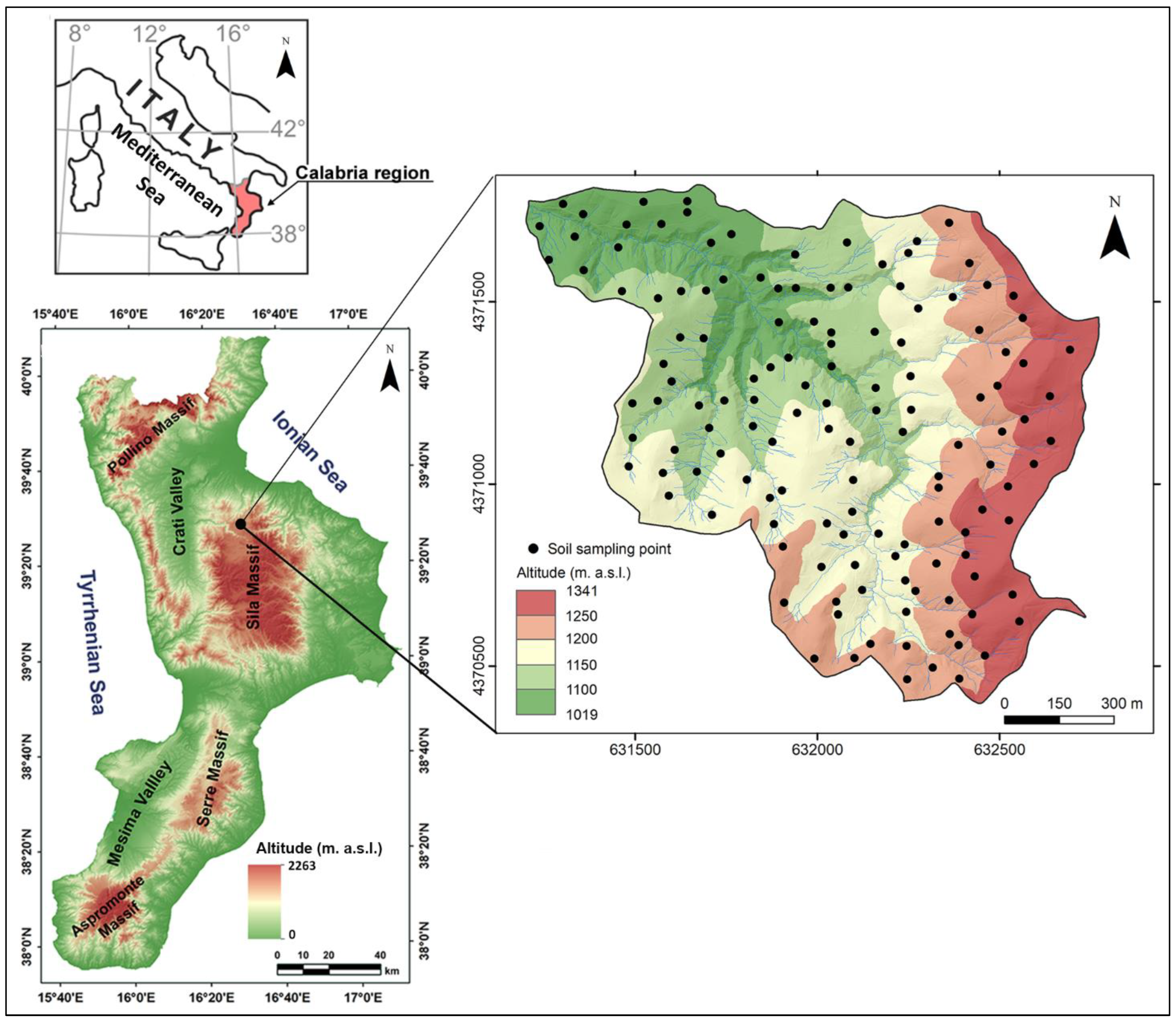
Figure 2.
Pattern of loadings multiplied by 100 of the first two principal components with values above 68.73. 68.73 is the root mean square of all the values multiplied by 100 in the matrix of PC loadings.
Figure 2.
Pattern of loadings multiplied by 100 of the first two principal components with values above 68.73. 68.73 is the root mean square of all the values multiplied by 100 in the matrix of PC loadings.
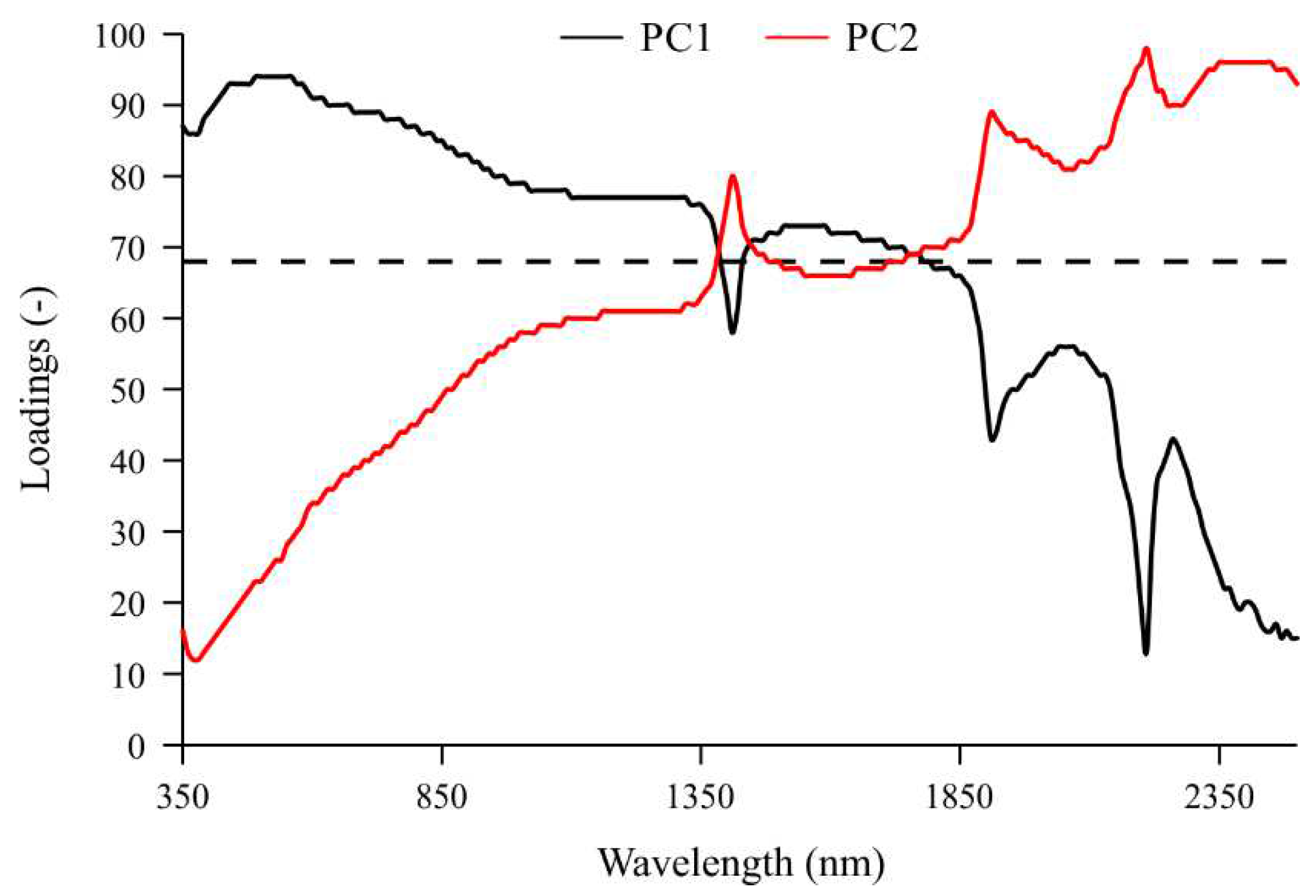
Figure 3.
Experimental variogram (filled circle) and the fitted model (solid red line) for clay content. Experimental variance (horizontal dashed line) is also showed.
Figure 3.
Experimental variogram (filled circle) and the fitted model (solid red line) for clay content. Experimental variance (horizontal dashed line) is also showed.
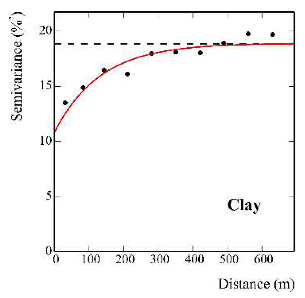
Figure 4.
Maps of clay (a) and soil organic carbon (b) content obtained with univariate ordinary kriging (white zones represent those with emergent rock).
Figure 4.
Maps of clay (a) and soil organic carbon (b) content obtained with univariate ordinary kriging (white zones represent those with emergent rock).
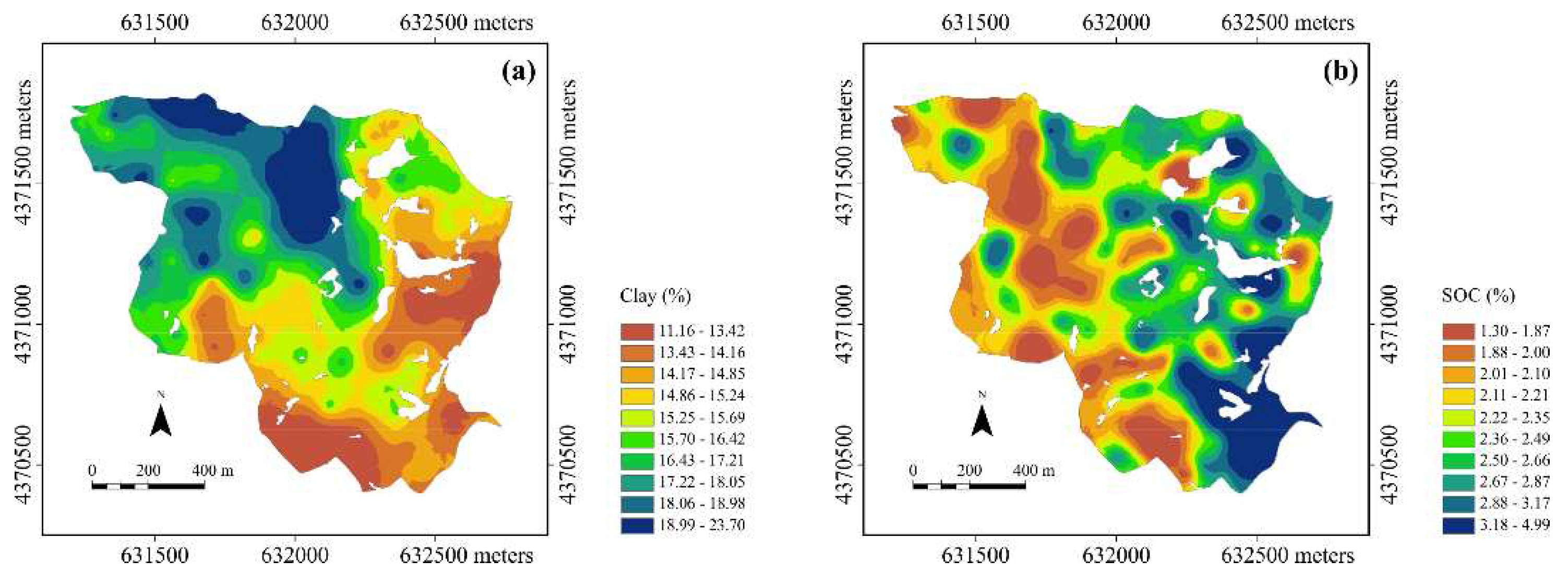
Figure 5.
Experimental variogram (filled circle) and the fitted model (solid red line) for Gaussian SOC content. Experimental variance (horizontal dashed line) is also showed. The symbol G before the variable name stands for Gaussian-transformed variable.
Figure 5.
Experimental variogram (filled circle) and the fitted model (solid red line) for Gaussian SOC content. Experimental variance (horizontal dashed line) is also showed. The symbol G before the variable name stands for Gaussian-transformed variable.
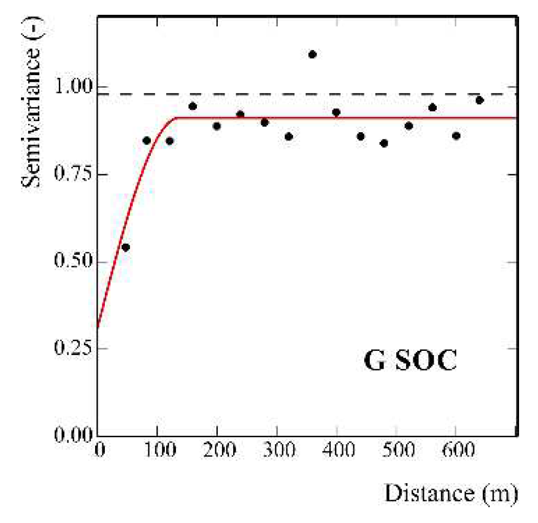
Figure 6.
Linear model of coregionalization (LMC) of PC1 and PC2. Black points are the experimental variograms; red solid lines are the fitted models, red dash-dotted lines in the cross-variogram are the hull of perfect correlation, black dashed line is the experimental variance.
Figure 6.
Linear model of coregionalization (LMC) of PC1 and PC2. Black points are the experimental variograms; red solid lines are the fitted models, red dash-dotted lines in the cross-variogram are the hull of perfect correlation, black dashed line is the experimental variance.
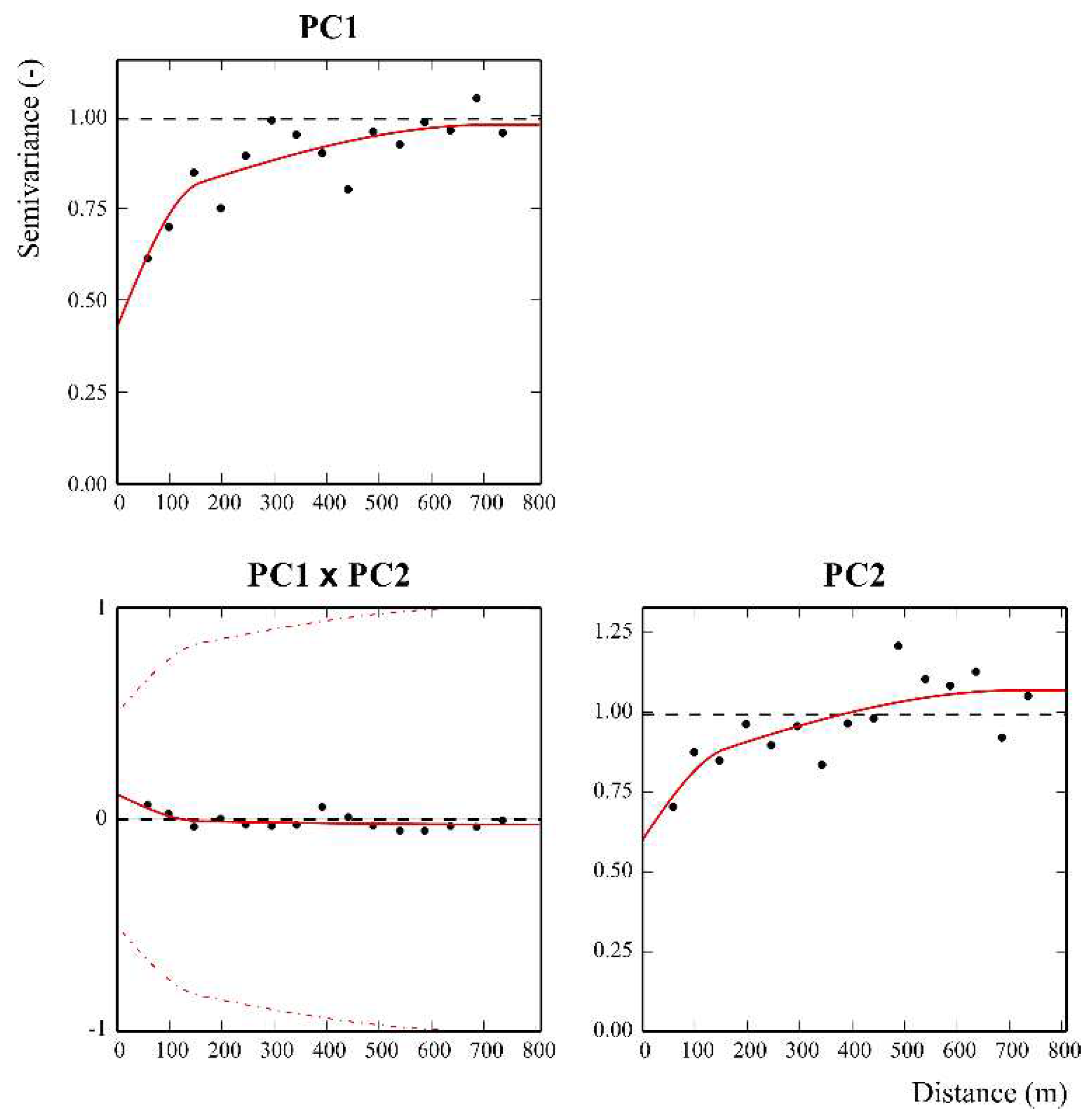
Figure 7.
Maps of the (a) first (PC1) and (b) second (PC2) principal components calculated from diffuse reflectance spectra.
Figure 7.
Maps of the (a) first (PC1) and (b) second (PC2) principal components calculated from diffuse reflectance spectra.
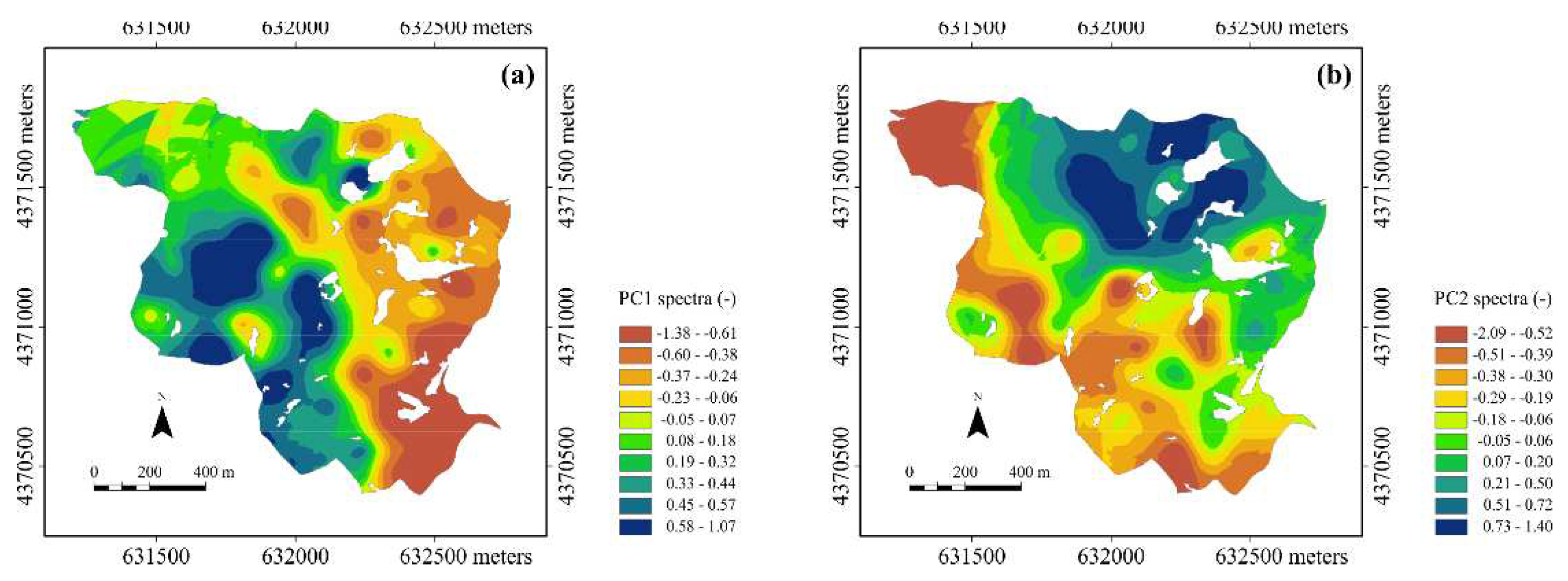
Figure 8.
Experimental variogram (filled circle) and the fitted model (solid red line) for clay concentration. Experimental variance (horizontal dashed line) is also showed.
Figure 8.
Experimental variogram (filled circle) and the fitted model (solid red line) for clay concentration. Experimental variance (horizontal dashed line) is also showed.
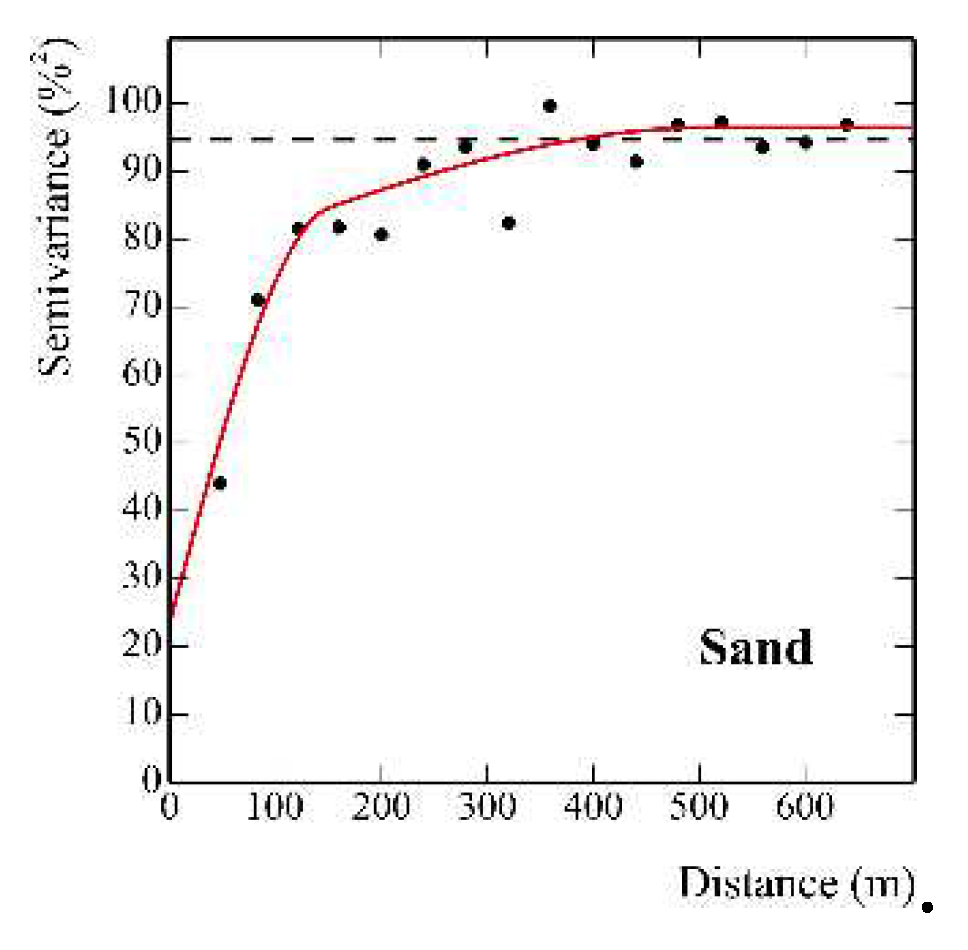
Figure 9.
Maps of the sand content estimates using the three models the three models: (a) model 1 in which the trend includes only the clay content as auxiliary variable, (b) model 2 in which the trend includes only elevation, and (c) model 3 with no trend.
Figure 9.
Maps of the sand content estimates using the three models the three models: (a) model 1 in which the trend includes only the clay content as auxiliary variable, (b) model 2 in which the trend includes only elevation, and (c) model 3 with no trend.
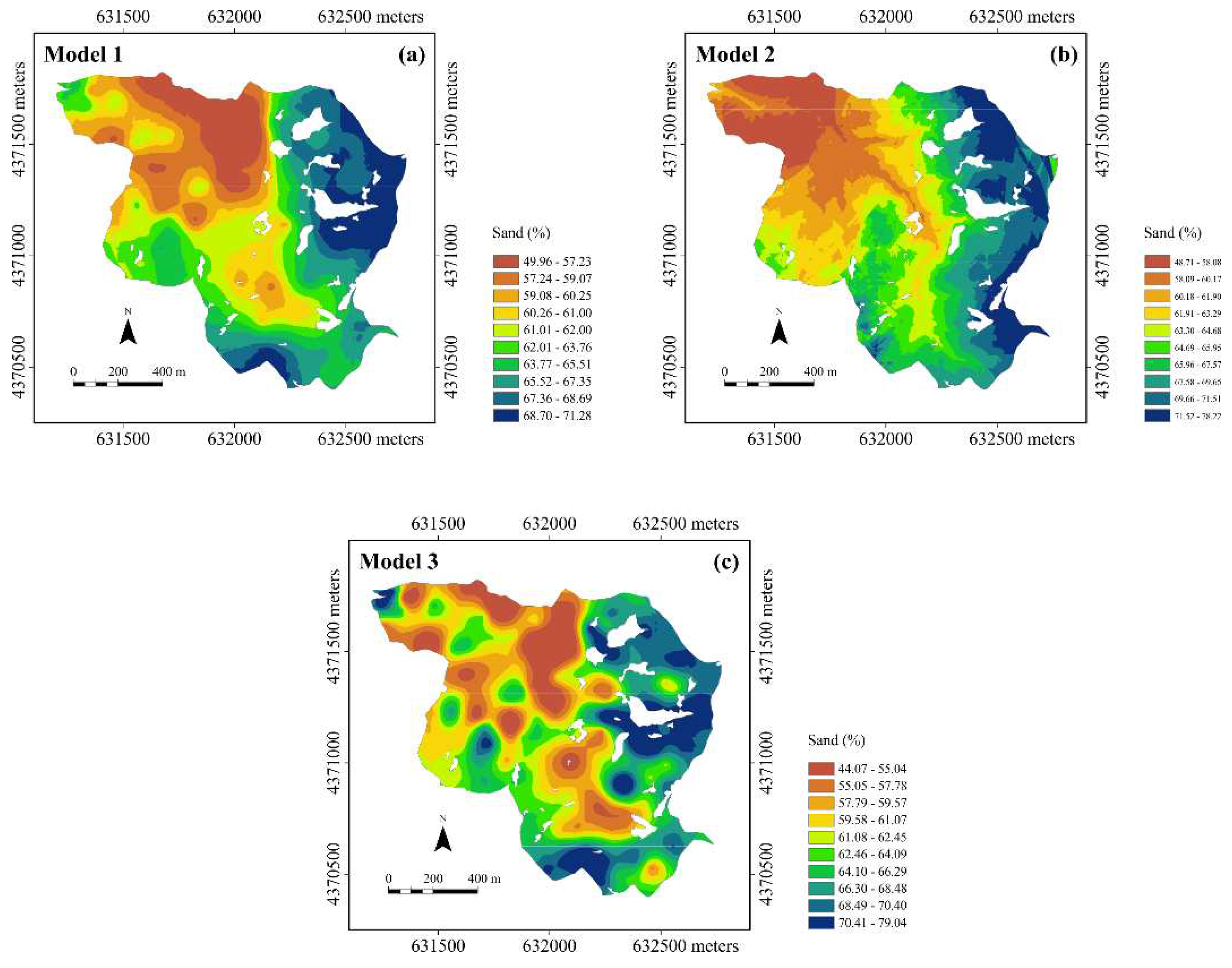
Figure 10.
Maps of the standard deviation of sand estimation using the three models the three models: (a) model 1 in which the trend includes only the clay content as auxiliary variable, (b) model 2 in which the trend includes only elevation, and (c) model 3 with no trend.
Figure 10.
Maps of the standard deviation of sand estimation using the three models the three models: (a) model 1 in which the trend includes only the clay content as auxiliary variable, (b) model 2 in which the trend includes only elevation, and (c) model 3 with no trend.
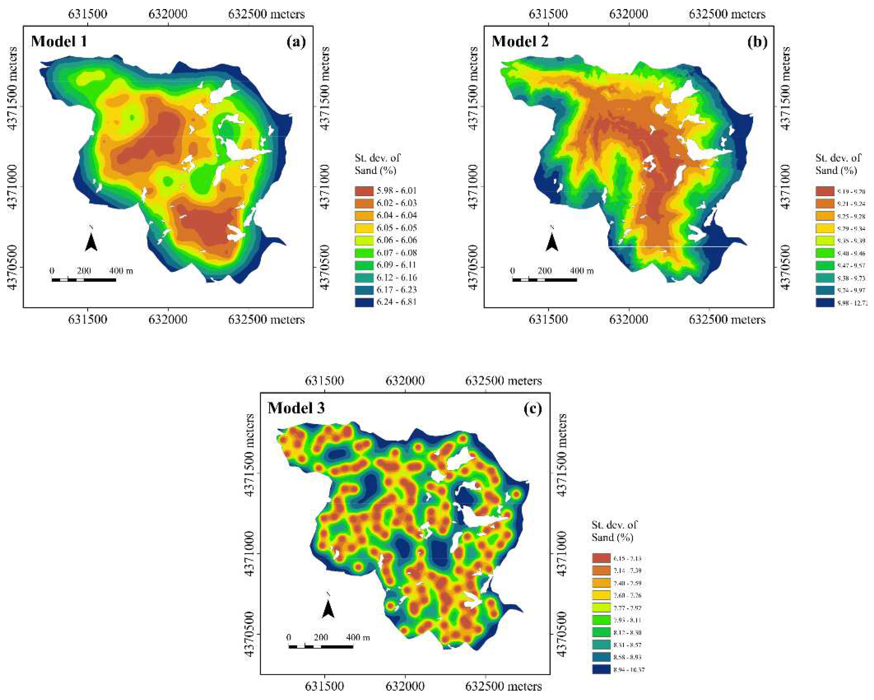

Table 1.
Summary statistics for the concentrations of sand, silt, clay, and soil organic carbon.
| Statistics | Sand (%) | Silt (%) | Clay (%) | SOC (%) |
|---|---|---|---|---|
| Minimum | 39.00 | 1.00 | 7.00 | 0.67 |
| Median | 63.00 | 22.00 | 15.00 | 2.38 |
| Mean | 62.63 | 21.34 | 16.03 | 2.66 |
| Maximum | 86.00 | 40.00 | 29.00 | 11.02 |
| Stand. Dev. | 9.73 | 6.72 | 5.04 | 1.30 |
| Skewness | -0.26 | 0.00 | 0.72 | 2.69 |
| Kurtosis | 2.86 | 3.01 | 3.11 | 15.58 |
Table 2.
Decomposition of the correlation matrix of diffuse reflectance data in principal components (PC) (only PCs with eigenvalue >1 are reported) .
Table 2.
Decomposition of the correlation matrix of diffuse reflectance data in principal components (PC) (only PCs with eigenvalue >1 are reported) .
| PC | Eigenvalue | Difference | Explained variance (%) | Cumulative explained variance (%) |
|---|---|---|---|---|
| 1 | 186.61 | 166.34 | 85.21 | 85.21 |
| 2 | 20.27 | 15.89 | 9.26 | 94.47 |
| 3 | 4.38 | 0.81 | 2.00 | 96.47 |
| 4 | 3.57 | 2.05 | 1.63 | 98.10 |
| 5 | 1.52 | 0.40 | 0.69 | 98.79 |
| 6 | 1.12 | 0.61 | 0.51 | 99.31 |
Table 3.
Summary statistics for the topographic attributes.
| Statistics | Elevation (m) |
Slope (°) |
Aspect (-) |
LS (-) |
SPI (-) |
TRI (-) |
TWI (-) |
Curvature (-) |
|---|---|---|---|---|---|---|---|---|
| Minimum | 1020.53 | 0.00 | -1.00 | 0.00 | 0.00 | 0.00 | 0.00 | -84.37 |
| Median | 1168.26 | 22.45 | 245.52 | 4.60 | 0.01 | 0.28 | 5.90 | 0.16 |
| Mean | 1171.02 | 23.40 | 213.27 | 5.05 | 0.23 | 0.31 | 5.98 | -0.02 |
| Maximum | 1340.83 | 72.86 | 360.00 | 112.63 | 1131.30 | 7.23 | 24.03 | 89.76 |
| Stand. Dev. | 65.79 | 11.44 | 104.17 | 3.36 | 5.74 | 0.19 | 1.65 | 4.47 |
| Skewness | 0.18 | 0.45 | -0.60 | 2.23 | 65.10 | 1.49 | 1.74 | -1.61 |
| Kurtosis | 2.27 | 2.90 | 2.04 | 24.17 | 6394.88 | 8.71 | 12.44 | 40.59 |
Table 4.
Correlation matrix of the coregionalization data set. In bold are the significant correlation coefficients with a probability level p<0.001.
Table 4.
Correlation matrix of the coregionalization data set. In bold are the significant correlation coefficients with a probability level p<0.001.
| Variables | Sand | Clay | SOC | PC1 | PC2 | Elevation | Slope | Aspect | LS | SPI | TRI | TWI | Curvature |
|---|---|---|---|---|---|---|---|---|---|---|---|---|---|
| Sand | 1 | ||||||||||||
| Clay | -0.76 | 1 | |||||||||||
| SOC | -0.08 | 0.02 | 1 | ||||||||||
| PC1 | -0.05 | 0.07 | -0.59 | 1 | |||||||||
| PC2 | -0.19 | 0.28 | -0.13 | -0.04 | 1 | ||||||||
| Elevation | 0.42 | -0.37 | 0.26 | -0.36 | -0.18 | 1 | |||||||
| Slope | -0.17 | 0.08 | 0.10 | -0.19 | 0.03 | -0.17 | 1 | ||||||
| Aspect | 0.18 | -0.10 | -0.01 | -0.06 | -0.04 | 0.20 | 0.05 | 1 | |||||
| LS | -0.15 | 0.05 | 0.00 | -0.18 | -0.03 | -0.14 | 0.85 | 0.04 | 1 | ||||
| SPI | -0.04 | 0.06 | -0.06 | 0.07 | -0.09 | -0.06 | -0.13 | -0.16 | 0.04 | 1 | |||
| TRI | -0.19 | 0.09 | 0.10 | -0.16 | 0.14 | -0.23 | 0.89 | 0.01 | 0.75 | -0.08 | 1 | ||
| TWI | -0.02 | 0.02 | -0.21 | 0.11 | -0.17 | 0.11 | -0.48 | -0.13 | -0.08 | 0.60 | -0.43 | 1 | |
| Curvature | -0.08 | 0.21 | 0.08 | -0.05 | 0.30 | 0.02 | -0.06 | 0.07 | -0.33 | -0.25 | -0.07 | -0.37 | 1 |
Table 5.
Automatic structure identification. T stand for trial; x, y: coordinates. For identifying the external drift, different linear combinations (T1 to T17) of the selected ten auxiliary variables were used: 1. clay; 2. SOC; 3. PC1; 4. PC2; 5. elevation; 6. slope; 7. aspect; 8. LS; 9. TRI; 9. TWI.
| (a) Identification of the order k | |||||||||||
|---|---|---|---|---|---|---|---|---|---|---|---|
| Mean Error | Mean Squared Error | Mean Rank | |||||||||
| Trial | Ring1 | Ring2 | Total | Ring1 | Ring2 | Total | Ring1 | Ring2 | Total | ||
| T1: 1 f1 | 0.260 | -0.645 | -0.197 | 44.020 | 49.220 | 46.640 | 7.043 | 6.924 | 6.983 | ||
| T7: 1 f1 f2 | 0.256 | -0.654 | -0.203 | 47.210 | 51.990 | 49.620 | 7.137 | 7.127 | 7.132 | ||
| T9: 1 f1 f2 f3 | 0.529 | -0.676 | -0.079 | 55.440 | 58.050 | 56.760 | 7.933 | 7.574 | 7.752 | ||
| T11: 1 f1 f2 f3 f4 | 0.576 | -0.601 | -0.018 | 61.680 | 63.080 | 62.380 | 8.309 | 8.052 | 8.179 | ||
| T12: 1 f1 f2 f3 f4 f5 | 0.382 | -0.632 | -0.129 | 64.530 | 69.020 | 66.790 | 8.359 | 8.054 | 8.205 | ||
| T2: 1 x y f1 | 0.600 | -1.021 | -0.217 | 48.780 | 65.710 | 57.320 | 7.301 | 8.265 | 7.787 | ||
| T8: 1 x y f1 f2 | 0.745 | -0.934 | -0.102 | 52.060 | 67.750 | 59.970 | 7.568 | 8.392 | 7.983 | ||
| T10: 1 x y f1 f2 f3 | 0.770 | -0.889 | -0.067 | 64.920 | 74.870 | 69.940 | 8.418 | 8.571 | 8.495 | ||
| T13: 1 f1 f2 f3 f4 f5 f6 | 0.734 | -1.036 | -0.158 | 77.280 | 80.660 | 78.990 | 8.967 | 8.754 | 8.860 | ||
| T14: 1 f1 f2 f3 f4 f5 f6 f7 | 0.884 | -0.888 | -0.009 | 86.140 | 96.730 | 91.480 | 9.466 | 9.244 | 9.354 | ||
| T15: 1 f1 f2 f3 f4 f5 f6 f7 f8 | 0.748 | -0.871 | -0.068 | 102.200 | 103.600 | 102.900 | 9.917 | 9.576 | 9.745 | ||
| T16: 1 f1 f2 f3 f4 f5 f6 f7 f8 f9 | 1.008 | -0.783 | 0.105 | 136.400 | 121.700 | 129.000 | 10.328 | 9.663 | 9.993 | ||
| T3: 1 f2 | 0.769 | -1.257 | -0.253 | 108.500 | 115.700 | 112.100 | 10.104 | 10.137 | 10.121 | ||
| T17: 1 f1 f2 f3 f4 f5 f6 f7 f8 f9 f10 | 1.588 | -0.874 | 0.347 | 204.800 | 163.000 | 183.700 | 11.029 | 10.188 | 10.605 | ||
| T5: 1 f3 | 1.118 | -0.735 | 0.184 | 112.900 | 119.100 | 116.000 | 10.297 | 10.476 | 10.387 | ||
| T4: 1 x y f2 | 1.408 | -1.137 | 0.125 | 116.400 | 163.900 | 140.300 | 10.510 | 10.922 | 10.717 | ||
| T6: 1 x y f3 | 1.518 | -0.531 | 0.485 | 117.900 | 158.400 | 138.300 | 10.316 | 11.080 | 10.701 | ||
| Count of measures: Ring1=1260; Ring2=1281; Total=2541 Average Neighborhood Radius: 386.57 m | |||||||||||
| (b) Covariance Identification S1 = Nugget effect; S2 = Order 1 Generalized Covariance (G.C.), Scale = 200 m | |||||||||||
| Explained/Theorical Variance Ratios | Generalized covariance | ||||||||||
| Mean square error (Q) | Ring1 | Ring2 | Rings | Jackknife test | S1 | S2 | |||||
| 0.701 | 0.959 | 1.007 | 0.984 | 0.985 | 32.380 | 5.021 | |||||
| 0.703 | 0.923 | 1.040 | 0.983 | 0.983 | 41.350 | 0.000 | |||||
| 0.717 | 1.026 | 0.831 | 0.910 | 0.894 | 0.000 | 25.150 | |||||
Table 6.
Automatic structure identification. T stand for trial. For identifying the external drift, different linear combinations (T1 to T8) of topographic attributes as auxiliary variables were used: 1. elevation; 2. TRI, 3. aspect, 4. slope, 5. LS; 6. curvature, 7. SPI, 8. TWI.
Table 6.
Automatic structure identification. T stand for trial. For identifying the external drift, different linear combinations (T1 to T8) of topographic attributes as auxiliary variables were used: 1. elevation; 2. TRI, 3. aspect, 4. slope, 5. LS; 6. curvature, 7. SPI, 8. TWI.
| (a) Identification of the order k | |||||||||||
|---|---|---|---|---|---|---|---|---|---|---|---|
| Mean Error | Mean Squared Error | Mean Rank | |||||||||
| Trial | Ring1 | Ring2 | Total | Ring1 | Ring2 | Total | Ring1 | Ring2 | Total | ||
| T1: 1 f1 | 0.525 | -0.188 | 0.165 | 89.660 | 100.500 | 95.150 | 89.660 | 100.500 | 95.150 | ||
| T2: 1 f1 f2 | 0.873 | 0.137 | 0.501 | 109.100 | 113.500 | 111.300 | 109.100 | 113.500 | 111.300 | ||
| T3: 1 f1 f2 f3 | 0.791 | 0.008 | 0.395 | 116.000 | 115.900 | 116.000 | 116.000 | 115.900 | 116.000 | ||
| T4: 1 f1 f2 f3 f4 | 0.710 | -0.011 | 0.345 | 163.300 | 142.300 | 152.700 | 163.300 | 142.300 | 152.700 | ||
| T5: 1 f1 f2 f3 f4 f5 | 0.749 | 0.080 | 0.410 | 155.400 | 141.700 | 148.500 | 155.400 | 141.700 | 148.500 | ||
| T6: 1 f1 f2 f3 f4 f5 f6 | 0.770 | 0.030 | 0.396 | 132.700 | 126.800 | 129.700 | 132.700 | 126.800 | 129.700 | ||
| T7: 1 f1 f2 f3 f4 f5 f6 f7 | 0.421 | 0.173 | 0.295 | 176.500 | 163.200 | 169.800 | 176.500 | 163.200 | 169.800 | ||
| T8: 1 f1 f2 f3 f4 f5 f6 f7 f8 | 0.179 | 0.080 | 0.129 | 204.400 | 186.800 | 195.500 | 204.400 | 186.800 | 195.500 | ||
| Count of measures: Ring1=3271; Ring2=3343; Total=6614 Average Neighborhood Radius: 493.06 m | |||||||||||
| (b) Covariance Identification S1 = Nugget effect; S2 = Order 1 Generalized Covariance (G.C.), Scale = 200 m; S3 = Spline G.C., Scale = 200 m; S4 = Order 3 G.C., Scale = 200 m | |||||||||||
| Explained/Theorical Variance Ratios | Generalized covariance | ||||||||||
| Mean square error (Q) | Ring1 | Ring2 | Rings | Jackknife test | S1 | S2 | S3 | S4 | |||
| 0.629 | 0.989 | 1.014 | 1.002 | 1.003 | 82.470 | 0.826 | 0.000 | 0.000 | |||
| 0.629 | 0.987 | 1.016 | 1.002 | 1.003 | 84.120 | 0.000 | 0.000 | 0.000 | |||
| 0.677 | 0.956 | 0.821 | 0.879 | 0.870 | 0.000 | 47.980 | 0.000 | 0.000 | |||
Table 7.
Results of cross-validation test for the three models: (1) trend includes only the clay content as auxiliary variable, (2) the trend includes only elevation, and (3) no trend. RMSSE is the root mean squared standardized error by standard deviation of kriging; r is the correlation coefficient between observation and estimation; ρ is the correlation coefficient between standardized error and estimation.
| Model | Mean error | RMSSE | r | ρ |
|---|---|---|---|---|
| 1 | -0.0215 | 0.97 | 0.78 | 0.02 |
| 2 | 0.0252 | 0.90 | 0.38 | 0.02 |
| 3 | -0.1398 | 1.13 | 0.35 | 0.16 |
Disclaimer/Publisher’s Note: The statements, opinions and data contained in all publications are solely those of the individual author(s) and contributor(s) and not of MDPI and/or the editor(s). MDPI and/or the editor(s) disclaim responsibility for any injury to people or property resulting from any ideas, methods, instructions or products referred to in the content. |
© 2023 by the authors. Licensee MDPI, Basel, Switzerland. This article is an open access article distributed under the terms and conditions of the Creative Commons Attribution (CC BY) license (http://creativecommons.org/licenses/by/4.0/).
Copyright: This open access article is published under a Creative Commons CC BY 4.0 license, which permit the free download, distribution, and reuse, provided that the author and preprint are cited in any reuse.


