Preprint
Article

Research on Improved GRU-based Stock Price Prediction Method

Altmetrics

Downloads

413

Views

33

Comments

0

A peer-reviewed article of this preprint also exists.

This version is not peer-reviewed

Submitted:

06 July 2023

Posted:

07 July 2023

You are already at the latest version

Alerts
Abstract
The prediction of stock prices holds significant implications for researchers and investors in evaluating stock value and risk. In recent years, researchers have increasingly replaced traditional machine learning methods with deep learning approaches in this domain. However, the application of deep learning in forecasting stock prices is confronted with the challenge of overfitting. To address the issue of overfitting and enhance predictive accuracy, this study proposes a stock prediction model based on GRU (Gated Recurrent Unit) with reconstructed datasets. This model integrates data from other stocks within the same industry, thereby enriching the extracted features and mitigating the risk of overfitting. Additionally, an auxiliary module is employed to augment the volume of data through dataset reconstruction, thereby enhancing the model’s training comprehensiveness and generalization capabilities. Experimental results demonstrate a substantial improvement in prediction accuracy across various industries.
Keywords: 
Subject: Computer Science and Mathematics  -   Artificial Intelligence and Machine Learning

1. Introduction

With the development and gradual refinement of the corresponding systems in Chinese stock markets, an increasing number of individuals have grown interested in participating in stock market investment. However, due to stock prices are influenced by various factors such as policy adjustments and company performance[1], which are themselves highly unstable, accurately predicting the future trend of stock prices becomes crucial in helping investors achieve higher returns and better manage potential risks. Furthermore, predicting stock prices can also help enterprises make better investment decisions, ultimately increasing their value and profitability. Therefore, predicting the future trend of stocks has become one of the most attractive research topics in the academic community.
There are various methods for predicting stocks, which can be broadly classified into fundamental analysis and technical analysis. Currently, technical analysis methods commonly used at home and abroad can be roughly divided into two categories: econometric methods and machine learning (ML) methods. The mainstream econometric models, such as Autoregressive Moving Average (ARMA) [2] model, Autoregressive Integrated Moving Average (ARIMA) [3] model, Generalized Autoregressive Conditional Heteroscedasticity (GARCH) model, Vector Auto Regression (VAR) model and so on, have been proven effective in predicting the stock market according to literature. Although econometric methods are more objective in nature and supported by appropriate theories, their effectiveness with regard to stock market prediction relies on the strictness of their underlying assumptions, and they are only applicable to linearly structured data. However, given that the stock market is a dynamic system influenced by various factors and is often characterized by a series of complex and nonlinear features, traditional econometric prediction methods are restricted by certain limitations and are not well-suited to the analysis of complex, high-dimensional, and noisy financial time series.
To achieve better results, some complex and nonlinear ML methods such as Support Vector Machines (SVM) [4], Genetic Algorithms (GA) [5], Fuzzy Logic (FL) [6] and hybrid models [7] have been widely used by researchers in stock price prediction. Compared to traditional econometric methods, ML requires fewer assumptions and has a significant advantage in extracting data features, thus being able to handle nonlinear and nonstationary data. Wu et al. [8] applied a Backpropagation Neural Network (BPNN) to predict the ups and downs of the Shanghai Composite Index, and the results indicated that the model was effective in predicting the Chinese stock market. Ticknor [9] used BPNN to predict the trend of Microsoft and Goldman Sachs stock prices, and the effectiveness of the model was confirmed. Zhang and Lou [10] used BPNN to predict stock prices, and after empirical testing, achieving an accuracy rate of 73.29% in predicting stock prices. Tay and Cao [11] studied the application of Support Vector Regression (SVR) in stock market prediction, demonstrating the superiority of SVR in stock market prediction. Kim [12] used support vector machines (SVM) to classify the daily directional changes in the Korean stock market index (KOSPI) and compared the results with those of Neural Networks (NN) and Case-Based Reasoning (CBR) predictions, showing that SVM has better predictive performance. Ran Yangfan and Jiang Hongxun [13] used BPNN and SVR to construct a stock price prediction model, and the results showed that the SVR stock price prediction model had smaller errors and higher accuracy in predicting stock price trends. However, Shallow ML algorithms possess relatively simple structures and may exhibit insufficient handling capabilities for raw data. Moreover, such algorithms are frequently susceptible to issues such as local optima or overfitting and may experience slow convergence during real-world application scenarios.
To address the above issues associated with ML, researchers have resorted to the application of deep learning methods for stock price prediction. Deep learning, proposed by Hinton and Salakhutdinov [14], has been widely adopted in modeling time-series data. Singh and Srivastava [15] used Deep Neural Network (DNN) to predict the NASDAQ index, achieving 17.1% higher accuracy as opposed to Radial Basis Function Neural Network (RBFNN), demonstrating that deep learning can enhance the accuracy of stock price prediction. Additionally, Persio and Honchar [16] utilized Multilayer Perceptron (MLP) and Convolutional Neural Networks (CNN) in predicting the opening and closing prices of the S&P500 index on the next day and concluded that CNN exhibits smaller prediction errors compared to MLP. Kraus et al. [17] integrated DNN, Gradient-Boosted Trees, and Random Forests to predict the future returns of the S&P500 index stocks over a selected time period. To predict high-frequency stock market trends, Chong et al. [18] combined DNN with three unsupervised feature extraction methods, including Principal Component Analysis (PCA), Autoencoder, and Restricted Boltzmann Machine. Cui [19] used Deep Belief Networks (DBN)to prognosticate future stock price changes, recording better performance in comparison to BPNN and RBFNN. Similarly, Liu [20] combined fuzzy theory with DBN to propose a fuzzy deep-learning network model for stock price prediction, which exhibited satisfactory prediction performance and broad research prospects through experimental results. Li et al. [21] introduced intrinsic plasticity into DBN, enabling the model to have adaptive capabilities, and the results showed that the prediction accuracy of stock closing prices was significantly improved. Tsantekidis et al. [22] encoded sequence data with an encoder and then used CNN for prediction, illustrating that CNN is better suited for predicting stock trends compared to other methods such as MLP and SVM. Hsieh et al. [23] first utilized wavelet transform to decompose stock prices for noise elimination, and then used Recurrent Neural Networks (RNN) optimized by artificial bee colony algorithm to predict stock prices in real-time. Rather et al. [24] proposed a hybrid predictive model comprising Autoregressive Moving Average models, Exponential Smoothing models, and RNN to predict stock returns, with better prediction performance than a single RNN. Qin et al. [25] proposed a double-stage attention-based RNN model that adaptively extracts relevant input features for prediction, and displayed the model is more effective in stock dataset prediction than other techniques. Sim, Kim, and Ahn [26] established a CNN-based stock price prediction model for the S&P500 index and compared the accuracy of the model with Artificial Neural Networks (ANN) and SVR, and the experimental results showed that CNN is an ideal choice for developing stock price prediction models. Furthermore, Chen et al. [27] proposed a CNN-based stock trend prediction model dependent on graph convolutional features and verified the superiority of the model using six randomly selected Chinese stocks.
To mitigate the prevalent challenges of gradient vanishing or exploding, and long-term dependencies in neural networks, Long Short-Term Memory (LSTM) neural network was proposed by Hochreiter and Schmidhuber [28] has been widely used for time-series prediction. Compared with traditional RNN, LSTM is better able to solve the problem of long-term dependencies by retaining information previously processed during training. Persio and Honchar [16] compared the performance of RNN, LSTM, and GRU (Gated Recurrent Unit) in the prediction of Google stock prices and found that LSTM neural networks have advantages in stock price prediction. Yang and Wang [29] extended their research to 30 global stock indices and constructed LSTM to compare short-term, medium-term, and long-term prediction performance. According to the results, LSTM demonstrated higher prediction accuracy compared to the econometric method ARIMA and ML methods SVR and MLP across all indices for different periods. Deep learning has been proven to produce highly accurate predictions across a broad range of applications. However, the serious issue of overfitting[30] is a significant concern in deep learning, particularly when the training dataset is small relative to the complexity of the model. In such situations, the deep learning model may memorize the training data rather than generalize to new inputs, leading to poor performance on unseen test data. Despite the availability of various regularization techniques to mitigate overfitting, the problem remains a significant challenge in deep learning, and ongoing research is focused on developing more effective solutions to this critical issue.
The purpose of this paper is precisely to address this problem as well. The main research content of this paper is outlined as follows:
1. A stock prediction framework is proposed, employing data augmentation methods to increase the dataset to expand the dataset and mitigate the risk of overfitting.
2. The performance of the model is validated employing real stock data from several industries in China, resulting in superior outcomes and reduced errors compared to existing methodologies, thus enhancing the accuracy of stock prediction.
In this study, we introduce an enhanced model based on GRU to forecast stock price trends by incorporating key factors that influence stock prices, such as industry trends. Our objective is to enhance the performance of the model and minimize prediction errors. Furthermore, we construct a refined dataset by integrating data from other stocks within the same industry with the dataset of the target stock to improve the accuracy of stock price prediction. A comparative analysis of our proposed approach against the performance of the GRU model demonstrates its superior predictive capabilities and reduced margin of error. The novelty of our research lies in the unique application of industry-wide stock data, which captures comprehensive industry trends and distinctive features. The augmented dataset not only mitigates the risk of model overfitting but also significantly enhances the precision of stock price forecasting for the target stock.

2. Materials and Methods

Time series index data itself is an important and direct source of bias for predicting stock market indices. A simple model involves utilizing historical target data as input to forecast future movements, as depicted in the figure below. The left side represents the input of historical stock data, and the output is future stock prices. However, deep learning models require a large amount of data to make effective predictions. In the example presented in this paper, the number of data points is less than 10,000, which can lead to the problem of overfitting, where the model is excessively trained to give high training accuracy but low testing accuracy. To mitigate the problem of overfitting, it becomes imperative to augment the relevant dataset without altering the original data. This augmentation is based on the concept of incorporating an auxiliary module, as proposed in Section 2.2. This auxiliary module employs a restructured relevant dataset to assist the prediction module in making accurate predictions.
Figure 1. A simple deep-learning model
Preprints 78736 g001

2.1. GRU

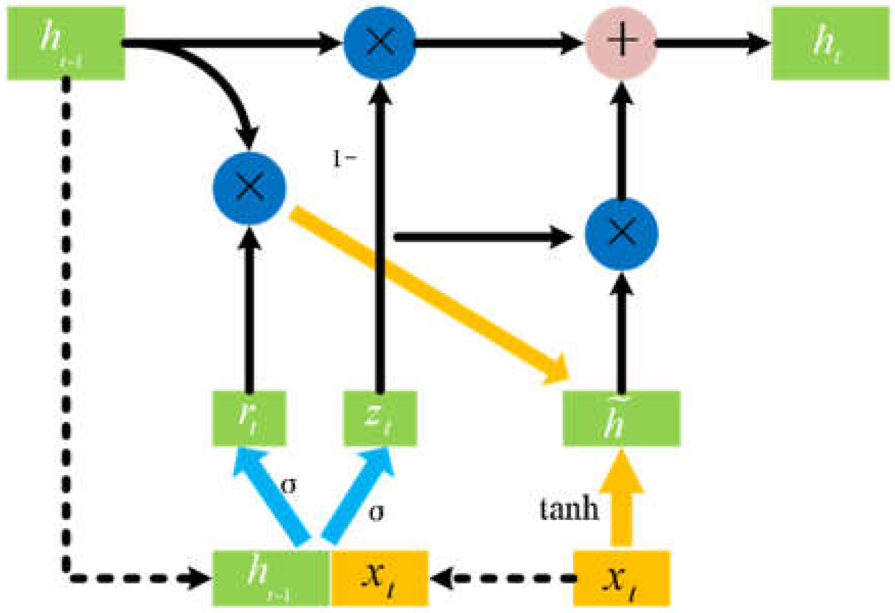
Since this paper focuses on particularly time series prediction, the commonly used deep learning method is RNN. However, RNN can encounter issues such as gradient explosion and vanishing, particularly when learning long-term dependencies in the data. To resolve these problems, subsequent studies have proposed the LSTM, which improves the gradient flow within the network by employing a gating mechanism. GRU is a simplified version of LSTM, reducing the three gates in LSTM to two. Consequently, GRU exhibits enhanced proficiency in capturing and learning long-term dependencies in time series data, while also reducing model complexity and computational costs, thus providing superior training efficiency. The improved ability of GRU to handle long-term dependencies in time series data makes it the preferred choice. Additionally, GRU demonstrates lower storage requirements, rendering it suitable for processing large-scale datasets. Therefore, the basic GRU model was selected as the primary model in this study. The architecture of the GRU model is illustrated in Figure 2.
Figure 2. GRU architecture block diagram
Preprints 78736 g002
r t = σ ( W r x t + U r h t 1 + b r )
z t = σ ( W z x t + U z h t 1 + b z )
h t ˜ = tanh ( W h x t + U h ( r t h t 1 ) + b h )
h t = z t h t 1 + ( 1 z t ) h t ˜
Here, represents the element-wise product formula; W r and W z are the weight matrices of the r t gate and the z t gate, respectively; U h represents the weight matrix for output; x t represents the input data at time t; h t ~ and h t represent the candidate state and output state at time t; b r , b z and b h are constants. σ and tanh are the sigmoid and tanh activation functions, respectively, used to activate the control gates and candidate states.
After the information enters the GRU unit, the process of flow transmission includes the following steps:
(1) Concatenate the input data x t at time t and the output of the hidden layer h t 1 at time t-1. The output signal of the reset gate r t is obtained by formula (1).
(2) The output signal of the update gate z t is obtained by formula (2).
(3) The current state hidden unit candidate set h t ~ is obtained by formula (3), which mainly integrates the input data x t and the hidden layer state at time t-1 after filtering by the reset gate.
(4) The output of the hidden layer h t at time t is obtained by formula (4), which represents forgetting the hidden layer information h t 1 passed at time t-1 and selecting important information from the candidate hidden layer at time t.

2.2. The Proposed model architecture

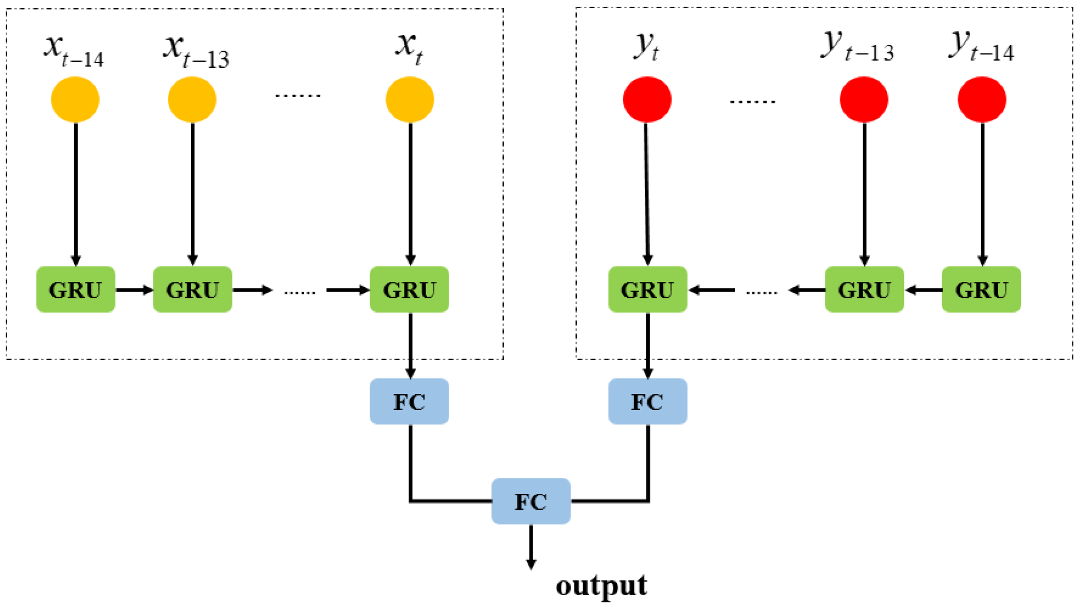
To address the problem discussed in the preceding context, this paper proposes a combined model, as illustrated in Figure 3, based on the GRU algorithm. The left module takes the historical data of the target stock to be predicted as input and uses the GRU module to process it. On the other hand, the right module serves as the auxiliary module, which takes input data constructed using the approach described in section 2.5 of this paper. Its function is to fine-tune the left prediction module by incorporating features related to the relevant industry of the target stock, thereby avoiding overfitting and improving the effectiveness of the prediction.
In this model, both the target stock prediction module and the auxiliary module are trained using the GRU model. Each module produces an output through a fully connected layer. These two outputs are subsequently inputted into another fully connected layer to obtain the final output, representing the predicted price of the target stock.
Figure 3. Proposed stock price prediction architecture
Preprints 78736 g003

2.3. Datasets

Based on the formula for sample size selection, when N 3 , one-by-one sampling is used; when 3 < N 300 , random sampling is conducted with a sample size of N + 1 ; when the total sample size N > 300 , random sampling is conducted with a sample size of N 2 + 1 .
In this experiment, stock data was chosen based on the industry categorization. An L2 industry typically contains only around 100 samples. Hence, this study employed a sampling quantity equation to determine the selection of sample stock data. The sample size derived from the formula for the selected industry was less than ten or just over ten. To ensure experimental consistency, ten stocks from the same industry as the target stock to be predicted were selected in each experiment. Using these ten stocks can achieve results similar to those generated by the entire industry. In this experiment, the following five parameters of the stock were considered: opening price (open), highest price (high), lowest price (low), closing price (close), and trading volume (vol). These ten stocks were chosen to represent the trend of the entire industry, as their features have a relatively significant impact on the information of the target stock to be predicted in this study.
The dataset chosen for the research encompasses industries that are closely related to our daily lives, including liquor, pharmaceutical retail, banking, and film and television. A total of 1146 historical data points containing the aforementioned five parameters for each of the stocks of these companies from April 10, 2018, to December 23, 2022 were chosen. Details of the target stock to be predicted and the selected related stocks are shown in the Table 1.
Table 1. Target Stocks and Related Stocks Table
Industry Target Stocks Related Stocks
Baijiu Gujing Gongjiu Maotai Guizhou, Wuliangye, Yanghe Dis-tillery, Luzhou Laojiao, Fenjiu, Shunxin Agriculture, Jinshiyuan, Kouzi Jiu, Shui-jingfang, Yingjia Gongjiu, Jiuguijiu.
Pharmaceutical Business Laobaixing Shanghai Pharmaceutical, Huadong Medicine, Jiuzhou Tong, Da Can Lin, China National Pharmaceutical Group Corp., China National Prescription Drug Co., Ltd., China Medical System Holdings Limited, Haiwang Biology Co., Ltd., Yi Xin Tang, Taiyangneng
Bank Bank of Communications Industrial and Commercial Bank of China (ICBC), China Construction Bank (CCB), Agricultural Bank of China (ABC), Bank of China (BOC), China Merchants Bank (CMB), Industrial Bank Co Ltd (IB), Shanghai Pudong Development Bank (SPDB), Ping An Bank, China CITIC Bank, China Minsheng Banking Corp Ltd
Cinema Chain Dongyanghengdian Film and Television City Enlight Media, China Film Group Corpo-ration, Huace Film & TV, Alpha Group Co., Ltd., Huayi Brothers Media Corp, Bei-jing Culture Co., Ltd., Central Motion Pic-ture Corporation, Huayi Brothers Fashion Group Co., Ltd., Shanghai Film Group Corporation, Bona Film Group Limited.

2.4. Normalization

The notable differences observed among the five parameters of each type of stock may impact the optimization of the trained model weights in the later stages. To eliminate such impacts, the present study employed a normalization formula (5) to standardize the data within the range of [0,1].
X i n = X i X min X max X min

2.5. Construction of the auxiliary module dataset
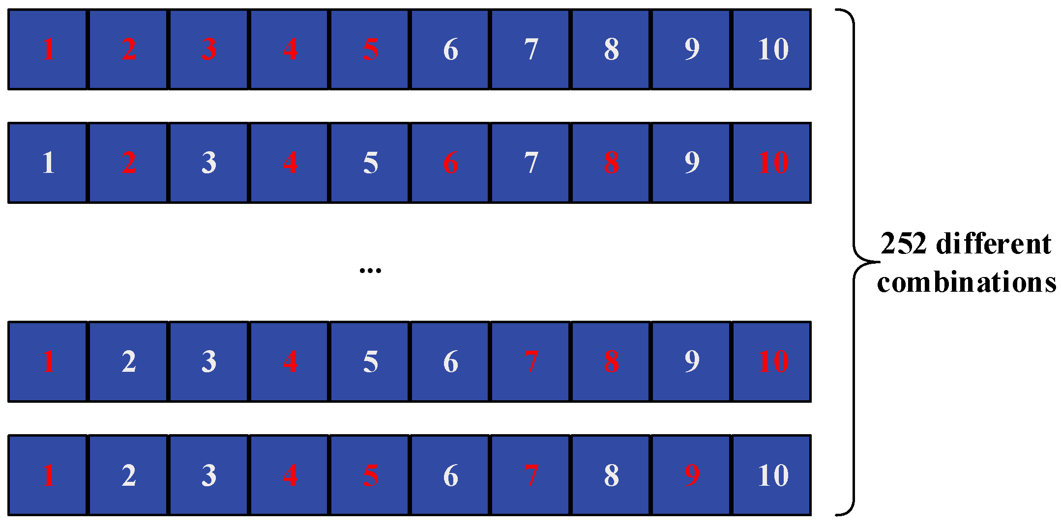
The core focus of this model lies in the construction of the auxiliary module dataset. Ten stocks were chosen by using the aforementioned methods and subsequently normalized. For this experiment, two distinct approaches were employed to handle the historical data of these ten stocks. The data was reconstructed[31] using these two approaches, and the experiment was conducted on the resulting datasets.
1. Fixed selection: Five stocks were randomly selected from the ten chosen stocks, and the average of their respective parameters was taken to create the dataset required for the experiment.
2. Random selection: For each trading day, five stocks were randomly selected from the ten chosen stocks, and the average of their respective parameters was taken to create the dataset required for the experiment. This process is illustrated in Figure 4.
Figure 4. Data selection method diagram
Preprints 78736 g004
As this study focuses on predicting of the target stock, the historical data of the target stock is the main input. In this experiment, a rolling time window of 15 is set, which means that the historical data of the first 15 lagged days is used as input, and the data of the 16th day is used as output. Then the data of the 2nd to 16th day is used as input, and the data of the 17th day is used as output, following this pattern. This process is illustrated in the figure. To validate the effectiveness of the model, the window size can also be set to 5, 10, or 20 days during the experiment. In this specific experiment, a window size of 15 days is used to assess the model’s performance.

2.6. Evaluation Parameter

To evaluate the model prediction results, this article selected three evaluation metrics, including Root Mean Square Error (RMSE), Mean Absolute Error (MAE), and Mean Absolute Percentage Error (MAPE). The calculation methods of each evaluation metric are as follows:
(1) RMSE
RMSE is commonly utilized to assess the extent of deviation between predicted outcomes and actual data. A smaller RMSE value indicates a higher accuracy of the prediction model. The RMSE is mathematically defined as follows:
R M S E = 1 N i = 1 N ( y i y i ) 2
(2) MAE
MAE refers to the average absolute deviation between the arithmetic mean and individual observed values. A smaller MAE value indicates higher prediction accuracy. The MAE is mathematically defined as follows:
M A E = 1 N i = 1 N y i y i
(3) MAPE
MAPE is utilized to quantify the average deviation between the predicted value and the actual value. A lower MAPE value implies a higher level of prediction accuracy. The MAPE is mathematically defined as follows:
M A P E = i = 1 N y i y i y i × 100 N

3. Results

This section presents experimental findings obtained by employing the model proposed in section 2.2 to analyze stock data across multiple industries. Various industries that are pertinent to individuals’ daily lives were selected, including liquor, pharmaceutical retail, banking, and film and television companies. The input utilized two modules: the historical data of the target stock and a dataset constructed using historical data from related stocks. The output consisted of the predicted price of the target stock for the following day.
The experimental results are divided into two parts, as per the two data processing methods proposed in the preceding section: fixed selection and random selection. A comparison of results was made with the classical GRU model, and three evaluation metrics, namely RMSE, MAE, and MAPE, were used to validate the model’s output against the actual prices.
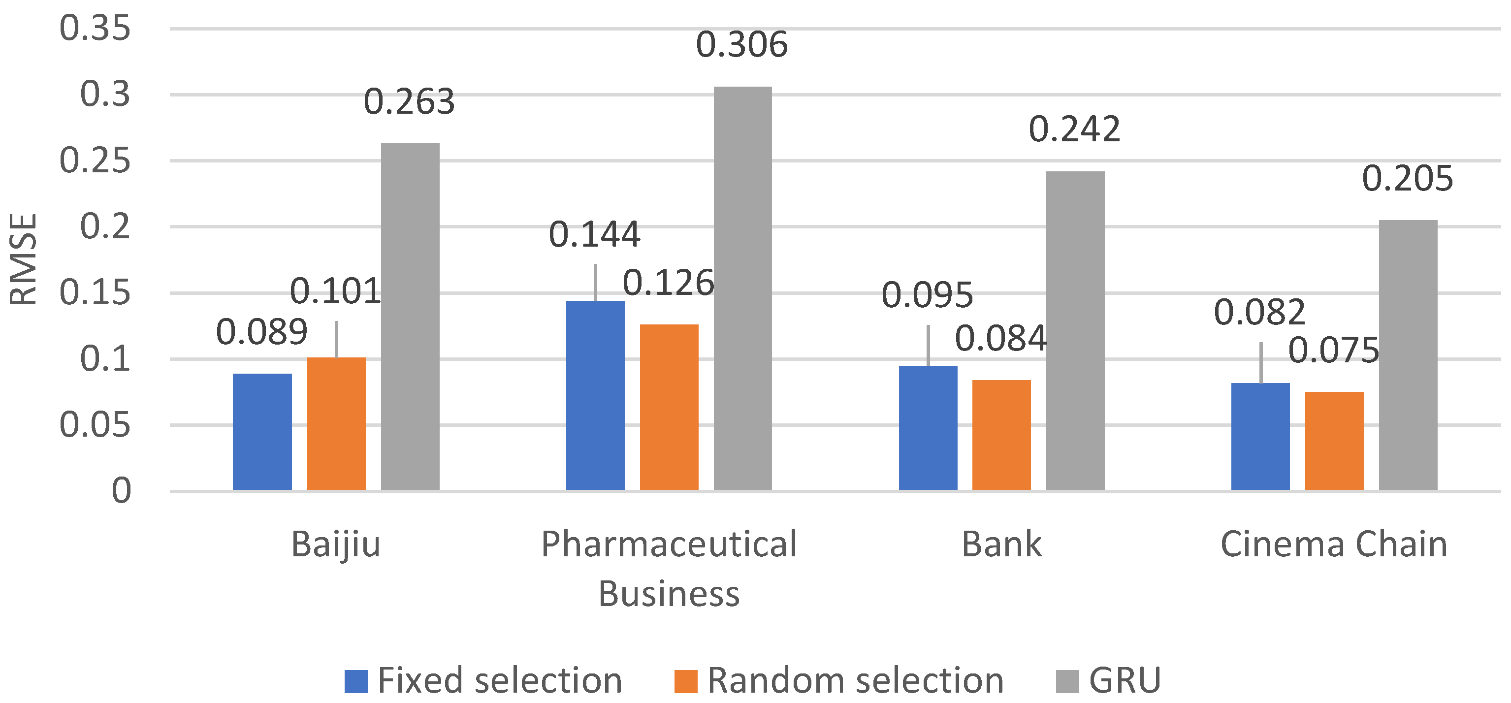
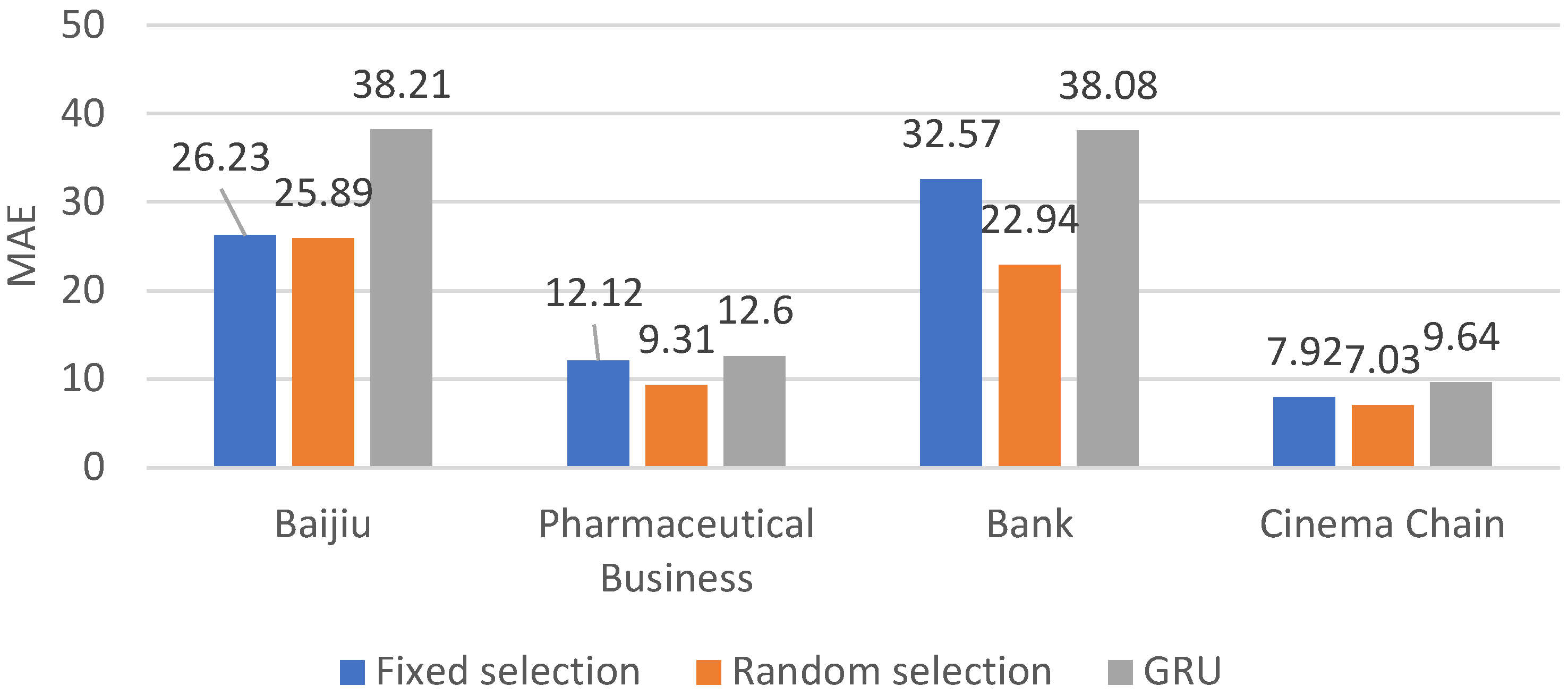
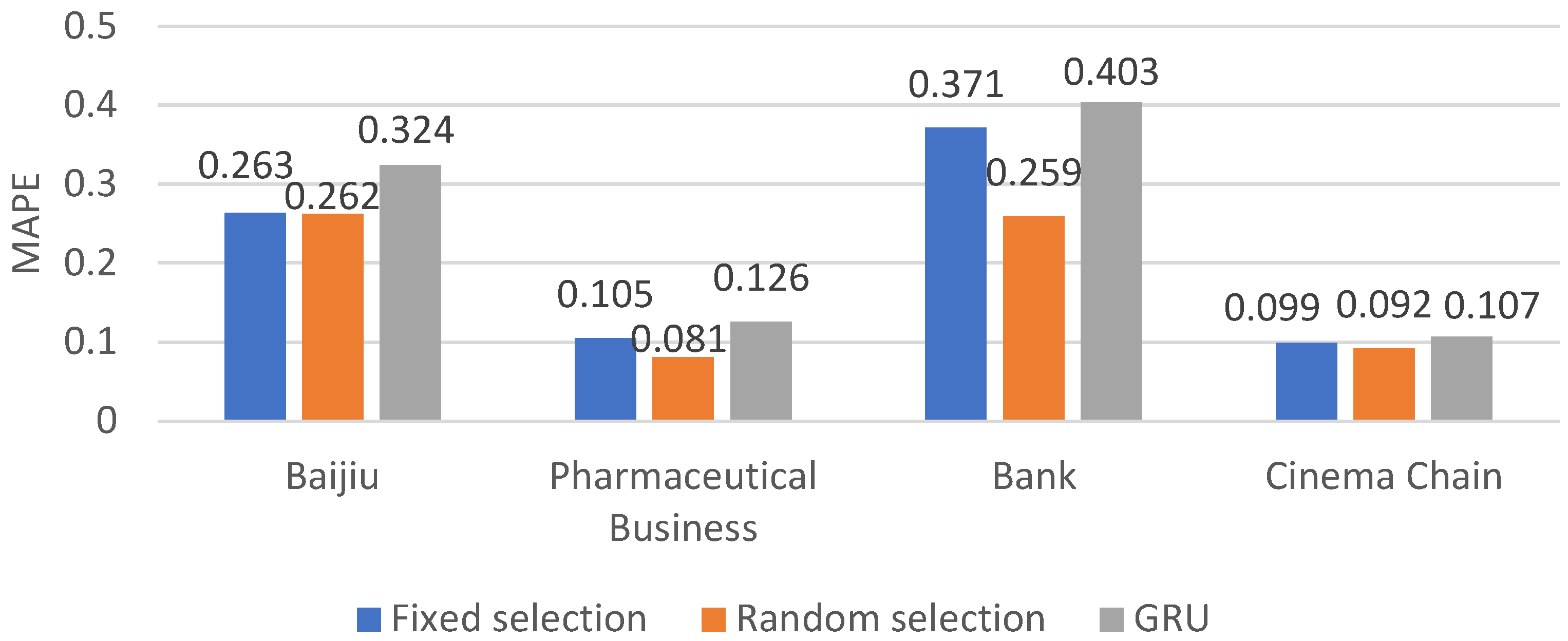
The data set was split into two subsets, with 80% as the training set and 20% as the testing set. The results are depicted in Table 2, Table 3 and Table 4 and in Figure 5, Figure 6 and Figure 7. As depicted in the figure or table, the aforementioned paper introduces two methods that exhibit superior performance compared to the classical GRU across all three metrics: RMSE, MAE, and MAPE. Notably, in terms of RMSE, the errors across all four industries are reduced by more than twofold. Moreover, the Random selection method delivers the best results in both MAE and MAPE for the banking industry, achieving a reduction in errors by 15.14 percent and 0.144, respectively.
Table 2. The RMSE of the four industries under three different experimental methods
Baijiu Pharmaceutical Business Bank Cinema Chain
Fixed selection 0.089 0.144 0.095 0.082
Random selection 0.101 0.126 0.084 0.075
GRU 0.263 0.306 0.242 0.205
Table 3. The MAE of the four industries under three different experimental methods
Baijiu Pharmaceutical Business Bank Cinema Chain
Fixed selection 26.23 12.12 32.57 7.92
Random selection 25.89 9.31 22.94 7.03
GRU 38.21 12.60 38.08 9.64
Table 4. The MAPE of the four industries under three different experimental methods
Baijiu Pharmaceutical Business Bank Cinema Chain
Fixed selection 0.263 0.105 0.371 0.099
Random selection 0.262 0.081 0.259 0.092
GRU 0.324 0.126 0.403 0.107
Figure 5. The RMSE of the four industries under three different experimental methods
Preprints 78736 g005
Figure 6. The MAE of the four industries under three different experimental methods
Preprints 78736 g006
Figure 7. The MAPE of the four industries under three different experimental methods
Preprints 78736 g007

3.1. The experimental results of the Fixed selection method
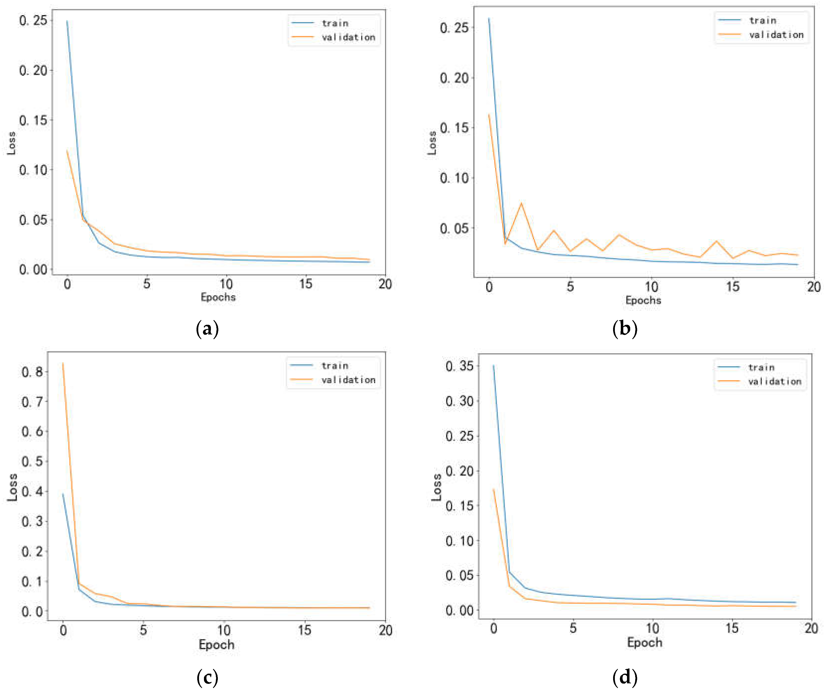
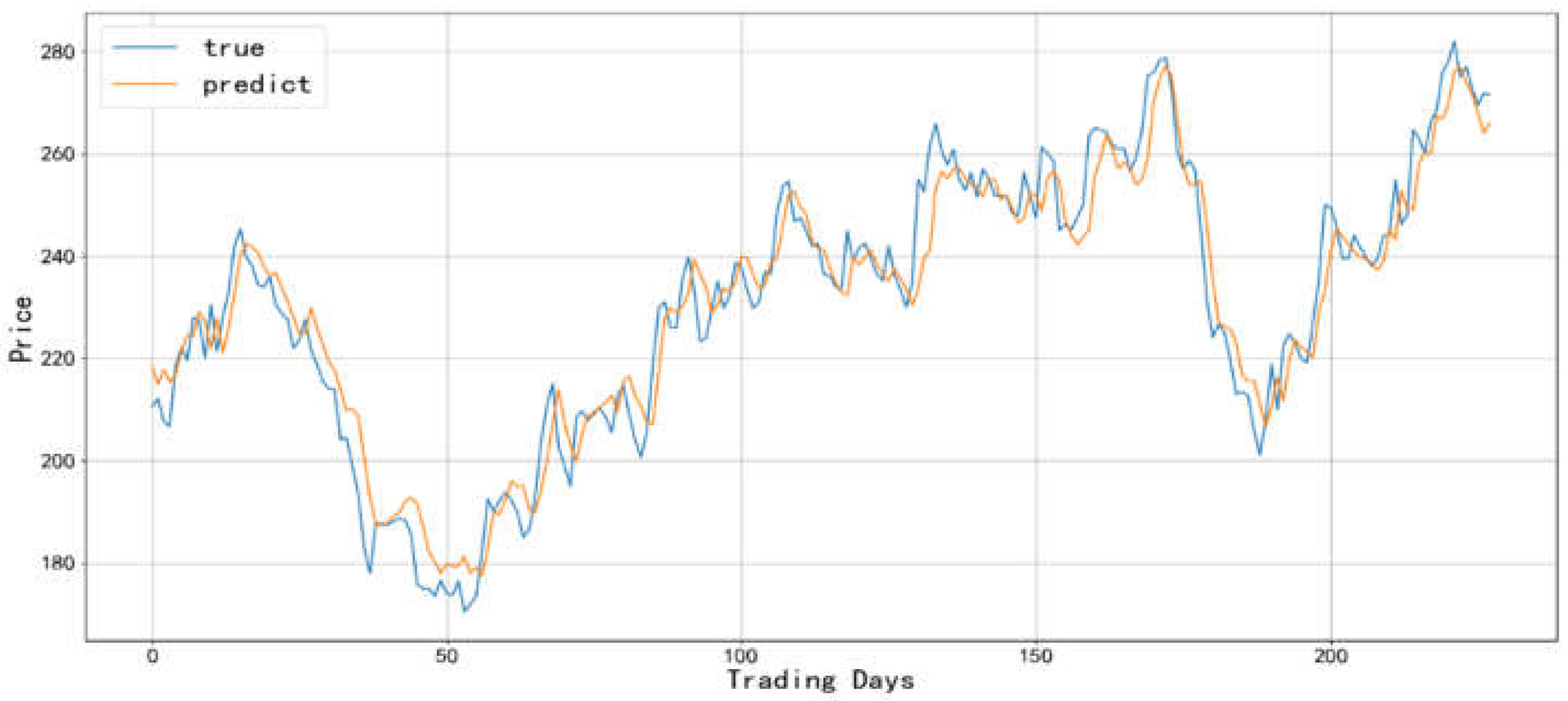
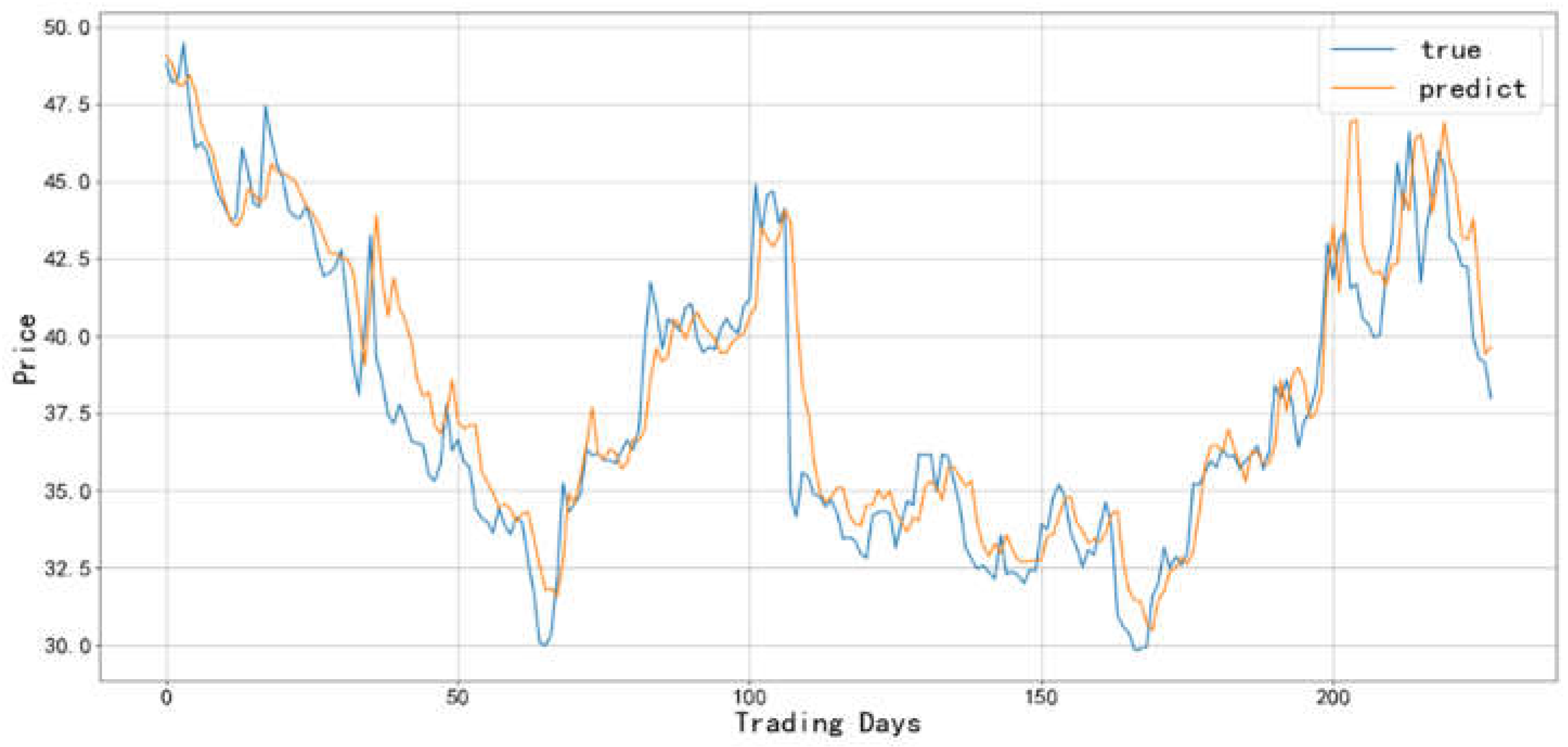
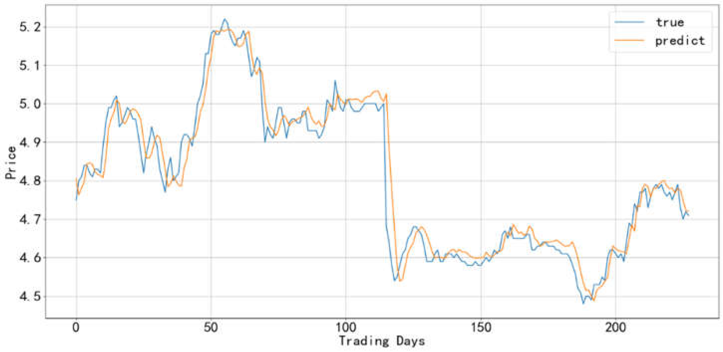
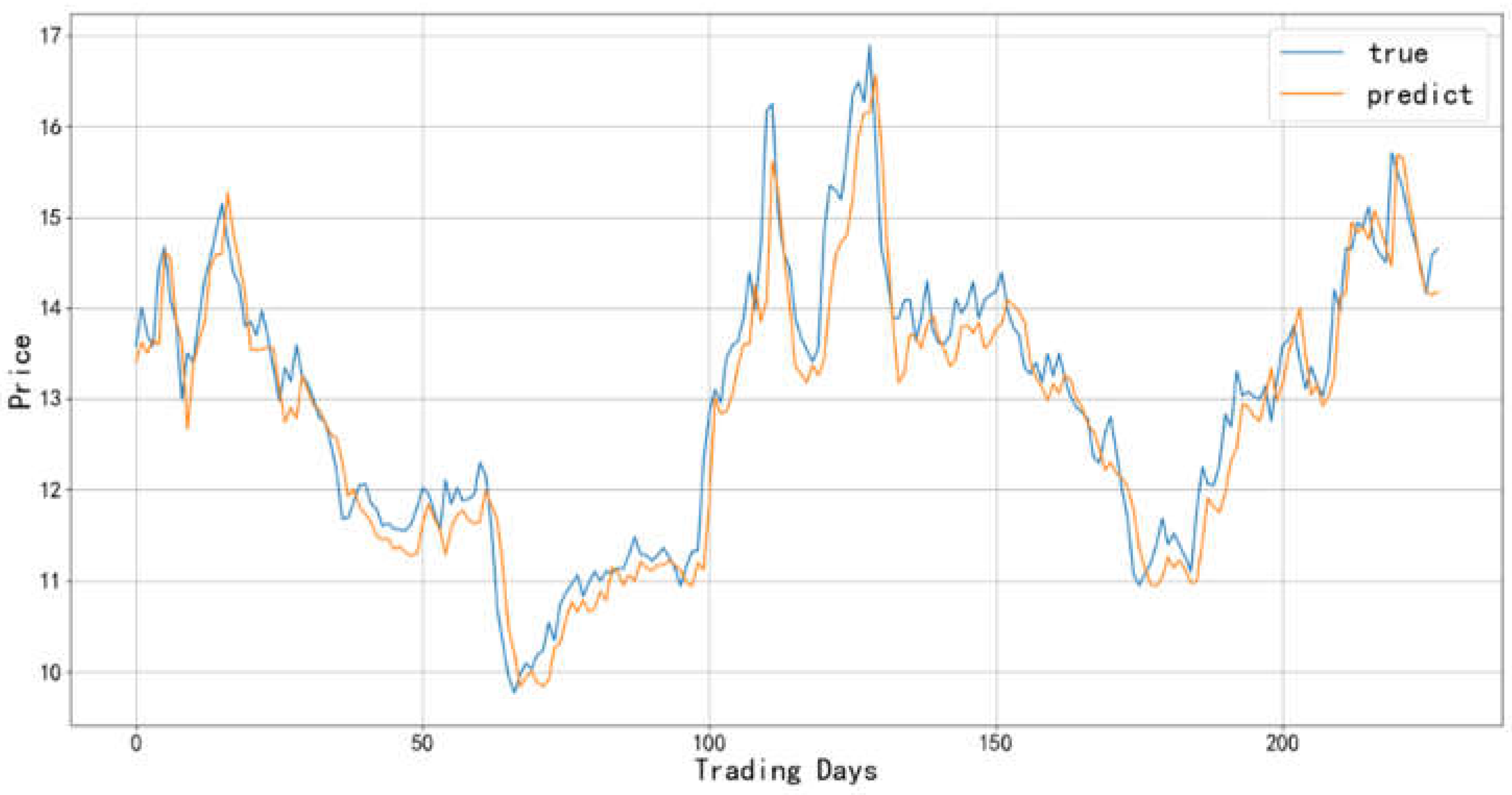
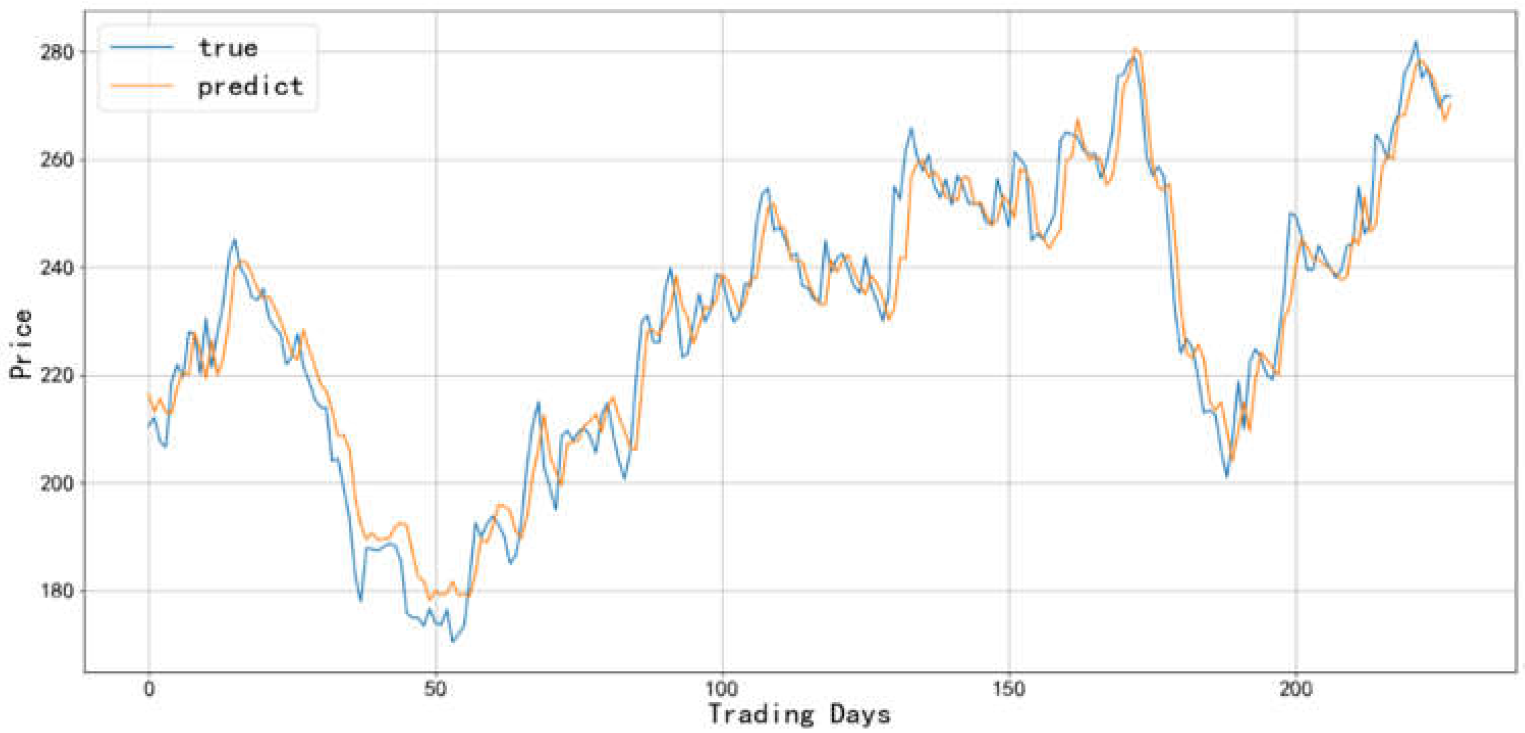
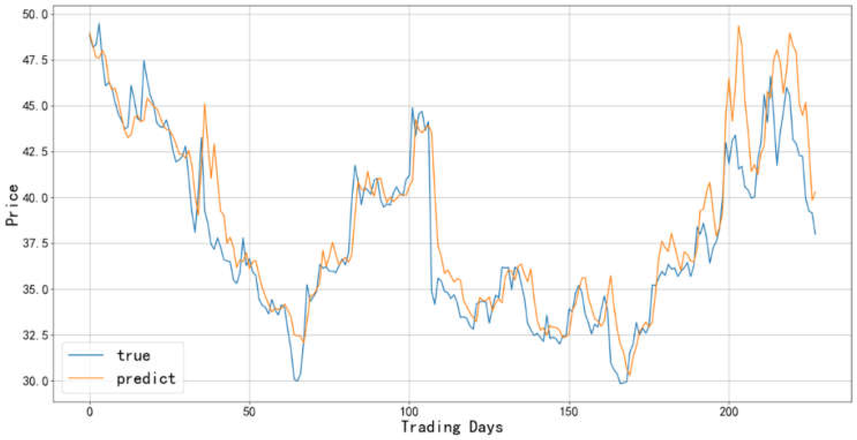
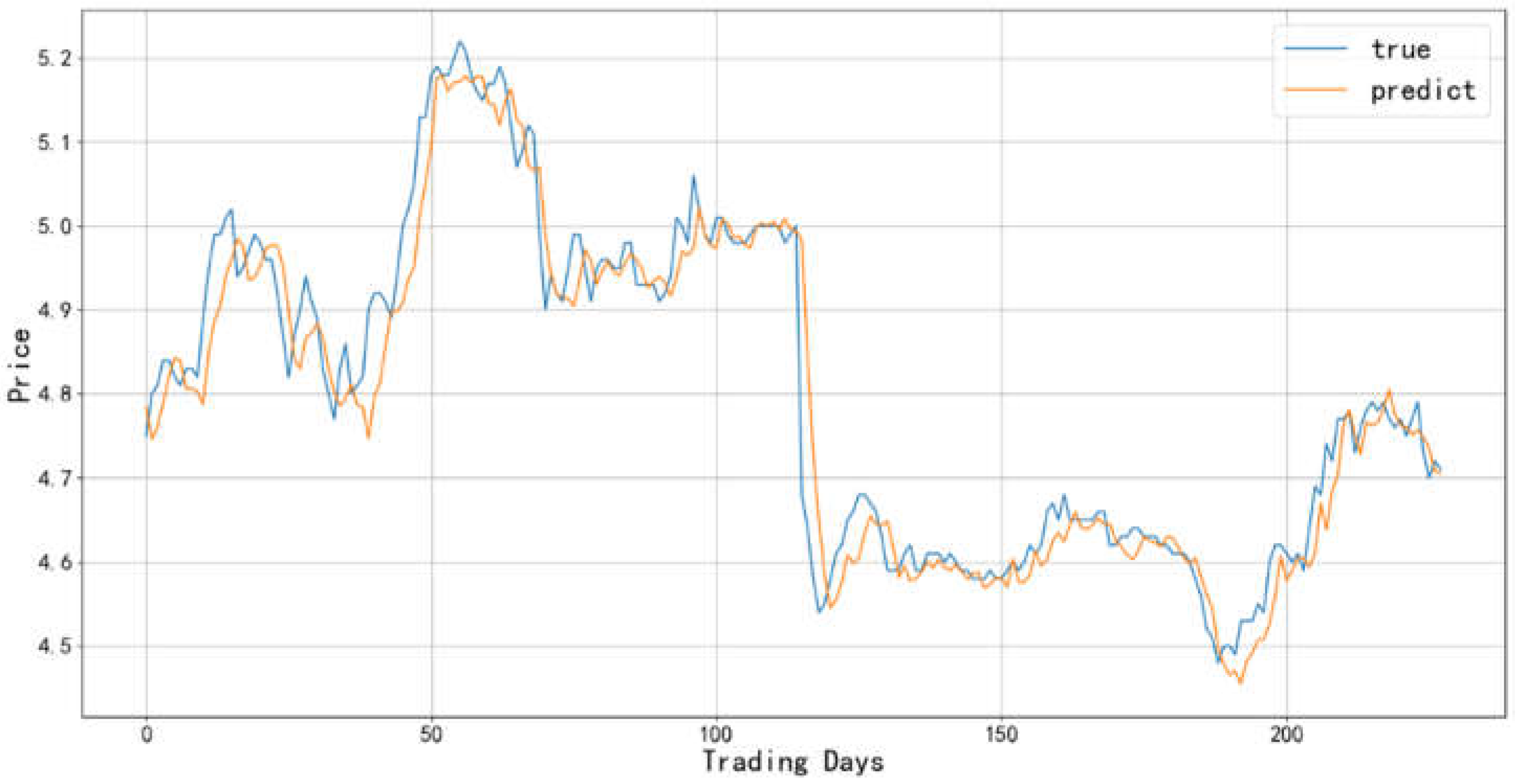
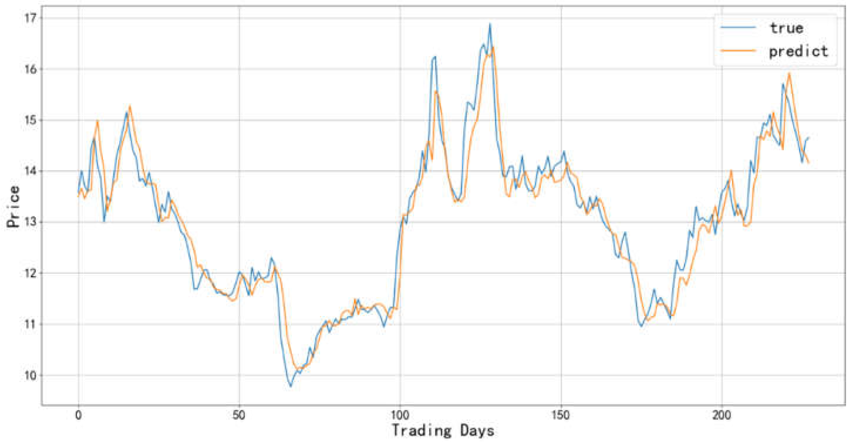
To visually illustrate the experimental results more effectively, Figure 8 present the loss function graphs of training and testing sets and Figure 9, Figure 10, Figure 11 and Figure 12 illustrate the trends of predicted and actual prices in the testing set for the four industries - Baijiu, Pharmaceutical Business, Bank, and Cinema Chain under the fixed selection method.
Figure 8. (a) Loss function error plot for Baijiu industry-1; (b) Loss function error plot for Pharmaceutical Business industry-1; (c) Loss function error plot for Bank industry-1; (d) Loss function error plot for Cinema Chain industry-1.
Preprints 78736 g008
Figure 9. Comparison between the predicted value and actual value of Baijiu industry-1
Preprints 78736 g009
Figure 10. Comparison between the predicted value and actual value of the Pharmaceutical Business industry-1
Preprints 78736 g010
Figure 11. Comparison between the predicted value and actual value of Bank industry-1
Preprints 78736 g011
Figure 12. Comparison between the predicted value and actual value of the Cinema Chain industry-1
Preprints 78736 g012

3.2. The experimental results of the Random selection method
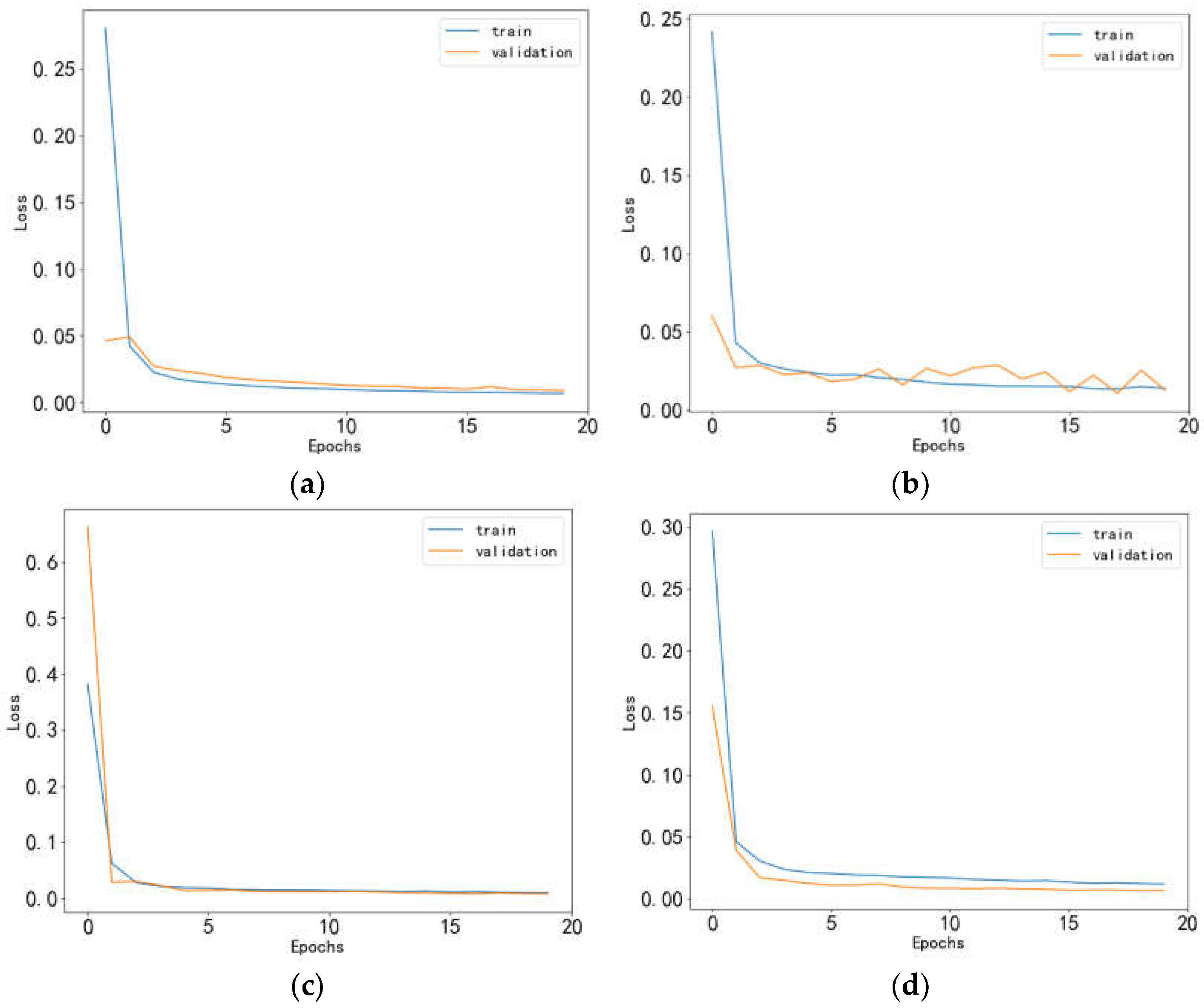
Figure 13 display the loss function graphs of training and testing sets and Figure 14, Figure 15, Figure 16 and Figure 17 display trends of predicted and actual prices in the testing set for the four industries - Baijiu, Pharmaceutical Business, Bank, and Cinema Chain under the fixed selection method.
Figure 13. (a) Loss function error plot for Baijiu industry-2; (b) Loss function error plot for Pharmaceutical Business industry-2; (c) Loss function error plot for Bank industry-2; (d) Loss function error plot for Cinema Chain industry-2.
Preprints 78736 g013
Figure 14. Comparison between the predicted value and actual value of Baijiu industry-2
Preprints 78736 g014
Figure 15. Comparison between the predicted value and actual value of the Pharmaceutical Business industry-2
Preprints 78736 g015
Figure 16. Comparison between the predicted value and actual value of Bank industry-2
Preprints 78736 g016
Figure 17. Comparison between the predicted value and actual value of the Cinema Chain industry-2
Preprints 78736 g017

3.3. Experimental Summary

Based on the experimental findings, it is evident that the stock prediction model proposed in this paper, along with the data reconstitution method, showcased a significant decrease in the loss function value across multiple industry-specific training and validation sets. Notably, even in the pharmaceutical business sector where slight fluctuations were observed, the performance of the model remained commendable. These results underscore the effectiveness of the experimental methodology in mitigating overfitting, thereby demonstrating its exceptional generalization capacity and robustness.

4. Discussion

This paper proposes a stock prediction model based on GRU with reconstructed datasets. Experimental results indicate that this approach significantly improves prediction accuracy, particularly across various industries. In contrast to previous studies that only modify the model using historical data from the target stock, this paper suggests incorporating data from other stocks within the industry sourced from the dataset itself. This enriches the features extracted by the model, reducing the risk of overfitting and improving prediction accuracy.
The auxiliary module in this model increases the amount of data, thereby expanding the training sample size and enhancing the training comprehensiveness, resulting in improved generalization capabilities. Moreover, different methods for selecting industry stocks yield varying degrees of accuracy improvement in the prediction. Random selection enables the acquisition of broader data features, leading to greater generalizability. , On the other hand, fixed selection provides more stable predictions but may limit the expression of the industry’s overall characteristics due to data selection constraints.
Therefore, this model, based on reconstructed datasets, offers a new perspective for stock prediction research and has positive implications for researchers and investors in the evaluation of stock value and risk assessment.

References

  1. Jin, Z., Yang, Y. and Liu, Y. Stock closing price prediction based on sentiment analysis and LSTM. Neural Computing and Applications 2019, 32(13): 1-17. [CrossRef]
  2. Box, G. E. P. and Pierce, D. A. Distribution of Residual Autocorrelations in Autoregressive-Integrated Moving Average Time Series Models. Journal of the American Statistical Association 2012, 65(332): 1509-1526.
  3. Press, D.; Orlando. Time Series Analysis: Forecasting and Control, Second Edition; Box, G. E. P., Jenkins, G. M.; Holden-Day, San Francisco, 1976; Volume 310, pp.144.
  4. Patel, J., Shah, S., Thakkar, P. and Kotecha, K. Predicting stock and stock price index movement using Trend Deterministic Data Preparation and machine learning techniques. Expert Systems with Applications 2015, 42(1): 259-268. [CrossRef]
  5. Chang, Y. H. and Lee, M. S. Incorporating Markov decision process on genetic algorithms to formulate trading strategies for stock markets. Applied Soft Computing 2017, 52: 1143-1153. [CrossRef]
  6. Dutta, S., Biswal, M. P., Acharya, S. and Mishra, R. Fuzzy stochastic price scenario based portfolio selection and its application to BSE using genetic algorithm. Applied Soft Computing 2018, 62: 867-891. [CrossRef]
  7. Patel, J., Shah, S., Thakkar, P. and Kotecha, K. Predicting stock market index using fusion of machine learning techniques. Expert Systems With Applications 2015, 42(4): 2162-2172. [CrossRef]
  8. Wu, W., Chen, W. and Liu, B. Using BP neural network to predict the rise and fall of the stock market (in Chinese). Dalian University of Technology Journal 2001, (01): 9-15.
  9. Ticknor, J. L. A Bayesian regularized artificial neural network for stock market forecasting. Expert Systems with Applications 2013, 40(14): 5501-5506. [CrossRef]
  10. Zhang, D. H. and Lou, S. The application research of neural network and BP algorithm in stock price pattern classification and prediction. Future Generation Computer Systems-the International Journal of Escience 2021, 115: 872-879. [CrossRef]
  11. Tay, F. E. H. and Cao, L. J. Application of support vector machines in financial time series forecasting. Omega-International Journal of Management Science 2001, 29(4): 309-317. [CrossRef]
  12. Kim, K.-j. Financial time series forecasting using support vector machines. Neurocomputing 2003, 55(1): 307-319. [CrossRef]
  13. Ran, Y. and Jiang, H. Stock Prices Prediction based on Back Propagation Neural Network and Support Vector Regression (in Chinese). Journal of Shanxi University. Natural Science Edition 2018, 41(1): 1-14. [CrossRef]
  14. Hinton, G. E. and Salakhutdinov, R. R. Reducing the Dimensionality of Data with Neural Networks. Science 2006, 313(5786): 504-507.
  15. Singh, R. and Srivastava, S. Stock prediction using deep learning. Multimedia Tools and Applications 2017, 76(18): 18569-18584.
  16. Luca, D. P. and Oleksandr, H. Artificial neural networks architectures for stock price prediction: Comparisons and applications. International Journal of Circuits, Systems and Signal Processing 2016, 10: 403-413.
  17. Kraus, M. and Feuerriegel, S. Decision support from financial disclosures with deep neural networks and transfer learning. Decision Support Systems 2017, 104: 38-48. [CrossRef]
  18. Chong, E., Han, C. and Park, F. C. Deep learning networks for stock market analysis and prediction: Methodology, data representations, and case studies. Expert Systems with Applications 2017, 83: 187-205. [CrossRef]
  19. Cui, D.; A Study on the Prediction of Stock Price based Deep Belief Networks (in Chinese). Master’s degree, Huazhong University of Science and Technology, Wuhan, 2016.
  20. Liu, Q.; Short term stock price forecasting based on fuzzy deep learning network algorithm (in Chinese). Master’s degree, Harbin Institute of Technology, Harbin,2016.
  21. Li, X. M.; Yang, L.; Xue, F. Z.; Zhou, H. J. Time series prediction of stock price using deep belief networks with Intrinsic Plasticity. 29th Chinese Control and Decision Conference (CCDC), Chongqing, CHINA, 28-30 May 2017. [CrossRef]
  22. Tsantekidis, A.; Passalis, N.; Tefas, A.; Kanniainen, J.; Gabbouj, M.; Iosifidis, A. Forecasting Stock Prices from the Limit Order Book using Convolutional Neural Networks. IEEE 19th Conference on Business Informatics CBI, Thessalonki, GREECE, Jul 24-26 Jul 2017.
  23. Hsieh, T. J., Hsiao, H. F. and Yeh, W. C. Forecasting stock markets using wavelet transforms and recurrent neural networks: An integrated system based on artificial bee colony algorithm. Applied Soft Computing 2011, 11(2): 2510-2525. [CrossRef]
  24. Rather, A. M., Agarvval, A. and Sastry, V. N. Recurrent neural network and a hybrid model for prediction of stock returns. Expert Systems with Applications 2015, 42(6): 3234-3241. [CrossRef]
  25. Qin, Y.; Song, D. J.; Cheng, H. F.; Cheng, W.; Jiang, G. F.; Cottrell, G. W. A Dual-Stage Attention-Based Recurrent Neural Network for Time Series Prediction. 26th International Joint Conference on Artificial Intelligence (IJCAI), Melbourne, AUSTRALIA, 19-25 Aug 2017. [CrossRef]
  26. Sim, H. S., Kim, H. I. and Ahn, J. J. Is Deep Learning for Image Recognition Applicable to Stock Market Prediction? Complexity 2019: 10.
  27. Chen, W., Jiang, M. R., Zhang, W. G. and Chen, Z. S. A novel graph convolutional feature based convolutional neural network for stock trend prediction. Information Sciences 2021, 556: 67-94. [CrossRef]
  28. Hochreiter, S. and Schmidhuber, J. Long short-term memory. Neural Computation 1997, 9(8): 1735-1780.
  29. Yang, Q. and Wang, C. A Study on Forecast of Global Stock Indices Based on Deep LSTM Neural Network (in Chinese). Statistical Research 2019, 36(03): 65-77.
  30. Lee, M. C. Using support vector machine with a hybrid feature selection method to the stock trend prediction. Expert Systems with Applications 2009, 36(8): 10896-10904. [CrossRef]
  31. Teng, X., Wang, T., Zhang, X., Lan, L. and Luo, Z. G. Enhancing Stock Price Trend Prediction via a Time-Sensitive Data Augmentation Method. Complexity 2020, 2020: 8. [CrossRef]
Disclaimer/Publisher’s Note: The statements, opinions and data contained in all publications are solely those of the individual author(s) and contributor(s) and not of MDPI and/or the editor(s). MDPI and/or the editor(s) disclaim responsibility for any injury to people or property resulting from any ideas, methods, instructions or products referred to in the content.
Copyright: This open access article is published under a Creative Commons CC BY 4.0 license, which permit the free download, distribution, and reuse, provided that the author and preprint are cited in any reuse.
Prerpints.org logo

Preprints.org is a free preprint server supported by MDPI in Basel, Switzerland.

Subscribe

© 2024 MDPI (Basel, Switzerland) unless otherwise stated