You are currently viewing a beta version of our website. If you spot anything unusual, kindly let us know.

Preprint

Article

On the Interpolation Error Distribution in Collocation Comparison of Atmospheric Profiles

Altmetrics

Downloads

110

Views

Comments

A peer-reviewed article of this preprint also exists.

This version is not peer-reviewed

Abstract

The intercomparison among different atmospheric monitoring systems is key for instrument calibration and validation. Common cases involve satellites, radiosonde, radio occultation (e.g. GNSS-RO) and atmospheric model outputs (e.g. ERA5 reanalysis). Since instruments and/or measures are not perfectly collocated, the miss-collocation uncertainty must be considered in the related intercomparison uncertainty budgets.

Keywords:

Subject: Environmental and Earth Sciences - Atmospheric Science and Meteorology

1. Introduction

Nowadays, along with atmospheric parameters measured at a fixed point in space, an array of meteorological quantities (e.g., wind speed and direction, temperature, pressure, humidity, atmospheric composition, etc.) are acquired as vertical profiles describing the physical properties of a column of air varying with altitude. This is made possible by major technological advances over the past few decades regarding atmospheric sensors as well as sensor platforms. In high-resolution (≈1 m) applications, traditional instruments such as tethersondes, radiosondes, and dropsondes are used for vertical profiling [1]. However, to a certain extent (although at relatively coarse vertical resolution), these in-situ measurements can be complemented with different remote sensing techniques using ground-based (e.g., lidars and microwave radiometers) and satellite-born instruments.

Investigating the vertical structure of the atmosphere by satellite instruments dates from the 1970s [2]. The first publications on intercomparisons of satellite and radiosonde profiles proved the capability of the new technique [3,4,5,6], which has largely compensated for the limitation of coverage over land and oceans by balloon-born measurements [7]. Most notably, the datasets of temperature, humidity and pressure, available through Global Navigation Satellite System Radio Occultations (GNSS-RO) [8,9] since the early 2000s and serving as the main input for numerical weather predictions (NWPs), are reliable data sources supporting climate change assessments [10].

Although having a relatively coarse horizontal resolution (∼300−400 km), the effective vertical resolution of GNSS-RO measurements below 15 km altitude is from 100 m to 300 m [11], which is suitable for resolving relatively small-scale atmospheric variability in vertical dimension [12,13,14]. In addition, hyperspectral infrared sounders such as the Atmospheric Infrared Sounder (AIRS) onboard NASA’s Aqua satellite and the Infrared Atmospheric Sounding Interferometers (IASIs) on the EUMETSAT MetOp satellites have become valuable data sources for a wide range of applications [15,16,17]. Although having some known limitations [12,18,19,20,21,22], GNSS-RO, AIRS and IASI measurements are now assimilated into operational NWP models and different reanalyses, which allow investigating the state of the atmosphere in a three-dimensional grid of points [10]. Either an operative NWP or reanalysis, the final product is a gridded representation of a geophysical quantity based on irregularly spaced observations. For example, ERA5 – assessed as the most reliable reanalysis for climate trend evaluation – provides hourly fields available at a horizontal resolution of 31 km on 37 pressure levels, from the surface up to 1 hPa [10,23]. According to the standard atmosphere, the vertical resolution of ERA5 is <250 m at the lowest levels up to 1 km at tropopause height.

With the diversity of atmospheric sounding techniques, new challenges come for establishing reference methods. This, in turn, requires assessing instrumental performance and quantifying the biases and uncertainties. Such extensive knowledge is derived from laboratory tests and intercomparisons, the latter being a common practice and a requirement for improving the global climate observing system [24,25,26]. An intercomparison aims to determine whether different observing systems agree within their known limitations [27].

Comparison of atmospheric profiles derived from two or more instruments must consider the spatial displacement of the measurements. Generally, the instruments included in the analysis are relatively close to each other but usually not measured at the same point in space and time (not the case for twin radiosoundings, where different instruments are fixed to the same ascending balloon). Typically, an assumption is made that within a few hours and some tens of kilometres in horizontal displacement, the properties of the atmosphere do not vary significantly, allowing for the comparison of two ground-based soundings within these limits without any horizontal and temporal interpolation [28]. However, the criteria for comparing ground-based sounding with a satellite-born counterpart is less strict to increase the number of satellite profiles suitable for co-location, the latter directly depending on the position of the satellite(s). Then, the horizontal and temporal mismatch limits used in earlier publications reach up to several hundreds of kilometres and 7 hours, respectively [29,30,31,32,33,34,35].

On the other hand, vertical mismatch of levels used in co-located profiles is often addressed through interpolation of a profile with a higher vertical resolution (e.g., radiosonde) to the pressure levels of another profile with a lower resolution (e.g., satellite product). For example, the GNSS-RO observations are defined along a vertical grid (60 levels in the case of GNSS-RO products [29,36]), which does not coincide with the irregular grid of the in-situ profiles (several thousand in the case of raw radiosonde data). Therefore, the co-located profiles of radiosonde are usually interpolated to the vertical levels of the GNSS-RO. Similar interpolation is inevitable while comparing instruments with NWP models. For example, the IASI temperatures are given at 90 pressure levels (version 4 and 5 temperature profiles) or at 101 pressure levels (version 6 temperature profiles). For comparing the profiles with ERA5, the IASI temperature profiles are interpolated to the ERA5 pressure levels [17]. This step introduces an interpolation uncertainty component that must be considered in the total co-location uncertainty budget, including instrumental uncertainty and components from horizontal and temporal mismatch [37,38].

It must be noted that intercomparisons can also be carried out between different numerical models [39,40] and radiosonde types [41,42], between an instrument and any other type of instruments suitable for measuring the same parameters in the same atmospheric conditions [43]. In the case of intercomparisons including a three-dimensional model, an additional horizontal interpolation of model data to the locations of the data points from the instrument is applied [17,40].

This article is motivated by the comparison of GNSS-RO temperature with ERA5 outputs. We notice that both GNSS-RO retrievals and ERA5 model outputs are spatially and temporally smoothed, as discussed above. Hence, to separate interpolation uncertainty from the other collocation uncertainty sources, we consider reference measurements at ERA5 levels with high quality and high resolution. In fact, we use reference measurements given by GRUAN Data Processing (GDP) for Vaisala RS41 radiosonde [44], which are available at both the GNSS-RO and ERA5 pressure levels, with, say, a 1 s accuracy.

The paper provides a novel interpolation algorithm based on a state space representation (e.g., [45]), which has a performance equivalent to linear interpolation but provides an estimate of the interpolation uncertainty.

The new algorithm and linear interpolation are tested in interpolating the 37 ERA5 pressure levels starting from the 60 GNSS-RO levels. We compare the interpolated values with the true ones and assess the related interpolation uncertainty by latitude, altitude, season and time of the day.

An important by-product is the study of the interpolation error distribution, which is shown to be non-Gaussian. A scaled Student’s t distribution adapts well to our data. Due to this result, using a coverage factor k=2 in Immler’s inequality [24] is questioned, and an alternative is provided.

2. Materials and Methods

2.1. Data

The current analysis considers collocated GRUAN-processed radiosonde (RS41-GDP1, [46,47],) and GNSS-RO measurements from the Metop satellite collected during 2020. The Metop atmospheric profile data were obtained from the publicly available archive of the Radio Occultation Meteorology Satellite Application Facility; see the Data Availability Statement below. A horizontal distance of 300 km and a time difference of 3 h are used as collocation criteria. The data were categorized by time of day based on the solar elevation angle (SEA), which depends on time, latitude, and longitude. The SEA ranges for "day," "night," and "dusk//dawn" data were 7.5 to 90, −90 to −7.5, and −7.5 to 7.5 degrees, respectively. The season was determined based on the latitude and month to consider the seasonal differences between the southern and northern hemispheres. The data included in this study are summarised in Table 1.

The data set is seasonally balanced for all stations but Ross Island, which has approximately one-half in summer and fall of the observations in winter and spring; see Table 2. Considering the time of the day, some stations are strongly unbalanced with only two or three profiles in dusk/dawn or night; see Table 3. This will be considered in the subsequent analysis.

2.2. Interpolation by State Space models

In this section, we introduce a statistical model based on the well-known class of State Space models [45] propagating the measurement uncertainty to interpolated points while taking into account interpolation uncertainty.

Let

y_{i}

denote the observation of the geophysical quantity of interest, e.g., Temperature [K], at pressure level

p_{i}

i = 1, . . ., n

where n is the number of observations of the profile under consideration. We assume a measurement equation error for

y_{i}

given by

y_{i} = x_{i} + ε_{i} .

(1)

Here,

x_{i}

is the "true" state and

ε_{i}

is the random measurement error with uncertainty

u_{i} = \sqrt{V a r (ε_{i})}

where

V a r ()

is the variance operator. For the state x, we assume locally linear dynamics with respect to pressure, given by

\begin{matrix} x_{i} & = & x_{i - 1} + α_{i} \times (p_{i} - p_{i - 1}) + η_{x, i} \end{matrix}

(2)

\begin{matrix} α_{i} & = & α_{i - 1} + η_{α, i} \end{matrix}

(3)

where

η_{x, i}

and

η_{α, i}

are independent innovation processes with zero mean and variance

σ_{x}^{2}

and

σ_{α}^{2}

respectively. Equation 2 states that apart from the stochastic component

η_{x}

, the geophysical state has a local linear variation with respect to the pressure levels. Equation 3 implies a smooth variation of the coefficient

α

For any pressure level

p^{*} \in [p_{i}, p_{i - 1}]

the optimal estimate of the corresponding state

x^{*}

is given by the following conditional expectation

{\hat{x}}^{*} = E (x^{*} | y_{1}, \dots, y_{n})

(4)

which is readily computed by the Kalman smoother (KS) algorithm under Gaussian assumptions [rif]. In addition, the uncertainty at

p^{*}

is given by

u_{K S} {({\hat{x}}^{*})}^{2} = V a r (x^{*} | y_{1}, \dots, y_{n})

(5)

which also is an output of the above-mentioned KS algorithm.

2.3. Interpolation errors and uncertainty

For each single profile, let us denote by

(y_{i}, p_{i}), i = 1, \dots, n

the observations at GNSS-RO levels, and by

(y_{j}^{*}, p_{j}^{*}), i = 1, \dots, n^{*}

the true values at ERA5 levels. Let

{\hat{y}}_{L I N T, j}

and

{\hat{y}}_{K S, j}

be the linear and Kalman smoother interpolations at ERA5 levels, respectively, and let

e_{L I N T, j}

and

e_{K S, j}

be the corresponding interpolation errors, e.g.

e_{L I N T, j} = {\hat{y}}_{L I N T, j} - y_{j}^{*}

. In the sequel, we focus on altitudes below 10 hPa. As a result, we have

n^{*} = 31

ERA5 levels, and

n \leq 46

GNSS-RO levels, depending on missing data, the average being

n = 44

"Observed" interpolation uncertainty is computed using root mean square error (RMSE) and mean absolute error (MAE). Consider a subset of all profiles, e.g. a station or a season, and denote it by

S

, with profile identifiers

i d \in S

. For methods

m = L I N T, K S

, we have

R M S E_{m, S} = \sqrt{\frac{1}{n^{*} | | S | |} \sum_{j \leq n^{*}, i d \in S} e_{m, i d, j}^{2}}

and

M A E_{m, S} = \sqrt{\frac{1}{n^{*} | | S | |} \sum_{j \leq n^{*}, i d \in S} | | e_{m, i d, j} | |} .

It is well known that RMSE, being a quadratic metric, is suited for Gaussian errors but is prone to outliers and high tails. Instead, MAE is a robust metric suitable for outliers resistance and high tails.

2.4. Non-Gaussian errors

In collocation comparisons, two measurements

m_{1}

and

m_{2}

, with uncertainties

u_{1}

and

u_{2}

, are said to be in agreement [24] if the error

e = m_{1} - m_{2}

, is small, namely

| e | < k \times u_{e}

(6)

for

k = 2

. In this formula,

u_{e}

is the collocation uncertainty. If the uncertainties are uncorrelated and no collocation mismatch affects the measurements, then

u_{e} = \sqrt{u_{1}^{2} + u_{2}^{2}}

. It is well known that

k = 2 (3)

has the interpretation of a statistical test with false rejection probability

α ≅ 5 % (0.27 %)

if e is Gaussian distributed.

If the error distribution has higher tails than the Gaussian distribution, the interpretation of k may be different. Considering a scaled Student’s t distribution, with

ν > 4

degrees of freedom and scale parameter

u_{e} = \sqrt{v a r (e)}

, it is worth noting that the 97.5% percentile is close to the corresponding Gaussian percentile, namely 1.96, for any

ν > 4

. Instead, the probability of large errors, related to

k \geq 3

, for the mentioned t distribution is much larger than the Gaussian counterpart, even if the two measurements come from the same instrument. See some examples in Table 4.

2.5. Inference for the Student’s t distribution

Our case study found that errors have kurtosis, say

k (e)

, well above the Gaussian value of three. In fact, the KS error distribution, shown in Figure 1 and Figure 2, has the typical behaviour of a large t-distributed dataset with little degrees of freedom.

It is interesting to note that the Student’s t distribution may be seen as the compound of the Gaussian distribution with variance given by an inverse Gamma random variable. This evidence could bring us to extend the Gaussian State Space model of Section 2.2. Recently, Kalman filters have been developed using the Student’s t distribution for the measurement error in Equation 1, see, e.g. [48]. In our case, we have a sampling issue since, apart from the testing case on GRUAN data, we do not have the availability of measurements on ERA5 levels. As a result, the RMSE on ERA5 levels is much larger than that on GNSS-RO levels.

For this reason, we postpone the full non-Gaussian State Space model to further research. Instead, in this paper, we use a two-step approach. First, we compute Linear and (Gaussian) KS interpolation. Second, we fit the errors by a scaled t distribution with degrees of freedom parameter, say

ν

, and standard error

σ

, depending on the data. This approach allows us to better understand the uncertainty of the data at hand.

In particular, the

ν > 4

parameter is estimated by the method of moments, say

\hat{ν} = 4 + \frac{6}{k (e) - 3}

. Then, the scale

σ

parameter is estimated by the plug-in maximum likelihood method, say

\hat{σ} = {\hat{σ}}_{\hat{ν}}

. Since the sample sizes are large, we do not mind about the loss in efficiency related to the method of moments.

3. Results

Using data from Table 1 and methods detailed in the previous section, we computed linear and KS interpolation and the related errors at ERA5 levels. The first important result is that the errors of the two methods are equivalent. In fact, the mean difference is quite small,

\bar{e_{L} - e_{K}} = 0.004 K

, the Spearman correlation coefficient is quite large

r (e_{L}, e_{K}) > 0.95

, and

R M S E (e_{L}, e_{K}) = 0.14 K

. Hence in the sequel, we focus on KS results and omit the subscript K wherever clear.

In this section, we assess the interpolation uncertainty by latitude, altitude, season and time of the day. In particular, we consider the RMSE, which, for different reasons, may be prone to outliers and non-Gaussianity. Also, we consider the robust metrics given by MAE and Student’s t standard error,

σ

3.1. Uncertainty by station

Since the GRUAN stations used are located in various continents and at latitudes spanning from +78° to −78° an important question is related to the geographical stability of interpolation uncertainty.

Table 5 reports various uncertainty measures by station. As a reference, we give the median of the measurement uncertainty reported by the GDP and the interpolation uncertainty given by KS. We also report the RMSE, MAE, Student’s t scale and degrees of freedom parameters for the KS interpolation errors. The standard errors of these uncertainties measures and t-distribution parameters are very small, as shown in Table 6.

It may be noticed from the last column of Table 5 that the tail parameter

\hat{ν}

is essentially constant along the stations. Considering interpolation uncertainty, the tropic station of Singapore has the highest interpolation uncertainty metrics even if the GDP uncertainty is not. The antarctic station of Ross Island has the lowest metrics even if the GDP uncertainty is higher. The northern stations have similar interpolation metrics, even if Lindenberg has a considerably lower GDP uncertainty.

From these figures, it is seen that the interpolation uncertainty is more influenced by atmospheric dynamics than the measurement uncertainty. It is also interesting to observe the overestimation of the uncertainty provided by the RMSE due to its sensitivity to large errors. Once the high tails are taken into account using the t-distribution approach, the maximum likelihood estimate of the uncertainty, namely

\hat{σ}

, is quite smaller than RMSE and close to the robust metric given by MAE.

3.2. Uncertainty by altitude

Figure 3 depicts the vertical behaviour of interpolation uncertainty assessed by MAE and compared to the median of measurement uncertainty, u, and KS uncertainty,

u_{K S}

, as in Equation (5). Similarly, Figure 4 describes the RMSE behaviour and compares it to the quadratic means of u and

u_{K S}

It may be noted that both MAE and RMSE interpolation uncertainties are close to the measurement uncertainty below the tropopause, with

M A E < 0.2

K. Instead, around 300 hPa, both show an increase and an even steeper increase above that, with

M A E

near 0.8 K above 100 hPa. Additional insight is provided by Figure 5, which depicts the vertical profile of MAE by station. It is clearly seen that the equatorial station of Singapore has the larger uncertainty in the upper atmosphere. After excluding this, the other stations agree with the above uncertainty limit of 0.8 K above 250 hPa. In particular, the Antarctic station of Ross Island has the smallest interpolation uncertainty in the upper atmosphere.

It is interesting to note that the interpolation uncertainty may be smaller than the measurement uncertainty. This is consistent with the fact that the temperature profile may be very smooth, and using neighbouring observations may improve the measurement precision. Comparing the blue and green lines of Figure 3 and Figure 4, we see that KS and LINT are quite similar, but, at the tropopause, near 300 hPa, KS provides better interpolation.

The KS interpolation uncertainty (

u_{K S}

) is larger than RMSE and/or MAE below 200 hPa and smaller above. For operational use of

u_{K S}

, we suggest the correction given by Equation (15) of [37].

3.3. Uncertainty by season

After observing the uncertainty sensitivity to latitude in Section 3.1, we test for similar seasonal effects in this section. Reading Table 7 from right to left and considering the related standard errors reported in Table 8, we see that the t-distribution parameters

ν

and

σ

are quite close for the different seasons. The minimum interpolation uncertainty (either RMSE, MAE or

σ

) is observed in summer with a difference of 0.01−0.02 K with respect to the overall quantity. Again, we have little uncertainty variation among seasons.

3.4. Uncertainty by time of the day

Table 9 and Table 10 report the interpolation uncertainty metrics and their standard errors classified by time of the day for the entire data set and for the Lindenberg data alone. It is seen that during dusk/dawn, the overall interpolation error distribution has higher tails, with lower degrees of freedom

ν

and a higher RMSE, exceeding by about 0.03 K the day and night counterparts. This is not the case for Lindenberg data. To have further insight, Table 11 and Table 12 provide MAE and RMSE by station and time of the day. It is again clear that the variation of uncertainty is led more by geography rather than by time of the day. Notice that Singapore shows a reduction in the nighttime, but the standard error is higher due to the small profile number for this case, as mentioned in Section 2.1 and highlighted in Table 3.

4. Discussion and conclusions

The interpolation of temperature at ERA5 levels using data on GNSS-RO levels results in error distributions with tails higher than the Gaussian distribution. The analysis based on GRUAN-processed radiosonde data shows that, in general, a t-distribution with about

ν = 4.3

degrees of freedom is appropriate. We suggest using MAE and/or

σ

to assess such a non-Gaussian uncertainty. Comparing them to RMSE helps to highlight the high tail impact on uncertainty.

The overall uncertainty of temperature profiles is about 0.25 K for MAE and t-distribution scale parameter

σ

. Instead, it is about 0.5 K for RMSE. Such figures are mainly influenced by latitude and geography, with higher values in the tropics and smaller ones near the poles. In particular, Ross Island station at −78° Latitude gives uncertainties which are smaller than Ny-Alesund station at +78° Latitude. This effect is more evident in the higher atmosphere, above 300 hPa, where MAE increases up to 0.8 K for most stations except for the equatorial station of Singapore, where a discernible increase in the degree of interpolation uncertainty within the upper troposphere/lower stratosphere is revealed, exceeding 1 K. On the opposite, Ross Island has the smallest uncertainty at these altitudes. The findings regarding temperature uncertainty dependence on latitude are consistent with previous research that has observed a pronounced change in temperature lapse rate within the specified altitude range in the tropics [19]. When the lapse rate undergoes rapid changes with altitude, it becomes increasingly difficult to estimate temperatures accurately through interpolation. In such cases, larger interpolation errors become inevitable.

It may be noted that the horizontal and vertical variations dominate the temporal sources of variation considered. Namely, season and time of the day, which can be ignored in this respect.

We considered both linear interpolation and interpolation based on Kalman smoother. The two methods resulted very close in terms of performance, but KS is slightly better near the tropopause. In addition, KS provides interpolation uncertainties for individual profiles, which may be useful in practice.

As a final remark, the KS interpolation uncertainty is often smaller than the measurement uncertainty. This is due to the smoothness of the temperature profiles, so using neighbouring information improves the understanding of the temperature state.

Author Contributions

Conceptualization, AF, HK and KR; methodology, AF; software, AF and HK; validation, AF; data analysis, AF and HK; statistical modelling, AF; data curation, HK; writing—original draft preparation, AF, HK and KR; writing—review and editing, AF, HK and KR; visualization, AF. All authors have read and agreed to the published version of the manuscript.

Funding

This research received no external funding

Data Availability Statement

GRUAN data are available at https://www.gruan.org/data/file-archive/rs41-gdp1-at-lc; registration is required for downloading the data sets. GNSS-RO measurements from the Metop satellite can be obtained from the publicly available archives of the Radio Occultation Meteorology Satellite Application Facility [36]; registration is required for downloading the data sets.

Acknowledgments

We wish the express our sincere thanks to GRUAN Lead Center and especially to Michael Sommer for the help and guidance in getting the data and in the release interpretation.

Conflicts of Interest

The authors declare no conflict of interest.

References

Tropea, C.; Yarin, A.L.; Foss, J.F.; others. In Springer handbook of experimental fluid mechanics; Springer, 2007; Vol. 1.
Thompson, O.E.; Eom, J.K.; Wagenhofer, J.R. On the resolution of temperature profile finestructure by the NOAA satellite vertical temperature profile radiometer. Monthly Weather Review 1976, 104, 117–126. [Google Scholar] [CrossRef]
Smith, W.L.; Woolf, H. An intercomparison of meteorological parameters derived from radiosonde and satellite vertical temperature cross sections; Vol. 55, National Environmental Satellite Service, 1974. [Google Scholar]
Shen, W.C.; Smith, W.L.; Woolf, H. An intercomparison of radiosonde and satellite-derived cross sections during the AMTEX; Number 72, National Environmental Satellite Service, 1975. [Google Scholar]
Horn, L.H.; Petersen, R.A.; Whittaker, T.M. Intercomparisons of data derived from Nimbus 5 temperature profiles, rawinsonde observations and initialized LFM model fields. Monthly Weather Review 1976, 104, 1362–1371. [Google Scholar] [CrossRef]
Hilsenrath, E.; Coley, R.; Kirschner, P.; Gammill, B. A rocket ozonesonde for geophysical research and satellite intercomparison. Technical report, 1979.
Trenberth, K.; Jones, P.; Ambenje, P.; Bojariu, R.; Easterling, D.; Klein Tank, A.; Parker, D.; Rahimzadeh, F.; Renwick, J.; Rusticucci, M. others. Chapter 3. Observations: surface and atmospheric climate change. In Climate Change 2007: the physical science basis. Contribution of Working Group I to the fourth assessment report of the Intergovernmental Panel on Climate Change; (Eds S Solomon, D Qin, M Manning, Z Chen, M Marquis, KB Averyt, M Tignor, HL Miller), 2007; pp. 235–336. [Google Scholar]
Foelsche, U.; Scherllin-Pirscher, B.; Ladstädter, F.; Steiner, A.; Kirchengast, G. Refractivity and temperature climate records from multiple radio occultation satellites consistent within 0.05%. Atmospheric Measurement Techniques 2011, 4, 2007–2018. [Google Scholar] [CrossRef]
Anthes, R. Exploring Earth’s atmosphere with radio occultation: contributions to weather, climate and space weather. Atmospheric Measurement Techniques 2011, 4, 1077–1103. [Google Scholar] [CrossRef]
Chen, D.; Rojas, M.; Samset, B.; Cobb, K.; Diongue Niang, A.; Edwards, P.; Emori, S.; Faria, S.; Hawkins, E.; Hope, P.; others. Framing, context, and methods. Climate change 2021, 478, 147–286. [Google Scholar]
Zeng, Z.; Sokolovskiy, S.; Schreiner, W.S.; Hunt, D. Representation of vertical atmospheric structures by radio occultation observations in the upper troposphere and lower stratosphere: Comparison to high-resolution radiosonde profiles. Journal of Atmospheric and Oceanic Technology 2019, 36, 655–670. [Google Scholar] [CrossRef]
Scherllin-Pirscher, B.; Steiner, A.K.; Kirchengast, G.; Schwärz, M.; Leroy, S.S. The power of vertical geolocation of atmospheric profiles from GNSS radio occultation. Journal of Geophysical research: atmospheres 2017, 122, 1595–1616. [Google Scholar] [CrossRef] [PubMed]
Wilhelmsen, H.; Ladstädter, F.; Scherllin-Pirscher, B.; Steiner, A.K. Atmospheric QBO and ENSO indices with high vertical resolution from GNSS radio occultation temperature measurements. Atmospheric Measurement Techniques 2018, 11, 1333–1346. [Google Scholar] [CrossRef]
Stocker, M.; Ladstädter, F.; Wilhelmsen, H.; Steiner, A.K. Quantifying Stratospheric Temperature Signals and Climate Imprints From Post-2000 Volcanic Eruptions. Geophysical Research Letters 2019, 46, 12486–12494. [Google Scholar] [CrossRef] [PubMed]
Chahine, M.T.; Pagano, T.S.; Aumann, H.H.; Atlas, R.; Barnet, C.; Blaisdell, J.; Chen, L.; Divakarla, M.; Fetzer, E.J.; Goldberg, M.; others. AIRS: Improving weather forecasting and providing new data on greenhouse gases. Bulletin of the American Meteorological Society 2006, 87, 911–926. [Google Scholar] [CrossRef]
Hilton, F.; Atkinson, N.; English, S.; Eyre, J. Assimilation of IASI at the Met Office and assessment of its impact through observing system experiments. Quarterly Journal of the Royal Meteorological Society: A journal of the atmospheric sciences, applied meteorology and physical oceanography 2009, 135, 495–505. [Google Scholar] [CrossRef]
Bouillon, M.; Safieddine, S.; Hadji-Lazaro, J.; Whitburn, S.; Clarisse, L.; Doutriaux-Boucher, M.; Coppens, D.; August, T.; Jacquette, E.; Clerbaux, C. Ten-year assessment of IASI radiance and temperature. Remote Sensing 2020, 12, 2393. [Google Scholar] [CrossRef]
Angerer, B.; Ladstädter, F.; Scherllin-Pirscher, B.; Schwärz, M.; Steiner, A.K.; Foelsche, U.; Kirchengast, G. Quality aspects of the Wegener Center multi-satellite GPS radio occultation record OPSv5. 6. Atmospheric Measurement Techniques 2017, 10, 4845–4863. [Google Scholar] [CrossRef]
Gleisner, H.; Lauritsen, K.B.; Nielsen, J.K.; Syndergaard, S. Evaluation of the 15-year ROM SAF monthly mean GPS radio occultation climate data record. Atmospheric Measurement Techniques 2020, 13, 3081–3098. [Google Scholar] [CrossRef]
Steiner, A.K.; Ladstädter, F.; Ao, C.O.; Gleisner, H.; Ho, S.P.; Hunt, D.; Schmidt, T.; Foelsche, U.; Kirchengast, G.; Kuo, Y.H.; others. Consistency and structural uncertainty of multi-mission GPS radio occultation records. Atmospheric Measurement Techniques 2020, 13, 2547–2575. [Google Scholar] [CrossRef]
Blackwell, W.; Milstein, A. A neural network retrieval technique for high-resolution profiling of cloudy atmospheres. IEEE Journal of Selected Topics in Applied Earth Observations and Remote Sensing 2014, 7, 1260–1270. [Google Scholar] [CrossRef]
Susskind, J.; Blaisdell, J.M.; Iredell, L. Improved methodology for surface and atmospheric soundings, error estimates, and quality control procedures: the atmospheric infrared sounder science team version-6 retrieval algorithm. Journal of Applied Remote Sensing 2014, 8, 084994–084994. [Google Scholar] [CrossRef]
Hersbach, H.; Bell, B.; Berrisford, P.; Hirahara, S.; Horányi, A.; Muñoz-Sabater, J.; Nicolas, J.; Peubey, C.; Radu, R.; Schepers, D.; others. The ERA5 global reanalysis. Quarterly Journal of the Royal Meteorological Society 2020, 146, 1999–2049. [Google Scholar] [CrossRef]
Immler, F.; Dykema, J.; Gardiner, T.; Whiteman, D.; Thorne, P.; Vömel, H. Reference quality upper-air measurements: Guidance for developing GRUAN data products. Atmospheric Measurement Techniques 2010, 3, 1217–1231. [Google Scholar] [CrossRef]
Zhongming, Z.; Linong, L.; Xiaona, Y.; Wangqiang, Z.; Wei, L. ; others. Systematic Observation Requirements for Satellite-based Products for Climate Supplemental details to the satellite-based component of the Implementation Plan for the Global Observing System for Climate in Support of the UNFCCC: 2011 update 2011.
Zemp, M.; Chao, Q.; Han Dolman, A.J.; Herold, M.; Krug, T.; Speich, S.; Suda, K.; Thorne, P.; Yu, W. GCOS 2022 Implementation Plan. Global Climate Observing System GCOS.
Rodgers, C.D. Inverse methods for atmospheric sounding: theory and practice. Vol. 2, World scientific, 2000. [Google Scholar]
Weaver, D.; Strong, K.; Schneider, M.; Rowe, P.M.; Sioris, C.; Walker, K.A.; Mariani, Z.; Uttal, T.; McElroy, C.T.; Vömel, H.; others. Intercomparison of atmospheric water vapour measurements at a Canadian High Arctic site. Atmospheric Measurement Techniques 2017, 10, 2851–2880. [Google Scholar] [CrossRef]
Tradowsky, J.S. Radiosonde Temperature Bias Corrections using Radio Occultation Bending Angles as Reference. 2017. Available online: https://rom-saf.eumetsat.int/Publications/reports/romsaf_vs31_rep_v11.pdf (accessed on 20 June 2023).
Gilpin, S.; Rieckh, T.; Anthes, R. Reducing representativeness and sampling errors in radio occultation–radiosonde comparisons. Atmospheric Measurement Techniques 2018, 11, 2567–2582. [Google Scholar] [CrossRef]
Jing, X.; Shao, X.; Liu, T.C.; Zhang, B. Comparison of gruan rs92 and rs41 radiosonde temperature biases. Atmosphere 2021, 12, 857. [Google Scholar] [CrossRef]
Sun, B.; Reale, A.; Seidel, D.J.; Hunt, D.C. Comparing radiosonde and COSMIC atmospheric profile data to quantify differences among radiosonde types and the effects of imperfect collocation on comparison statistics. Journal of Geophysical Research: Atmospheres 2010, 115. [Google Scholar] [CrossRef]
Sun, B.; Reale, T.; Schroeder, S.; Pettey, M.; Smith, R. On the accuracy of Vaisala RS41 versus RS92 upper-air temperature observations. Journal of Atmospheric and Oceanic Technology 2019, 36, 635–653. [Google Scholar] [CrossRef]
Sun, B.; Calbet, X.; Reale, A.; Schroeder, S.; Bali, M.; Smith, R.; Pettey, M. Accuracy of Vaisala RS41 and RS92 upper tropospheric humidity compared to satellite hyperspectral infrared measurements. Remote Sensing 2021, 13, 173. [Google Scholar] [CrossRef]
Ho, S.p.; Peng, L.; Vömel, H. Characterization of the long-term radiosonde temperature biases in the upper troposphere and lower stratosphere using COSMIC and Metop-A/GRAS data from 2006 to 2014. Atmospheric Chemistry and Physics 2017, 17, 4493–4511. [Google Scholar] [CrossRef]
ROMSAF. Product Archive. 2017. Available online: https://rom-saf.eumetsat.int/product_archive.php (accessed on 19 June 2023).
Fassò, A.; Sommer, M.; von Rohden, C. Interpolation uncertainty of atmospheric temperature profiles. Atmospheric Measurement Techniques 2020, 13, 6445–6458. [Google Scholar] [CrossRef]
Colombo, P.; Fassò, A. Quantifying the interpolation uncertainty of radiosonde humidity profiles. Measurement Science and Technology 2022, 33, 074001. [Google Scholar] [CrossRef]
Virman, M.; Bister, M.; Räisänen, J.; Sinclair, V.A.; Järvinen, H. Radiosonde comparison of ERA5 and ERA-Interim reanalysis datasets over tropical oceans. Tellus A: Dynamic Meteorology and Oceanography 2021, 73, 1–7. [Google Scholar] [CrossRef]
Hoffmann, L.; Spang, R. An assessment of tropopause characteristics of the ERA5 and ERA-Interim meteorological reanalyses. Atmospheric Chemistry and Physics 2022, 22, 4019–4046. [Google Scholar] [CrossRef]
Imfeld, N.; Haimberger, L.; Sterin, A.; Brugnara, Y.; Brönnimann, S. Intercomparisons, error assessments, and technical information on historical upper-air measurements. Earth System Science Data 2021, 13, 2471–2485. [Google Scholar] [CrossRef]
Nash, J.; Oakley, T.; Vömel, H.; Wei, L. WMO Intercomparison of High Quality Radiosonde Systems (12 July–3 August 2010; Yangjiang, China), WMO/TD-No. 1580; IOM Report-No. 107, 2011.
Navas-Guzmán, F.; Kämpfer, N.; Schranz, F.; Steinbrecht, W.; Haefele, A. Intercomparison of stratospheric temperature profiles from a ground-based microwave radiometer with other techniques. Atmospheric chemistry and physics 2017, 17, 14085–14104. [Google Scholar] [CrossRef]
Dirksen, R.J.; Sommer, M.; Immler, F.J.; Hurst, D.F.; Kivi, R.; Vömel, H. Reference quality upper-air measurements: GRUAN data processing for the Vaisala RS92 radiosonde. Atmospheric Measurement Techniques 2014, 7, 4463–4490. [Google Scholar] [CrossRef]
Robert H. Shumway, D.S.S. In Time Series Analysis and Its Applications With R Examples; Vol. 1, Springer, 2017.
M. Sommer, C. M. Sommer, C. von Rohden, T.S.P.O.T.N.G.R.H.J.P.S.R.D. GRUAN characterisation and data processing of the Vaisala RS41 radiosonde. GRUAN Technical Document 8, 2023.
Survo, P., e. a. Atmospheric Temperature and Humidity Measurements of Vaisala Radiosonde RS41, in WMO Technical Conference on Meteorological and Environmental Instruments and Methods of Observations. Saint Petersburg, Russian Federation, 07-09 July 2014, P3(16), IOM Report, 116, WMO, 2014.
HUANG, Y., e. a. A novel robust Gaussian–Student’s t mixture distribution based Kalman filter. IEEE Transactions on signal Processing 2019, 67, 3606–3620. [Google Scholar] [CrossRef]

Figure 1. Frequency distribution of KS errors at ERA5 levels.

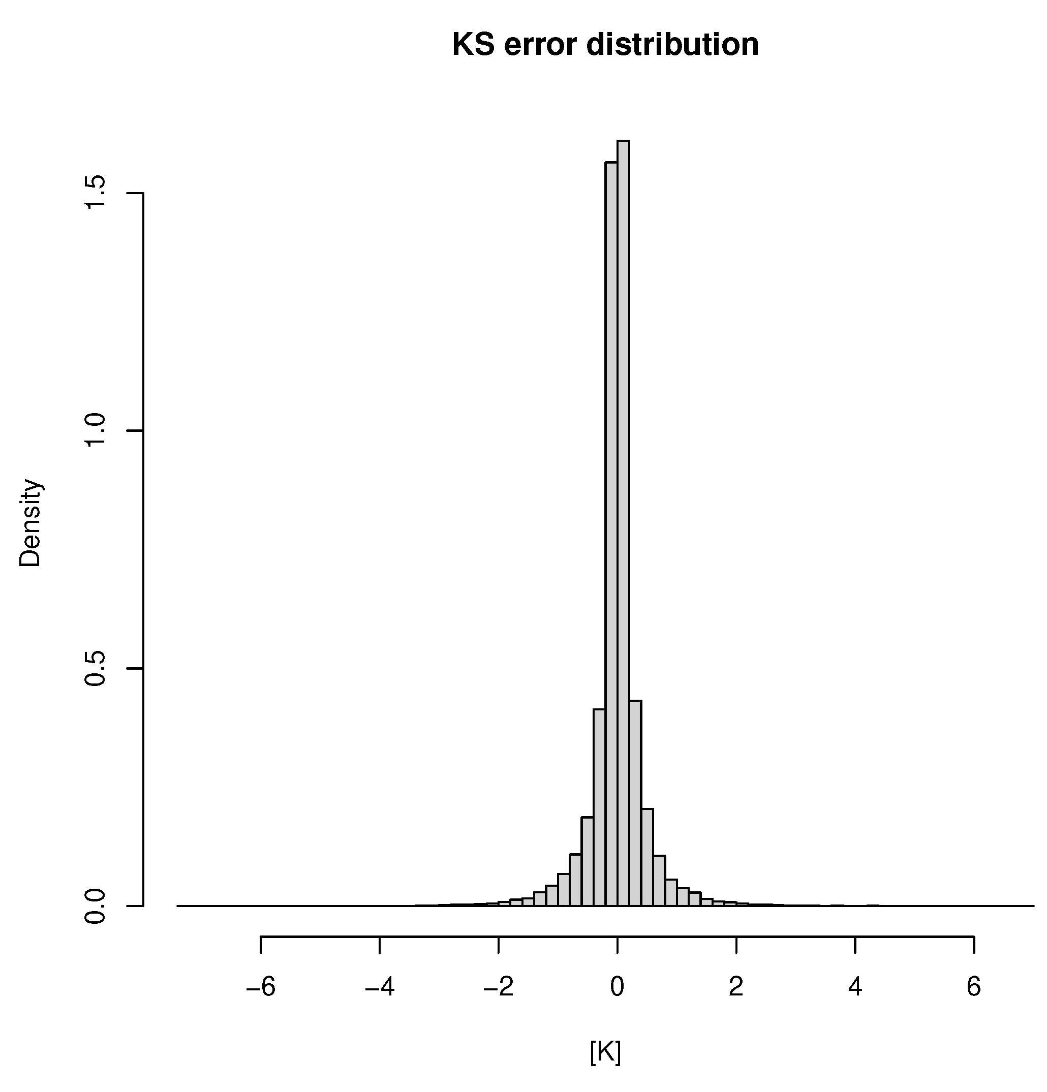
Figure 2. QQ-plots of KS errors at ERA5 levels. Top panel: scaled Student’s t distribution, bottom panel: Normal distribution.

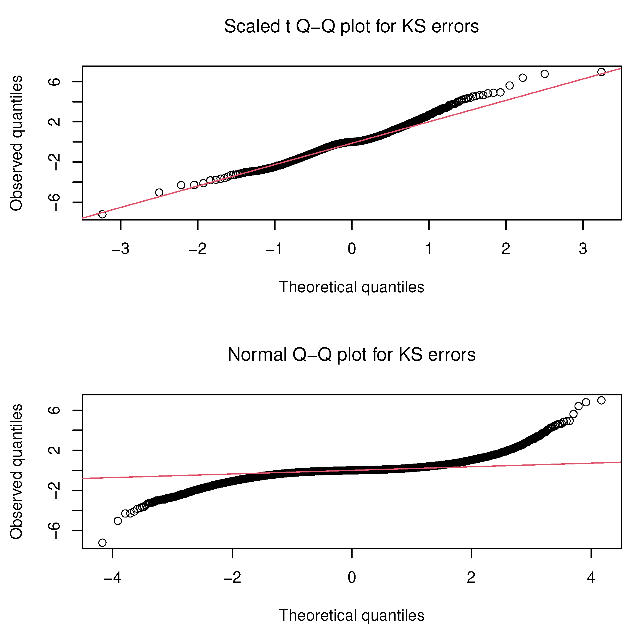
Figure 3. Robust uncertainty profiles. The blue line is the mean absolute error of the KS interpolation; the green line is the mean absolute error of the linear interpolation; the red line is the Median of the KS uncertainty; the black line is the median of GDP measurement uncertainty.

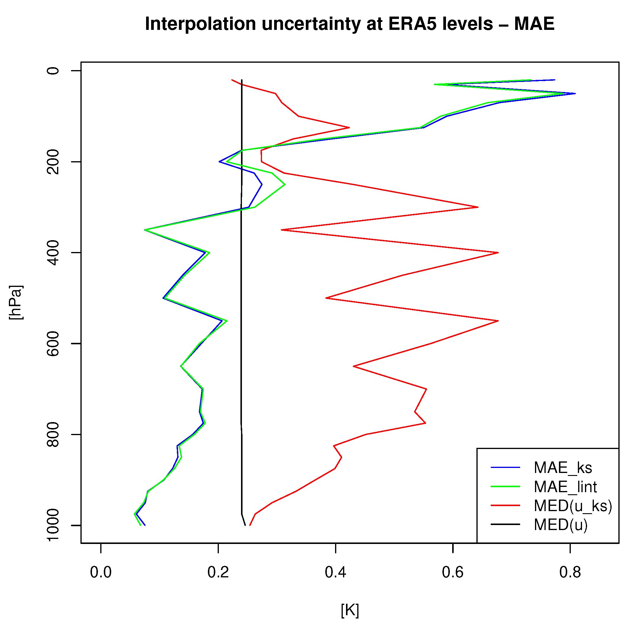
Figure 4. RMSE uncertainty profiles. The blue line is the root mean square error of the KS interpolation; the green line is the mean square error of the linear interpolation; the red line is the quadratic mean of the KS uncertainty; the black line is the quadratic mean of GDP measurement uncertainty.

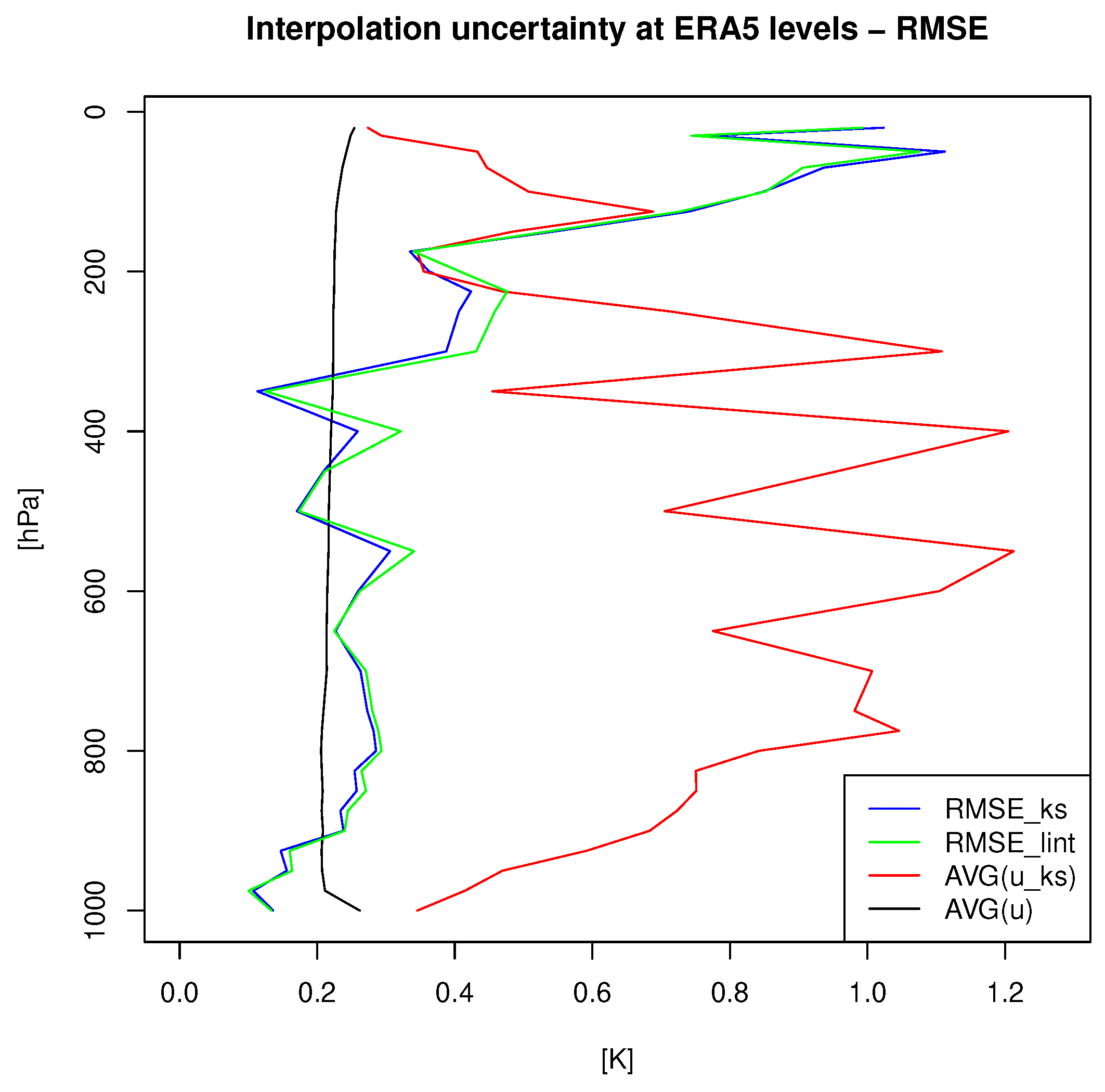
Figure 5. MAE profile by station. Station colours are explained in the panel’s graphic legend. The blue curve is the station average.

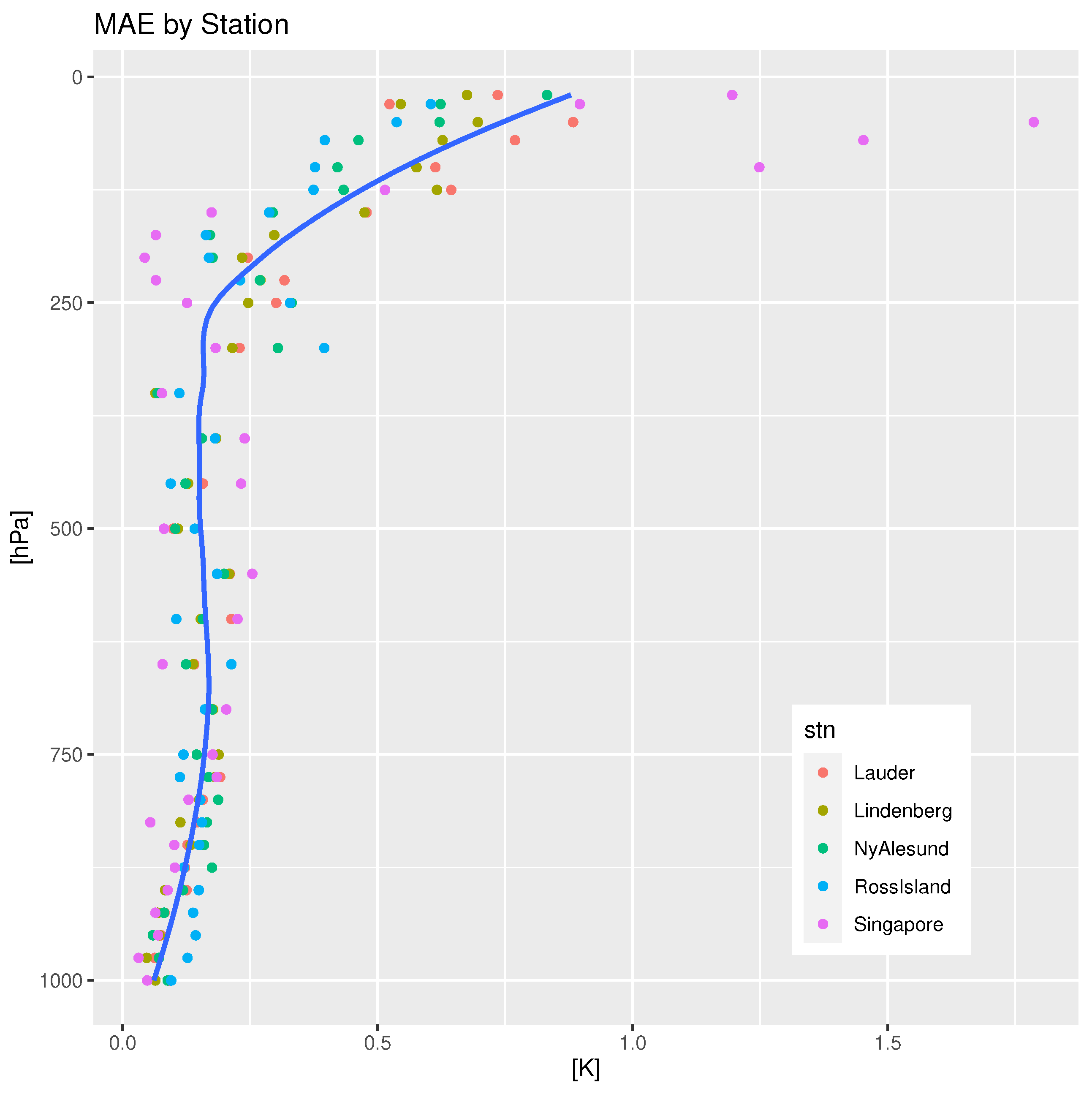
Table 1. GRUAN stations and statistics of data used. RO Obs are used for learning, while ERA5 Obs are used for testing.

Station	Latitude	Longitude	ERA5 Obs	RO Obs	Profiles
Lauder	−45.05 $^{\circ}$	169.68 $^{\circ}$	9 750	14 790	328
Lindenberg	52.21 $^{\circ}$	14.12 $^{\circ}$	11 104	16 564	374
Ny-Alesund	78.92 $^{\circ}$	11.93 $^{\circ}$	6 002	9 040	202
Ross Island	−77.85 $^{\circ}$	166.65 $^{\circ}$	4 378	6 777	174
Singapore	1.30 $^{\circ}$	103.80 $^{\circ}$	2 829	4 100	94
Overall			34 063	51 271	1 172

Table 2. Number of profiles of GRUAN stations by season.

Station	Spring	Summer	Autumn	Winter
Lauder	91	74	84	79
Lindenberg	107	82	91	94
Ny-Alesund	75	36	30	61
Ross Island	57	66	23	28
Singapore	28	19	28	19
Overall	358	277	256	281

Table 3. Number of profiles of GRUAN stations by time of day.

Station	Day	Dusk/dawn	Night
Lauder	163	3	162
Lindenberg	197	49	128
Ny-Alesund	81	54	67
Ross Island	98	40	36
Singapore	32	60	2
Overall	571	206	395

Table 4. k-values of Eq. (6) based on Student’s t distribution for

α = 0.05

and

0.0027

, and tail probabilities for various degrees of freedom

ν

compared to the Gaussian case.

Table 4. k-values of Eq. (6) based on Student’s t distribution for

α = 0.05

and

0.0027

, and tail probabilities for various degrees of freedom

ν

compared to the Gaussian case.

$ν$	$α = 0.05$	$α = 0.0027$	P(\|t\|>3)	P(\|t\|>4)
4	1.96	4.68	1.32E-2	4.80E-3
5	1.99	4.27	1.17E-2	3.59E-3
10	1.99	3.54	7.30E-3	1.19E-3
20	1.98	3.25	4.90E-3	4.00E-4
300	1.96	3.02	2.8E-3	1.00E-4
Gaussian	1.96	3	2.70E-3	1.00E-4

Table 5. KS uncertainty [K] by station. Column details:

M E D (u)

, Median measurement uncertainty;

M E D (u_{K S})

, Median KS interpolation uncertainty;

R M S E_{K S}

, Root mean square interpolation error at ERA5 levels;

M A E_{K S}

, Mean absolute interpolation error;

\hat{σ}

, Maximum t-likelihood scale estimate;

\hat{ν}

, moment estimate of degrees of freedom.

Table 5. KS uncertainty [K] by station. Column details:

M E D (u)

, Median measurement uncertainty;

M E D (u_{K S})

, Median KS interpolation uncertainty;

R M S E_{K S}

, Root mean square interpolation error at ERA5 levels;

M A E_{K S}

, Mean absolute interpolation error;

\hat{σ}

, Maximum t-likelihood scale estimate;

\hat{ν}

, moment estimate of degrees of freedom.

Station	$M E D (u)$	$M E D (u_{K S})$	$R M S E_{K S}$	$M A E_{K S}$	$\hat{σ}$	$\hat{ν}$
Lauder	0.246	0.384	0.498	0.284	0.270	4.392
Lindenberg	0.118	0.374	0.456	0.257	0.243	4.352
Ny-Alesund	0.216	0.379	0.423	0.245	0.235	4.421
Ross Island	0.257	0.268	0.341	0.211	0.209	4.526
Singapore	0.247	0.747	0.702	0.321	0.243	4.334
Overall	0.240	0.369	0.476	0.262	0.242	4.307

Table 6. Standard errors of KS uncertainty [K] by station. Column details: see Table 5.

	Standard errors
Station	$R M S E_{K S}$	$M A E_{K S}$	$\hat{σ}$	$\hat{ν}$
Lauder	0.004	0.004	0.003	0.105
Lindenberg	0.003	0.004	0.002	0.137
Ny-Alesund	0.004	0.004	0.003	0.081
Ross Island	0.004	0.004	0.003	0.102
Singapore	0.009	0.012	0.005	0.044
Overall	0.002	0.002	0.001	0.037

Table 7. KS uncertainty [K] by season. Column details: see Table 5.

Season	Profiles	$M E D (u)$	$M E D (u_{K S})$	$R M S E_{K S}$	$M A E_{K S}$	$\hat{σ}$	$\hat{ν}$
Spring	358	0.24	0.384	0.486	0.262	0.238	4.292
Summer	277	0.247	0.34	0.459	0.251	0.232	4.268
Autumn	256	0.239	0.357	0.479	0.272	0.258	4.494
Winter	281	0.215	0.404	0.477	0.264	0.245	4.267
Overall	1172	0.24	0.369	0.476	0.262	0.242	4.307

Table 8. Standard errors of KS uncertainty [K] by season. Column details: see Table 5.

	Standard errors
Season	Profiles	$R M S E_{K S}$	$M A E_{K S}$	$\hat{σ}$	$\hat{ν}$
Spring	358	0.003	0.004	0.002	0.064
Summer	277	0.004	0.004	0.003	0.102
Autumn	256	0.004	0.005	0.003	0.07
Winter	281	0.004	0.004	0.003	0.062
Overall	1172	0.002	0.002	0.001	0.037

Table 9. KS uncertainty [K] by time of the day for the overall data set and for Lindenberg data. Column details: see Table 5.

Time of day	Profiles	$M E D (u)$	$M E D (u_{K S})$	$R M S E_{K S}$	$M A E_{K S}$	$\hat{σ}$	$\hat{ν}$
Overall
Day	571	0.252	0.342	0.469	0.259	0.241	4.300
Dusk/dawn	206	0.240	0.432	0.510	0.261	0.228	4.277
Night	395	0.239	0.396	0.467	0.266	0.251	4.356
Lindenberg
Day	197	0.153	0.334	0.438	0.254	0.252	4.729
Dusk/dawn	49	0.094	0.409	0.436	0.248	0.241	4.678
Night	128	0.081	0.448	0.490	0.266	0.243	4.221

Table 10. Standard errors of KS uncertainty [K] by season. Column details: see Table 5.

Standard errors
Time of day	Profiles	$R M S E_{K S}$	$M A E_{K S}$	$\hat{σ}$	$\hat{ν}$
Overall
Day	571	0.003	0.003	0.002	0.057
Dusk/dawn	206	0.005	0.006	0.003	0.048
Night	395	0.003	0.004	0.002	0.12
Lindenberg
Day	197	0.004	0.005	0.003	0.071
Dusk/dawn	49	0.008	0.009	0.007	0.091
Night	128	0.006	0.007	0.004	0.127

Table 11. MAE and its standard errors of KS uncertainty [K] by station and time of the day. Column details: see Table 5.

	$M A E_{K S}$			Standard errors
	Day	Dusk/dawn	Night	Day	Dusk/dawn	Night
Lauder	0.283	0.282	0.284	0.006	0.036	0.006
Lindenberg	0.254	0.248	0.266	0.005	0.009	0.007
Ny-Alesund	0.257	0.236	0.239	0.007	0.008	0.007
Ross Island	0.202	0.222	0.223	0.005	0.009	0.009
Singapore	0.333	0.316	0.281	0.021	0.014	0.063

Table 12. RMSE and its standard errors of KS uncertainty [K] by station and time of the day. Column details: see Table 5.

	$R M S E_{K S}$			Standard errors
	Day	Dusk/dawn	Night	Day	Dusk/dawn	Night
Lauder	0.507	0.444	0.489	0.005	0.033	0.005
Lindenberg	0.438	0.436	0.490	0.004	0.008	0.006
Ny-Alesund	0.444	0.411	0.406	0.006	0.007	0.006
Ross Island	0.337	0.353	0.336	0.005	0.008	0.008
Singapore	0.733	0.690	0.557	0.017	0.011	0.051

Disclaimer/Publisher’s Note: The statements, opinions and data contained in all publications are solely those of the individual author(s) and contributor(s) and not of MDPI and/or the editor(s). MDPI and/or the editor(s) disclaim responsibility for any injury to people or property resulting from any ideas, methods, instructions or products referred to in the content.

© 2023 by the authors. Licensee MDPI, Basel, Switzerland. This article is an open access article distributed under the terms and conditions of the Creative Commons Attribution (CC BY) license (http://creativecommons.org/licenses/by/4.0/).

Copyright: This open access article is published under a Creative Commons CC BY 4.0 license, which permit the free download, distribution, and reuse, provided that the author and preprint are cited in any reuse.

Submitted:

06 July 2023

Posted:

07 July 2023

You are already at the latest version

Alerts

Abstract

Keywords:

Subject: Environmental and Earth Sciences - Atmospheric Science and Meteorology

1. Introduction

2. Materials and Methods

2.1. Data

2.2. Interpolation by State Space models

Let

y_{i}

denote the observation of the geophysical quantity of interest, e.g., Temperature [K], at pressure level

p_{i}

i = 1, . . ., n

where n is the number of observations of the profile under consideration. We assume a measurement equation error for

y_{i}

given by

y_{i} = x_{i} + ε_{i} .

(1)

Here,

x_{i}

is the "true" state and

ε_{i}

is the random measurement error with uncertainty

u_{i} = \sqrt{V a r (ε_{i})}

where

V a r ()

is the variance operator. For the state x, we assume locally linear dynamics with respect to pressure, given by

\begin{matrix} x_{i} & = & x_{i - 1} + α_{i} \times (p_{i} - p_{i - 1}) + η_{x, i} \end{matrix}

(2)

\begin{matrix} α_{i} & = & α_{i - 1} + η_{α, i} \end{matrix}

(3)

where

η_{x, i}

and

η_{α, i}

are independent innovation processes with zero mean and variance

σ_{x}^{2}

and

σ_{α}^{2}

respectively. Equation 2 states that apart from the stochastic component

η_{x}

, the geophysical state has a local linear variation with respect to the pressure levels. Equation 3 implies a smooth variation of the coefficient

α

For any pressure level

p^{*} \in [p_{i}, p_{i - 1}]

the optimal estimate of the corresponding state

x^{*}

is given by the following conditional expectation

{\hat{x}}^{*} = E (x^{*} | y_{1}, \dots, y_{n})

(4)

which is readily computed by the Kalman smoother (KS) algorithm under Gaussian assumptions [rif]. In addition, the uncertainty at

p^{*}

is given by

u_{K S} {({\hat{x}}^{*})}^{2} = V a r (x^{*} | y_{1}, \dots, y_{n})

(5)

which also is an output of the above-mentioned KS algorithm.

2.3. Interpolation errors and uncertainty

For each single profile, let us denote by

(y_{i}, p_{i}), i = 1, \dots, n

the observations at GNSS-RO levels, and by

(y_{j}^{*}, p_{j}^{*}), i = 1, \dots, n^{*}

the true values at ERA5 levels. Let

{\hat{y}}_{L I N T, j}

and

{\hat{y}}_{K S, j}

be the linear and Kalman smoother interpolations at ERA5 levels, respectively, and let

e_{L I N T, j}

and

e_{K S, j}

be the corresponding interpolation errors, e.g.

e_{L I N T, j} = {\hat{y}}_{L I N T, j} - y_{j}^{*}

. In the sequel, we focus on altitudes below 10 hPa. As a result, we have

n^{*} = 31

ERA5 levels, and

n \leq 46

GNSS-RO levels, depending on missing data, the average being

n = 44

"Observed" interpolation uncertainty is computed using root mean square error (RMSE) and mean absolute error (MAE). Consider a subset of all profiles, e.g. a station or a season, and denote it by

S

, with profile identifiers

i d \in S

. For methods

m = L I N T, K S

, we have

R M S E_{m, S} = \sqrt{\frac{1}{n^{*} | | S | |} \sum_{j \leq n^{*}, i d \in S} e_{m, i d, j}^{2}}

and

M A E_{m, S} = \sqrt{\frac{1}{n^{*} | | S | |} \sum_{j \leq n^{*}, i d \in S} | | e_{m, i d, j} | |} .

2.4. Non-Gaussian errors

In collocation comparisons, two measurements

m_{1}

and

m_{2}

, with uncertainties

u_{1}

and

u_{2}

, are said to be in agreement [24] if the error

e = m_{1} - m_{2}

, is small, namely

| e | < k \times u_{e}

(6)

for

k = 2

. In this formula,

u_{e}

is the collocation uncertainty. If the uncertainties are uncorrelated and no collocation mismatch affects the measurements, then

u_{e} = \sqrt{u_{1}^{2} + u_{2}^{2}}

. It is well known that

k = 2 (3)

has the interpretation of a statistical test with false rejection probability

α ≅ 5 % (0.27 %)

if e is Gaussian distributed.

If the error distribution has higher tails than the Gaussian distribution, the interpretation of k may be different. Considering a scaled Student’s t distribution, with

ν > 4

degrees of freedom and scale parameter

u_{e} = \sqrt{v a r (e)}

, it is worth noting that the 97.5% percentile is close to the corresponding Gaussian percentile, namely 1.96, for any

ν > 4

. Instead, the probability of large errors, related to

k \geq 3

, for the mentioned t distribution is much larger than the Gaussian counterpart, even if the two measurements come from the same instrument. See some examples in Table 4.

2.5. Inference for the Student’s t distribution

Our case study found that errors have kurtosis, say

k (e)

ν

, and standard error

σ

, depending on the data. This approach allows us to better understand the uncertainty of the data at hand.

In particular, the

ν > 4

parameter is estimated by the method of moments, say

\hat{ν} = 4 + \frac{6}{k (e) - 3}

. Then, the scale

σ

parameter is estimated by the plug-in maximum likelihood method, say

\hat{σ} = {\hat{σ}}_{\hat{ν}}

. Since the sample sizes are large, we do not mind about the loss in efficiency related to the method of moments.

3. Results

\bar{e_{L} - e_{K}} = 0.004 K

, the Spearman correlation coefficient is quite large

r (e_{L}, e_{K}) > 0.95

, and

R M S E (e_{L}, e_{K}) = 0.14 K

. Hence in the sequel, we focus on KS results and omit the subscript K wherever clear.

σ

3.1. Uncertainty by station

It may be noticed from the last column of Table 5 that the tail parameter

\hat{ν}

\hat{σ}

, is quite smaller than RMSE and close to the robust metric given by MAE.

3.2. Uncertainty by altitude

Figure 3 depicts the vertical behaviour of interpolation uncertainty assessed by MAE and compared to the median of measurement uncertainty, u, and KS uncertainty,

u_{K S}

, as in Equation (5). Similarly, Figure 4 describes the RMSE behaviour and compares it to the quadratic means of u and

u_{K S}

It may be noted that both MAE and RMSE interpolation uncertainties are close to the measurement uncertainty below the tropopause, with

M A E < 0.2

K. Instead, around 300 hPa, both show an increase and an even steeper increase above that, with

M A E

The KS interpolation uncertainty (

u_{K S}

) is larger than RMSE and/or MAE below 200 hPa and smaller above. For operational use of

u_{K S}

, we suggest the correction given by Equation (15) of [37].

3.3. Uncertainty by season

ν

and

σ

are quite close for the different seasons. The minimum interpolation uncertainty (either RMSE, MAE or

σ

) is observed in summer with a difference of 0.01−0.02 K with respect to the overall quantity. Again, we have little uncertainty variation among seasons.

3.4. Uncertainty by time of the day

ν

4. Discussion and conclusions

ν = 4.3

degrees of freedom is appropriate. We suggest using MAE and/or

σ

to assess such a non-Gaussian uncertainty. Comparing them to RMSE helps to highlight the high tail impact on uncertainty.

The overall uncertainty of temperature profiles is about 0.25 K for MAE and t-distribution scale parameter

σ

It may be noted that the horizontal and vertical variations dominate the temporal sources of variation considered. Namely, season and time of the day, which can be ignored in this respect.

Author Contributions

Funding

This research received no external funding

Data Availability Statement

Acknowledgments

We wish the express our sincere thanks to GRUAN Lead Center and especially to Michael Sommer for the help and guidance in getting the data and in the release interpretation.

Conflicts of Interest

The authors declare no conflict of interest.

References

Tropea, C.; Yarin, A.L.; Foss, J.F.; others. In Springer handbook of experimental fluid mechanics; Springer, 2007; Vol. 1.
Thompson, O.E.; Eom, J.K.; Wagenhofer, J.R. On the resolution of temperature profile finestructure by the NOAA satellite vertical temperature profile radiometer. Monthly Weather Review 1976, 104, 117–126. [Google Scholar] [CrossRef]
Smith, W.L.; Woolf, H. An intercomparison of meteorological parameters derived from radiosonde and satellite vertical temperature cross sections; Vol. 55, National Environmental Satellite Service, 1974. [Google Scholar]
Shen, W.C.; Smith, W.L.; Woolf, H. An intercomparison of radiosonde and satellite-derived cross sections during the AMTEX; Number 72, National Environmental Satellite Service, 1975. [Google Scholar]
Horn, L.H.; Petersen, R.A.; Whittaker, T.M. Intercomparisons of data derived from Nimbus 5 temperature profiles, rawinsonde observations and initialized LFM model fields. Monthly Weather Review 1976, 104, 1362–1371. [Google Scholar] [CrossRef]
Hilsenrath, E.; Coley, R.; Kirschner, P.; Gammill, B. A rocket ozonesonde for geophysical research and satellite intercomparison. Technical report, 1979.
Trenberth, K.; Jones, P.; Ambenje, P.; Bojariu, R.; Easterling, D.; Klein Tank, A.; Parker, D.; Rahimzadeh, F.; Renwick, J.; Rusticucci, M. others. Chapter 3. Observations: surface and atmospheric climate change. In Climate Change 2007: the physical science basis. Contribution of Working Group I to the fourth assessment report of the Intergovernmental Panel on Climate Change; (Eds S Solomon, D Qin, M Manning, Z Chen, M Marquis, KB Averyt, M Tignor, HL Miller), 2007; pp. 235–336. [Google Scholar]
Foelsche, U.; Scherllin-Pirscher, B.; Ladstädter, F.; Steiner, A.; Kirchengast, G. Refractivity and temperature climate records from multiple radio occultation satellites consistent within 0.05%. Atmospheric Measurement Techniques 2011, 4, 2007–2018. [Google Scholar] [CrossRef]
Anthes, R. Exploring Earth’s atmosphere with radio occultation: contributions to weather, climate and space weather. Atmospheric Measurement Techniques 2011, 4, 1077–1103. [Google Scholar] [CrossRef]
Chen, D.; Rojas, M.; Samset, B.; Cobb, K.; Diongue Niang, A.; Edwards, P.; Emori, S.; Faria, S.; Hawkins, E.; Hope, P.; others. Framing, context, and methods. Climate change 2021, 478, 147–286. [Google Scholar]
Zeng, Z.; Sokolovskiy, S.; Schreiner, W.S.; Hunt, D. Representation of vertical atmospheric structures by radio occultation observations in the upper troposphere and lower stratosphere: Comparison to high-resolution radiosonde profiles. Journal of Atmospheric and Oceanic Technology 2019, 36, 655–670. [Google Scholar] [CrossRef]
Scherllin-Pirscher, B.; Steiner, A.K.; Kirchengast, G.; Schwärz, M.; Leroy, S.S. The power of vertical geolocation of atmospheric profiles from GNSS radio occultation. Journal of Geophysical research: atmospheres 2017, 122, 1595–1616. [Google Scholar] [CrossRef] [PubMed]
Wilhelmsen, H.; Ladstädter, F.; Scherllin-Pirscher, B.; Steiner, A.K. Atmospheric QBO and ENSO indices with high vertical resolution from GNSS radio occultation temperature measurements. Atmospheric Measurement Techniques 2018, 11, 1333–1346. [Google Scholar] [CrossRef]
Stocker, M.; Ladstädter, F.; Wilhelmsen, H.; Steiner, A.K. Quantifying Stratospheric Temperature Signals and Climate Imprints From Post-2000 Volcanic Eruptions. Geophysical Research Letters 2019, 46, 12486–12494. [Google Scholar] [CrossRef] [PubMed]
Chahine, M.T.; Pagano, T.S.; Aumann, H.H.; Atlas, R.; Barnet, C.; Blaisdell, J.; Chen, L.; Divakarla, M.; Fetzer, E.J.; Goldberg, M.; others. AIRS: Improving weather forecasting and providing new data on greenhouse gases. Bulletin of the American Meteorological Society 2006, 87, 911–926. [Google Scholar] [CrossRef]
Hilton, F.; Atkinson, N.; English, S.; Eyre, J. Assimilation of IASI at the Met Office and assessment of its impact through observing system experiments. Quarterly Journal of the Royal Meteorological Society: A journal of the atmospheric sciences, applied meteorology and physical oceanography 2009, 135, 495–505. [Google Scholar] [CrossRef]
Bouillon, M.; Safieddine, S.; Hadji-Lazaro, J.; Whitburn, S.; Clarisse, L.; Doutriaux-Boucher, M.; Coppens, D.; August, T.; Jacquette, E.; Clerbaux, C. Ten-year assessment of IASI radiance and temperature. Remote Sensing 2020, 12, 2393. [Google Scholar] [CrossRef]
Angerer, B.; Ladstädter, F.; Scherllin-Pirscher, B.; Schwärz, M.; Steiner, A.K.; Foelsche, U.; Kirchengast, G. Quality aspects of the Wegener Center multi-satellite GPS radio occultation record OPSv5. 6. Atmospheric Measurement Techniques 2017, 10, 4845–4863. [Google Scholar] [CrossRef]
Gleisner, H.; Lauritsen, K.B.; Nielsen, J.K.; Syndergaard, S. Evaluation of the 15-year ROM SAF monthly mean GPS radio occultation climate data record. Atmospheric Measurement Techniques 2020, 13, 3081–3098. [Google Scholar] [CrossRef]
Steiner, A.K.; Ladstädter, F.; Ao, C.O.; Gleisner, H.; Ho, S.P.; Hunt, D.; Schmidt, T.; Foelsche, U.; Kirchengast, G.; Kuo, Y.H.; others. Consistency and structural uncertainty of multi-mission GPS radio occultation records. Atmospheric Measurement Techniques 2020, 13, 2547–2575. [Google Scholar] [CrossRef]
Blackwell, W.; Milstein, A. A neural network retrieval technique for high-resolution profiling of cloudy atmospheres. IEEE Journal of Selected Topics in Applied Earth Observations and Remote Sensing 2014, 7, 1260–1270. [Google Scholar] [CrossRef]
Susskind, J.; Blaisdell, J.M.; Iredell, L. Improved methodology for surface and atmospheric soundings, error estimates, and quality control procedures: the atmospheric infrared sounder science team version-6 retrieval algorithm. Journal of Applied Remote Sensing 2014, 8, 084994–084994. [Google Scholar] [CrossRef]
Hersbach, H.; Bell, B.; Berrisford, P.; Hirahara, S.; Horányi, A.; Muñoz-Sabater, J.; Nicolas, J.; Peubey, C.; Radu, R.; Schepers, D.; others. The ERA5 global reanalysis. Quarterly Journal of the Royal Meteorological Society 2020, 146, 1999–2049. [Google Scholar] [CrossRef]
Immler, F.; Dykema, J.; Gardiner, T.; Whiteman, D.; Thorne, P.; Vömel, H. Reference quality upper-air measurements: Guidance for developing GRUAN data products. Atmospheric Measurement Techniques 2010, 3, 1217–1231. [Google Scholar] [CrossRef]
Zhongming, Z.; Linong, L.; Xiaona, Y.; Wangqiang, Z.; Wei, L. ; others. Systematic Observation Requirements for Satellite-based Products for Climate Supplemental details to the satellite-based component of the Implementation Plan for the Global Observing System for Climate in Support of the UNFCCC: 2011 update 2011.
Zemp, M.; Chao, Q.; Han Dolman, A.J.; Herold, M.; Krug, T.; Speich, S.; Suda, K.; Thorne, P.; Yu, W. GCOS 2022 Implementation Plan. Global Climate Observing System GCOS.
Rodgers, C.D. Inverse methods for atmospheric sounding: theory and practice. Vol. 2, World scientific, 2000. [Google Scholar]
Weaver, D.; Strong, K.; Schneider, M.; Rowe, P.M.; Sioris, C.; Walker, K.A.; Mariani, Z.; Uttal, T.; McElroy, C.T.; Vömel, H.; others. Intercomparison of atmospheric water vapour measurements at a Canadian High Arctic site. Atmospheric Measurement Techniques 2017, 10, 2851–2880. [Google Scholar] [CrossRef]
Tradowsky, J.S. Radiosonde Temperature Bias Corrections using Radio Occultation Bending Angles as Reference. 2017. Available online: https://rom-saf.eumetsat.int/Publications/reports/romsaf_vs31_rep_v11.pdf (accessed on 20 June 2023).
Gilpin, S.; Rieckh, T.; Anthes, R. Reducing representativeness and sampling errors in radio occultation–radiosonde comparisons. Atmospheric Measurement Techniques 2018, 11, 2567–2582. [Google Scholar] [CrossRef]
Jing, X.; Shao, X.; Liu, T.C.; Zhang, B. Comparison of gruan rs92 and rs41 radiosonde temperature biases. Atmosphere 2021, 12, 857. [Google Scholar] [CrossRef]
Sun, B.; Reale, A.; Seidel, D.J.; Hunt, D.C. Comparing radiosonde and COSMIC atmospheric profile data to quantify differences among radiosonde types and the effects of imperfect collocation on comparison statistics. Journal of Geophysical Research: Atmospheres 2010, 115. [Google Scholar] [CrossRef]
Sun, B.; Reale, T.; Schroeder, S.; Pettey, M.; Smith, R. On the accuracy of Vaisala RS41 versus RS92 upper-air temperature observations. Journal of Atmospheric and Oceanic Technology 2019, 36, 635–653. [Google Scholar] [CrossRef]
Sun, B.; Calbet, X.; Reale, A.; Schroeder, S.; Bali, M.; Smith, R.; Pettey, M. Accuracy of Vaisala RS41 and RS92 upper tropospheric humidity compared to satellite hyperspectral infrared measurements. Remote Sensing 2021, 13, 173. [Google Scholar] [CrossRef]
Ho, S.p.; Peng, L.; Vömel, H. Characterization of the long-term radiosonde temperature biases in the upper troposphere and lower stratosphere using COSMIC and Metop-A/GRAS data from 2006 to 2014. Atmospheric Chemistry and Physics 2017, 17, 4493–4511. [Google Scholar] [CrossRef]
ROMSAF. Product Archive. 2017. Available online: https://rom-saf.eumetsat.int/product_archive.php (accessed on 19 June 2023).
Fassò, A.; Sommer, M.; von Rohden, C. Interpolation uncertainty of atmospheric temperature profiles. Atmospheric Measurement Techniques 2020, 13, 6445–6458. [Google Scholar] [CrossRef]
Colombo, P.; Fassò, A. Quantifying the interpolation uncertainty of radiosonde humidity profiles. Measurement Science and Technology 2022, 33, 074001. [Google Scholar] [CrossRef]
Virman, M.; Bister, M.; Räisänen, J.; Sinclair, V.A.; Järvinen, H. Radiosonde comparison of ERA5 and ERA-Interim reanalysis datasets over tropical oceans. Tellus A: Dynamic Meteorology and Oceanography 2021, 73, 1–7. [Google Scholar] [CrossRef]
Hoffmann, L.; Spang, R. An assessment of tropopause characteristics of the ERA5 and ERA-Interim meteorological reanalyses. Atmospheric Chemistry and Physics 2022, 22, 4019–4046. [Google Scholar] [CrossRef]
Imfeld, N.; Haimberger, L.; Sterin, A.; Brugnara, Y.; Brönnimann, S. Intercomparisons, error assessments, and technical information on historical upper-air measurements. Earth System Science Data 2021, 13, 2471–2485. [Google Scholar] [CrossRef]
Nash, J.; Oakley, T.; Vömel, H.; Wei, L. WMO Intercomparison of High Quality Radiosonde Systems (12 July–3 August 2010; Yangjiang, China), WMO/TD-No. 1580; IOM Report-No. 107, 2011.
Navas-Guzmán, F.; Kämpfer, N.; Schranz, F.; Steinbrecht, W.; Haefele, A. Intercomparison of stratospheric temperature profiles from a ground-based microwave radiometer with other techniques. Atmospheric chemistry and physics 2017, 17, 14085–14104. [Google Scholar] [CrossRef]
Dirksen, R.J.; Sommer, M.; Immler, F.J.; Hurst, D.F.; Kivi, R.; Vömel, H. Reference quality upper-air measurements: GRUAN data processing for the Vaisala RS92 radiosonde. Atmospheric Measurement Techniques 2014, 7, 4463–4490. [Google Scholar] [CrossRef]
Robert H. Shumway, D.S.S. In Time Series Analysis and Its Applications With R Examples; Vol. 1, Springer, 2017.
M. Sommer, C. M. Sommer, C. von Rohden, T.S.P.O.T.N.G.R.H.J.P.S.R.D. GRUAN characterisation and data processing of the Vaisala RS41 radiosonde. GRUAN Technical Document 8, 2023.
Survo, P., e. a. Atmospheric Temperature and Humidity Measurements of Vaisala Radiosonde RS41, in WMO Technical Conference on Meteorological and Environmental Instruments and Methods of Observations. Saint Petersburg, Russian Federation, 07-09 July 2014, P3(16), IOM Report, 116, WMO, 2014.
HUANG, Y., e. a. A novel robust Gaussian–Student’s t mixture distribution based Kalman filter. IEEE Transactions on signal Processing 2019, 67, 3606–3620. [Google Scholar] [CrossRef]

Figure 1. Frequency distribution of KS errors at ERA5 levels.

Figure 2. QQ-plots of KS errors at ERA5 levels. Top panel: scaled Student’s t distribution, bottom panel: Normal distribution.

Figure 5. MAE profile by station. Station colours are explained in the panel’s graphic legend. The blue curve is the station average.

Table 1. GRUAN stations and statistics of data used. RO Obs are used for learning, while ERA5 Obs are used for testing.

Station	Latitude	Longitude	ERA5 Obs	RO Obs	Profiles
Lauder	−45.05 $^{\circ}$	169.68 $^{\circ}$	9 750	14 790	328
Lindenberg	52.21 $^{\circ}$	14.12 $^{\circ}$	11 104	16 564	374
Ny-Alesund	78.92 $^{\circ}$	11.93 $^{\circ}$	6 002	9 040	202
Ross Island	−77.85 $^{\circ}$	166.65 $^{\circ}$	4 378	6 777	174
Singapore	1.30 $^{\circ}$	103.80 $^{\circ}$	2 829	4 100	94
Overall			34 063	51 271	1 172

Table 2. Number of profiles of GRUAN stations by season.

Station	Spring	Summer	Autumn	Winter
Lauder	91	74	84	79
Lindenberg	107	82	91	94
Ny-Alesund	75	36	30	61
Ross Island	57	66	23	28
Singapore	28	19	28	19
Overall	358	277	256	281

Table 3. Number of profiles of GRUAN stations by time of day.

Station	Day	Dusk/dawn	Night
Lauder	163	3	162
Lindenberg	197	49	128
Ny-Alesund	81	54	67
Ross Island	98	40	36
Singapore	32	60	2
Overall	571	206	395

Table 4. k-values of Eq. (6) based on Student’s t distribution for

α = 0.05

and

0.0027

, and tail probabilities for various degrees of freedom

ν

compared to the Gaussian case.

Table 4. k-values of Eq. (6) based on Student’s t distribution for

α = 0.05

and

0.0027

, and tail probabilities for various degrees of freedom

ν

compared to the Gaussian case.

$ν$	$α = 0.05$	$α = 0.0027$	P(\|t\|>3)	P(\|t\|>4)
4	1.96	4.68	1.32E-2	4.80E-3
5	1.99	4.27	1.17E-2	3.59E-3
10	1.99	3.54	7.30E-3	1.19E-3
20	1.98	3.25	4.90E-3	4.00E-4
300	1.96	3.02	2.8E-3	1.00E-4
Gaussian	1.96	3	2.70E-3	1.00E-4

Table 5. KS uncertainty [K] by station. Column details:

M E D (u)

, Median measurement uncertainty;

M E D (u_{K S})

, Median KS interpolation uncertainty;

R M S E_{K S}

, Root mean square interpolation error at ERA5 levels;

M A E_{K S}

, Mean absolute interpolation error;

\hat{σ}

, Maximum t-likelihood scale estimate;

\hat{ν}

, moment estimate of degrees of freedom.

Table 5. KS uncertainty [K] by station. Column details:

M E D (u)

, Median measurement uncertainty;

M E D (u_{K S})

, Median KS interpolation uncertainty;

R M S E_{K S}

, Root mean square interpolation error at ERA5 levels;

M A E_{K S}

, Mean absolute interpolation error;

\hat{σ}

, Maximum t-likelihood scale estimate;

\hat{ν}

, moment estimate of degrees of freedom.

Station	$M E D (u)$	$M E D (u_{K S})$	$R M S E_{K S}$	$M A E_{K S}$	$\hat{σ}$	$\hat{ν}$
Lauder	0.246	0.384	0.498	0.284	0.270	4.392
Lindenberg	0.118	0.374	0.456	0.257	0.243	4.352
Ny-Alesund	0.216	0.379	0.423	0.245	0.235	4.421
Ross Island	0.257	0.268	0.341	0.211	0.209	4.526
Singapore	0.247	0.747	0.702	0.321	0.243	4.334
Overall	0.240	0.369	0.476	0.262	0.242	4.307

Table 6. Standard errors of KS uncertainty [K] by station. Column details: see Table 5.

	Standard errors
Station	$R M S E_{K S}$	$M A E_{K S}$	$\hat{σ}$	$\hat{ν}$
Lauder	0.004	0.004	0.003	0.105
Lindenberg	0.003	0.004	0.002	0.137
Ny-Alesund	0.004	0.004	0.003	0.081
Ross Island	0.004	0.004	0.003	0.102
Singapore	0.009	0.012	0.005	0.044
Overall	0.002	0.002	0.001	0.037

Table 7. KS uncertainty [K] by season. Column details: see Table 5.

Season	Profiles	$M E D (u)$	$M E D (u_{K S})$	$R M S E_{K S}$	$M A E_{K S}$	$\hat{σ}$	$\hat{ν}$
Spring	358	0.24	0.384	0.486	0.262	0.238	4.292
Summer	277	0.247	0.34	0.459	0.251	0.232	4.268
Autumn	256	0.239	0.357	0.479	0.272	0.258	4.494
Winter	281	0.215	0.404	0.477	0.264	0.245	4.267
Overall	1172	0.24	0.369	0.476	0.262	0.242	4.307

Table 8. Standard errors of KS uncertainty [K] by season. Column details: see Table 5.

	Standard errors
Season	Profiles	$R M S E_{K S}$	$M A E_{K S}$	$\hat{σ}$	$\hat{ν}$
Spring	358	0.003	0.004	0.002	0.064
Summer	277	0.004	0.004	0.003	0.102
Autumn	256	0.004	0.005	0.003	0.07
Winter	281	0.004	0.004	0.003	0.062
Overall	1172	0.002	0.002	0.001	0.037

Table 9. KS uncertainty [K] by time of the day for the overall data set and for Lindenberg data. Column details: see Table 5.

Time of day	Profiles	$M E D (u)$	$M E D (u_{K S})$	$R M S E_{K S}$	$M A E_{K S}$	$\hat{σ}$	$\hat{ν}$
Overall
Day	571	0.252	0.342	0.469	0.259	0.241	4.300
Dusk/dawn	206	0.240	0.432	0.510	0.261	0.228	4.277
Night	395	0.239	0.396	0.467	0.266	0.251	4.356
Lindenberg
Day	197	0.153	0.334	0.438	0.254	0.252	4.729
Dusk/dawn	49	0.094	0.409	0.436	0.248	0.241	4.678
Night	128	0.081	0.448	0.490	0.266	0.243	4.221

Table 10. Standard errors of KS uncertainty [K] by season. Column details: see Table 5.

Standard errors
Time of day	Profiles	$R M S E_{K S}$	$M A E_{K S}$	$\hat{σ}$	$\hat{ν}$
Overall
Day	571	0.003	0.003	0.002	0.057
Dusk/dawn	206	0.005	0.006	0.003	0.048
Night	395	0.003	0.004	0.002	0.12
Lindenberg
Day	197	0.004	0.005	0.003	0.071
Dusk/dawn	49	0.008	0.009	0.007	0.091
Night	128	0.006	0.007	0.004	0.127

Table 11. MAE and its standard errors of KS uncertainty [K] by station and time of the day. Column details: see Table 5.

	$M A E_{K S}$			Standard errors
	Day	Dusk/dawn	Night	Day	Dusk/dawn	Night
Lauder	0.283	0.282	0.284	0.006	0.036	0.006
Lindenberg	0.254	0.248	0.266	0.005	0.009	0.007
Ny-Alesund	0.257	0.236	0.239	0.007	0.008	0.007
Ross Island	0.202	0.222	0.223	0.005	0.009	0.009
Singapore	0.333	0.316	0.281	0.021	0.014	0.063

Table 12. RMSE and its standard errors of KS uncertainty [K] by station and time of the day. Column details: see Table 5.

	$R M S E_{K S}$			Standard errors
	Day	Dusk/dawn	Night	Day	Dusk/dawn	Night
Lauder	0.507	0.444	0.489	0.005	0.033	0.005
Lindenberg	0.438	0.436	0.490	0.004	0.008	0.006
Ny-Alesund	0.444	0.411	0.406	0.006	0.007	0.006
Ross Island	0.337	0.353	0.336	0.005	0.008	0.008
Singapore	0.733	0.690	0.557	0.017	0.011	0.051

MDPI Initiatives

Important Links

Choose an area of interest and we will send you notifications of new preprints at your preferred frequency.

Disclaimer

On the Interpolation Error Distribution in Collocation Comparison of Atmospheric Profiles

Abstract

1. Introduction

2. Materials and Methods

2.1. Data

2.2. Interpolation by State Space models

2.3. Interpolation errors and uncertainty

2.4. Non-Gaussian errors

2.5. Inference for the Student’s t distribution

3. Results

3.1. Uncertainty by station

3.2. Uncertainty by altitude

3.3. Uncertainty by season

3.4. Uncertainty by time of the day

4. Discussion and conclusions

Author Contributions

Funding

Data Availability Statement

Acknowledgments

Conflicts of Interest

References

Abstract

1. Introduction

2. Materials and Methods

2.1. Data

2.2. Interpolation by State Space models

2.3. Interpolation errors and uncertainty

2.4. Non-Gaussian errors

2.5. Inference for the Student’s t distribution

3. Results

3.1. Uncertainty by station

3.2. Uncertainty by altitude

3.3. Uncertainty by season

3.4. Uncertainty by time of the day

4. Discussion and conclusions

Author Contributions

Funding

Data Availability Statement

Acknowledgments

Conflicts of Interest

References

MDPI Initiatives

Important Links

Subscribe