Preprint
Article

CFD Model Verification and Aerodynamic Analysis in Large-Scaled Venlo Greenhouse Complex for Tomato Cultivation

Altmetrics

Downloads

196

Views

55

Comments

0

A peer-reviewed article of this preprint also exists.

Submitted:

12 July 2023

Posted:

13 July 2023

You are already at the latest version

Alerts
Abstract
To address the challenges of climate change and food security, the establishment of smart farm complexes is necessary. While there have been numerous studies on the productivity and environmental control of individual greenhouses, research on greenhouse complexes is considerably limited. Conducting environmental studies during the design phase of these complexes poses financial constraints and practical limitations in terms of on-site experiments. To identify potential issues that may arise when developing large-scale greenhouse complexes, it is possible to utilize modeling techniques using Computational Fluid Dynamics (CFD) to assess environmental concerns and location issues before constructing the facilities. Consequently, simulating large-scale CFD models that incorporate multiple greenhouses and atmospheric conditions simultaneously presents significant numerical challenges. The objective of this study was to develop a guideline for verifying CFD models for a large-scale Venlo greenhouse, where acquiring field data before construction is not feasible for designing a greenhouse complex. The verification processes of the CFD models were conducted using 2D and 3D iterative simulations of a 2-hectare greenhouse model, using the improved Grid Independence Test (GIT) and wall Y+ approaches. Subsequently, the aerodynamic characteristics were analyzed in a 3D greenhouse model to access its performance when the wind direction was 90° in summer season. The findings revealed that a grid resolution of 0.8 meters and a first layer height of 0.04 meters were suitable for developing large-scale greenhouse models, resulting in a low Root Mean Square Error (RMSE) of 3.9% and a high coefficient of determination (R2) of 0.968. This process led to a significant reduction of 38% in the number of grid cells. These results will serve as design standards for large-scale greenhouses.
Keywords: 
Subject: Engineering  -   Other

1. Introduction

The recent issue of climate change has led to an increase in the annual global-average air temperature and unpredictable precipitation patterns [1]. As a result, open field cultivation has become cost inefficient, unreliable, and has contributed to an inconsistent food production system [2,3]. The rise in population has further exacerbated food insecurity challenges in numerous countries worldwide [4]. To tackle these challenges, greenhouse cultivation has emerged as an effective solution [5]. Under the unfavorable climate conditions, it is necessary to establish large scale protected agricultural facilities to meet the increasing population pressure on food production systems. Consequently, the Korean government recently initiated a campaign to develop large-scale greenhouse complexes on reclaimed land aimed at fostering seasonal independent-production and export of high-quality horticultural products [6]
To develop large-scale greenhouse systems for commercial purposes, it is crucial to identify and understand environmental factors. Current greenhouse designs aim to optimize plant growth parameters such as temperature, humidity, light, and carbon dioxide levels, while also considering energy efficiency [7,8]. Heating and cooling in greenhouses contribute to 50 to 80% of the total energy demand and associated costs [9]. The distribution of temperature, humidity, carbon dioxide, and energy efficiency is significantly influenced by the ventilation characteristics of the structure [10]. In naturally ventilated greenhouses, ventilation efficiency is greatly influenced by factors such as greenhouse structural design, prevailing weather conditions, crop type, and greenhouse orientation [11]. As a result, many studies have been conducted to evaluate the effectiveness of natural ventilation on the internal micro-environment of greenhouses [12,13,14,15,16,17,18,19]. These studies have utilized both field experiments and Computation Fluid Dynamics (CFD) modeling and simulations to investigate greenhouse microenvironment and structural safety in relation to environmental problems [20,21,22,23]. Additionally, research has been conducted on greenhouses built on Korean reclaimed lands [24].
Modeling and simulating large greenhouse system offer an alternative approach to address challenges associated with field experiments [25]. However, validating these large-scale models poses difficulties due to the unavailability of field data from such structures before construction. Moreover, in order to achieve acceptable model accuracy, the computational grid must be sufficiently fine to minimize computational errors [26]. Consequently, modeling large-scale structures with a fine computational grid results in a large volume of computational grid cells, presenting significant limitations in computational capability and time. A similar issue was also highlighted in a study by [27], they encountered similar challenges when dealing with a CFD-DEM coupled model of large-scale gas-liquid-solid three-phase flows. To overcome the scale complexity, they employed a flow particle scale-up approach. [28] developed a CFD model to assess wind-driven natural ventilation in single-span greenhouses built on reclaimed coastal land, utilizing 20 years of weather data from 72 weather stations. They validated the model using particle image velocimetry (PIV) and wind tunnel results. [29] provides detailed procedures and guidelines for applying CFD in modeling the indoor environment of structures. These guidelines cover aspects such as modeling, discretization, verification, validation processes, data acquisition, selection of simulation regime, turbulence models, and reporting of CFD results. However, previous models have mainly focused on small-scale greenhouses of less than 1 hectare, making them less suitable for developing design and control strategies for large-scale greenhouses and greenhouse complexes considering the internal microenvironment of greenhouses. And procedural guidelines are not enough for specifically addressing the design and validation of large-scale CFD models for agricultural structures, where the scale is a limiting factor for both modeling and data acquisition processes.
The main objective of this study was to propose a large-scale greenhouse CFD model and establish an accuracy verification procedure using grid independence test and wall boundary conditions. By utilizing the verified CFD model, a three-dimensional, 2-hectare Venlo greenhouse was designed and simulated to investigate crucial factors such as internal environmental distributions and ventilation efficiency based on airflow patterns corresponding to external environment.

2. Materials and Methods

2.1. Computational fluid dynamics

The computational fluid dynamics (CFD) method enables the explicit calculation of airflow patterns through the numerical solution of the Reynolds-averaged form of the Navier-Stokes equations [18,30]. In the case of a steady-state, three-dimensional flow, the classical equations governing mass, momentum, energy, and concentration are expressed as follows:
t + x j u j = x j Γ ϕ x j + s ,
where is the variable of interest, the three velocity components u j m s 1 , the temperature T (K), and the specific humidity Γ ϕ and S ϕ represent the diffusion coefficient and source term of . The details of the equations were describe in [31]. [24] conducted a study to determine the most suitable turbulence model for greenhouse CFD modelling purposes. They reported Renormalization-group (RNG) k-epsilon turbulent model to yield the highest level of accuracy, with an R2 value of 0.99. In this study, the RNG k-epsilon model, in conjunction with enhanced wall functions was selected. The RNG k-epsilon model can be numerically expressed using Equation 2 and 3.
ρ d κ d t = x i α k μ e f f . k x i + G k + G b ρ ε Y M ,
In addition to the turbulence model mentioned earlier, the Boussinesq model was employed to account for the effect of gravity. This was achieved by including the buoyancy force resulting from air density variations as a source term in the momentum equation [32]. The simulation software used for this study was Ansys Fluent, version 2022 R2, which utilizes a pressure-based finite-volume discretization code (Ansys Inc., USA).

2.2. Target greenhouse type, crop and location
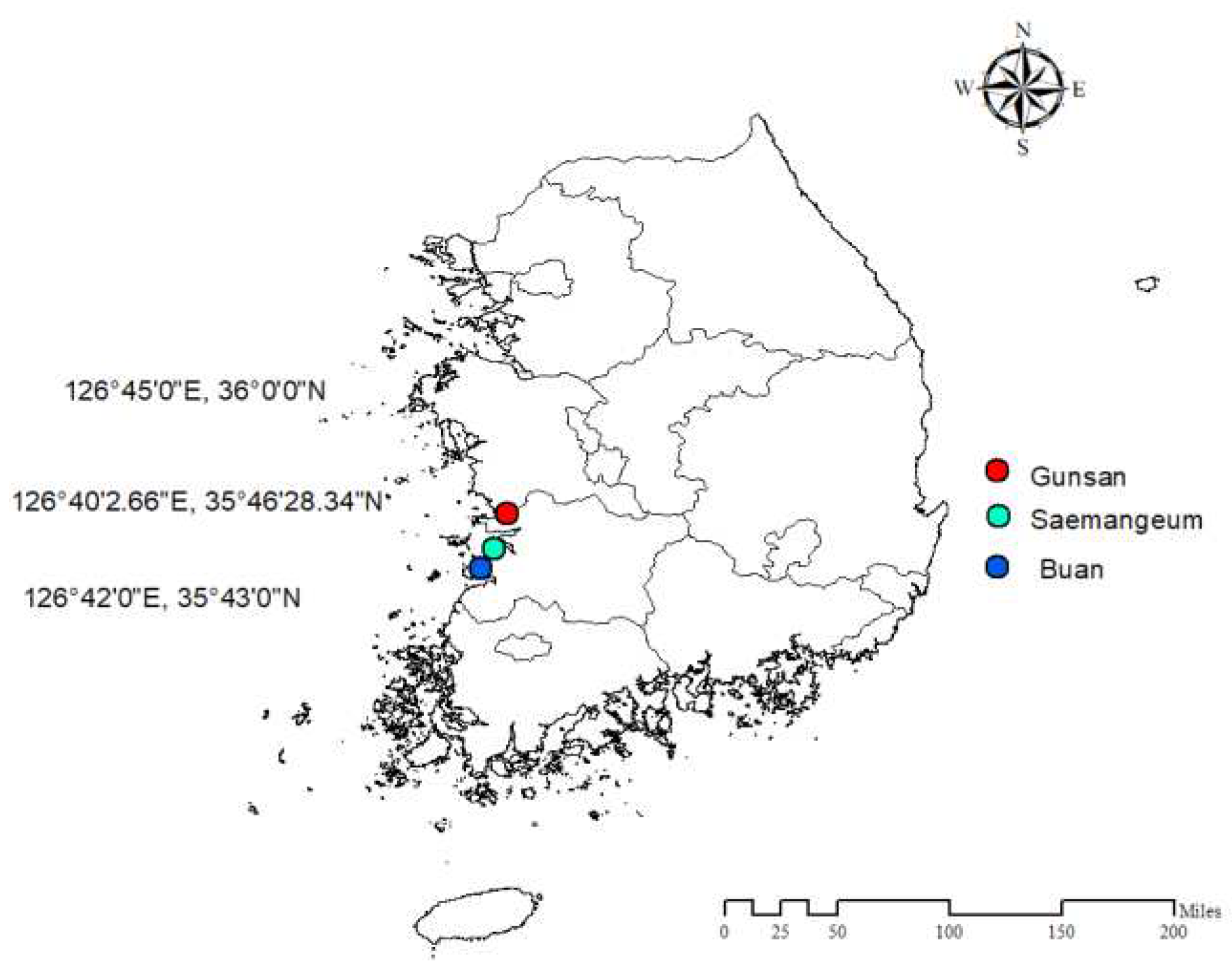
The target area for this study was Saemangeum reclaimed land (35°46'28.34"N, 126°40'2.66"E) located between Gunsan (E 1260 45',N360 00) and Buan ( 126042, N35043) in Korea. The weather conditions of the target area used in this study were average weather conditions for Buan and Gunsan.
Figure 1. Target reclaimed land location and weather stations used for data analysis.
Preprints 79290 g001
In Korea, greenhouse cultivation is dominated by among other crops; Paprika, Green pepper, straw berry and Tomatoes. Considering major crop growth factors and crop characteristics like water consumption, optimal micro-environmental requirement, ventilation requirement and height, tomato crop has average values compared to the other major crops. therefore to design a greenhouse system that is applicable to a wide range of crops, tomato was considered as target crop for this study.
The target greenhouse type was Venlo because of its popularity in the current smart farm system in Korea. studies report that multi-span Venlo greenhouse account 80% of greenhouse types adopted for smart farming in Korea. Also Venlo greenhouses have a relatively larger Eave height of about 6m which can accommodate a large range of crop heights.

2.3. Crop canopy design

The presence of crops in greenhouses has a great impact on natural ventilation efficiency and distribution of micro-environment. The effect of crop canopy was modeled by considering the crop domain as porous media with momentum loss effect. The Darcy Forchheimer equation was used to introduce the drag force induced by crops canopy into the CFD model as a source term, shown in Equation 4. [22,30,33,34].
S = μ κ p u + C F K P ρ u 2 ,
S = I L A v ρ C D u 2 = C F K P ρ u 2 ,
S = I L A v C D u 2 ,
c 2 = 2 C F K p 0.5 ,
where ρ k g m 3   is the fluid density, μ k g s 1 m 1 is the dynamic viscosity, k p m 2 is the permeability of the porous media and C F is the non-linear momentum loss-term. For flow characteristics through plant canopy, only the nonlinear quadratic term of Equation 4 is considered. The momentum source term can also be expressed in terms of unit volume of the canopy as in Equation 5. Equating Equations 4 and 5 and considering only the non-linear momentum loss term, the momentum source term reduces to as in Equation 6. The porous media characteristics of the crop canopy were described by the inertial resistance factor ( c 2 ) given by Equation 7 [35]

2.4. Atmospheric boundary layer (ABL) design

The impact of the external environment on the internal micro-environment of the greenhouse was considered by designing the wind characteristics in the immediate vicinity of the greenhouse. The size of the computational domain representing the external environment was determined based on recommendations from [34,36,37]. For both 2D and 3D models, the overall height of the computational domain was set to 10 times the height (H) of the model greenhouse, while the horizontal extent was set to 15 times. [24] determined the aerodynamic surface characteristics of reclaimed land in Korea. These findings, combined with 11-year average weather data for summer, were used to develop wind and turbulence profiles using the log law method (Equation 8) described by [38], and the specific equations involved in this method are represented by Equations 8, 9, and 10.
U z = u k ln z + z 0 z 0 ,
k z = u 2 C μ . ,
ε z = u 3 k z + z 0 ,
where U(z) ( m s 1 ) is the vertical wind speed, z (m) is the reference height, u is the shear velocity ( m s 1 ) , k is the Karman constant, z 0 is roughness height (m) and C μ is the empirical constant. The turbulent kinetic energy ε z m 2 s 3 , wind profile and turbulent kinetic energy dissipation rate(k) for reclaimed lands were designed using surface roughness factor. The designed profiles were applied as inlet boundary conditions to the model using compiled User Defined Functions (UDFs) in the main CFD code; Ansys fluent software. The parameters and values used in the design are summarized in Table 1.

2.5. Model verification theories

2.5.1. GIT

The GIT is a crucial step in validating CFD simulations. It involves systematic refinement of the numerical grid used to discretize the fluid domain and comparing the resulting solution with a reference solution or experimental data. The goal is to determine the minimum grid resolution required to obtain a converged and accurate solution. This is to ensure that the numerical solution is accurate and reliable, while minimizing computational costs [29,39]. The need for a grid independence test arises from the fact that the numerical solution of the governing equations of fluid flow is based on discretizing the domain into a finite set of grid points. The accuracy of the solution depends on the resolution of the grid. A coarse grid may lead to numerical errors and inaccuracies in the solution, while a fine grid may result in excessive computational costs and unnecessary detail [40]. Several methods have been used to perform grid independence test: Richardson extrapolation method, Grid convergence index (GCI), and the grid refinement study are the commonest methods.

2.5.2. Wall Y+

In turbulence models, viscous fluid-flow at larger Reynolds numbers, the fluid's inertia overcomes the viscous stresses, and the flow becomes unsteady, termed as turbulent flow. All flows of practical engineering interest are virtually turbulent [41]. Several studies have also reported flow inside greenhouses to be typically turbulent. The turbulent flow velocity profile near the wall has three distinct layers: the viscous sub layer, the log layer, and the defect layer. The log layer is the portion of the boundary layer where the sub layer and defect layer merge and the law of the wall accurately represents the velocity. Turbulence vanishes near the walls due to the no-slip boundary condition for the velocity as well as the blocking effect caused by the wall. In the viscous sub layer, an adequate numerical resolution of a solution is required which calls for a very fine mesh. This is because of the thinness of the sub layer and high solution gradients. This makes calculations time consuming and may be impractical for large scale industrial application [42]. Fine numerical mesh and wall functions approaches are commonly employed in CFD calculation of turbulent flow near walls to resolve the thin near-wall sub-layer. The wall functions approach requires less computational effort and is thus strongly favored by industrial calculations. However, their performance is often poor because of inappropriate implementation and partly because the schemes themselves have inherent limitations [43].
Wall Y+ is a dimensionless number that determines the flow region where the turbulence model resolves the boundary layer. It depends on the height of the first layer cell from the wall boundaries. Each turbulence model operates in a specific range of Y+ to accurately resolve the boundary layer. For RNG model, wall Y+ value should range between 30 to 300 [44]. This range was imperatively used to determine the corresponding first layer height (YP) for the model using methods in Equation 11.
Y + = u τ a i r Y P V a i r ;   u τ a i r = τ w a l l ρ , R e = ρ U L V a i r ,   C f = 0.026 R e 1 7 ,   τ w a l l = c f ρ U 2 2 ,
where Re is Reynolds number, ρ is air density k g · m 3 , L is the reference length(m), C f is an empirical constant, U is the free stream velocity of air ( m · s 1 ), τ w a l l is the wall shear force ( k g m 1 · s 2 ).
In the current study, the grid refinement approach was used to perform the grid independent study for establishing the most optimal grid conditions (see Section 2.5.1). Wall functions and Y+ approaches were used to optimize model accuracy. For verification, Statistical indices R2 and RMSE were used as judgment criteria for grid optimal conditions efficient for designing large scale greenhouse models. The grid condition that satisfies the 5% requirement or lower for RMSE and the value of 0.95 or higher for R2 were defined as the optimal conditions for model verification.

2.6. Ventilation efficiency theories.

To evaluate the natural ventilation, the tracer gas decay method (TGD) was used considering CO2 gas. TGD is a qualitative method that uses a tracer gas introduced in the structure to estimate the ventilation rates. It is based on the analysis of decay rate of the tracer gas inside the study structure. TGD considers the greenhouse internal air flow characteristics, ventilator configuration and the external environment therefore, it has been widely used to calculate local ventilation rates inside structures. For this study, TGD approach was used to estimate the local ventilation rates for the model 2 ha greenhouse. The air exchange rates were calculated using Equation.
A E T G D = ln C 0 C t t t 0
where C0 is the concentration of the tracer gas (ppm) when time is 0 sec. Ct is the concentration of at time t (sec), AETGD is air exchange rate (AER.min-1).
Ventilation requirement was used to evaluate the performance of natural ventilation of the greenhouse. Ventilation requirement of a structure can be described as the amount of ventilation rate required to maintain optimal environment such as temperature, relative humidity, CO2 etc. inside the structure for proper crop growth. In this study, ventilation requirement for temperature control method (Korea Rural Community Corporation., 1997) approach was used to estimate the ventilation requirement (Equation 8). The parameters used for the evaluation are shown in Table 2.
V R = 1 C V α τ S 1 f A f T k A c 1 V

2.7. Study procedure

The overall simulation process was conducted in 3 main stages: weather analysis, greenhouse CFD model design and verification as shown in Figure 2.

2.7.1. Weather analysis

20 years weather data for target reclaimed was analyzed, and average summer data was used to design the CFD model boundary conditions, vertical wind profile and turbulence intensity. The most frequent wind speed range at both the weather stations was 0.5-3.3 m·s-1. The annual summer wind speed was then determined as 3.08 m·s-1 and was used as the speed at the reference height velocity.

2.7.2. Greenhouse CFD model design and simulation
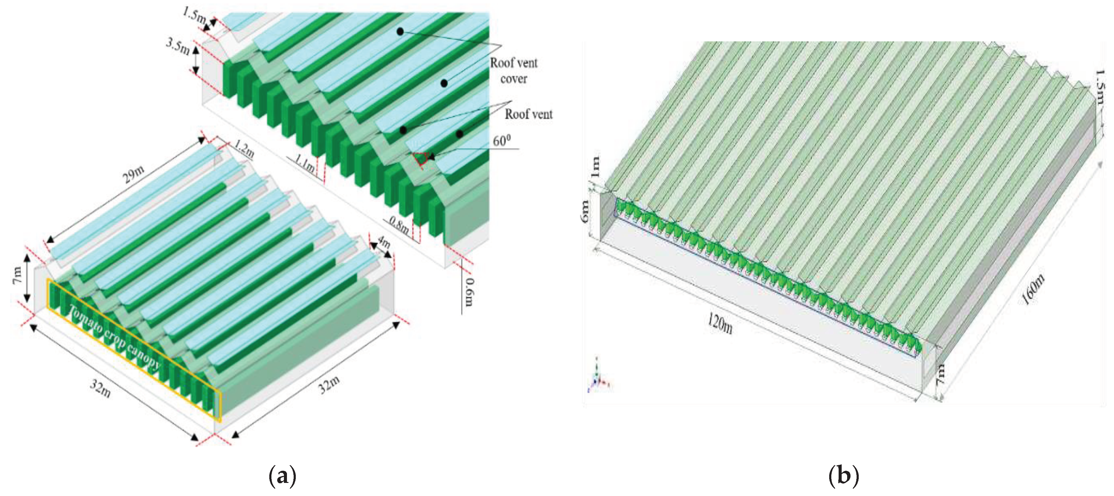
To model the target 2 ha greenhouse, a standard 0.1 ha, 8 span Venlo greenhouse, designed for 19 tomato crop rows was adopted from ministry of food, agricultural, Forestry and Fisheries of Korea structural design standard of 1999, and upscaled its horizontal dimensions (32 m by 32 m) by a factor of 3.5 in width and 5 in length to form a 30 span 2 ha large-scale model. To have more than one grid cell across the plant canopy rows during model discretization, 3 plant rows in the standard greenhouse were simplified into one row in the model greenhouse. Natural ventilation operation conditions were considered, with only roof top ventilation. The roof vent cover opening angle was 60, to represent average operation conditions during summer season.
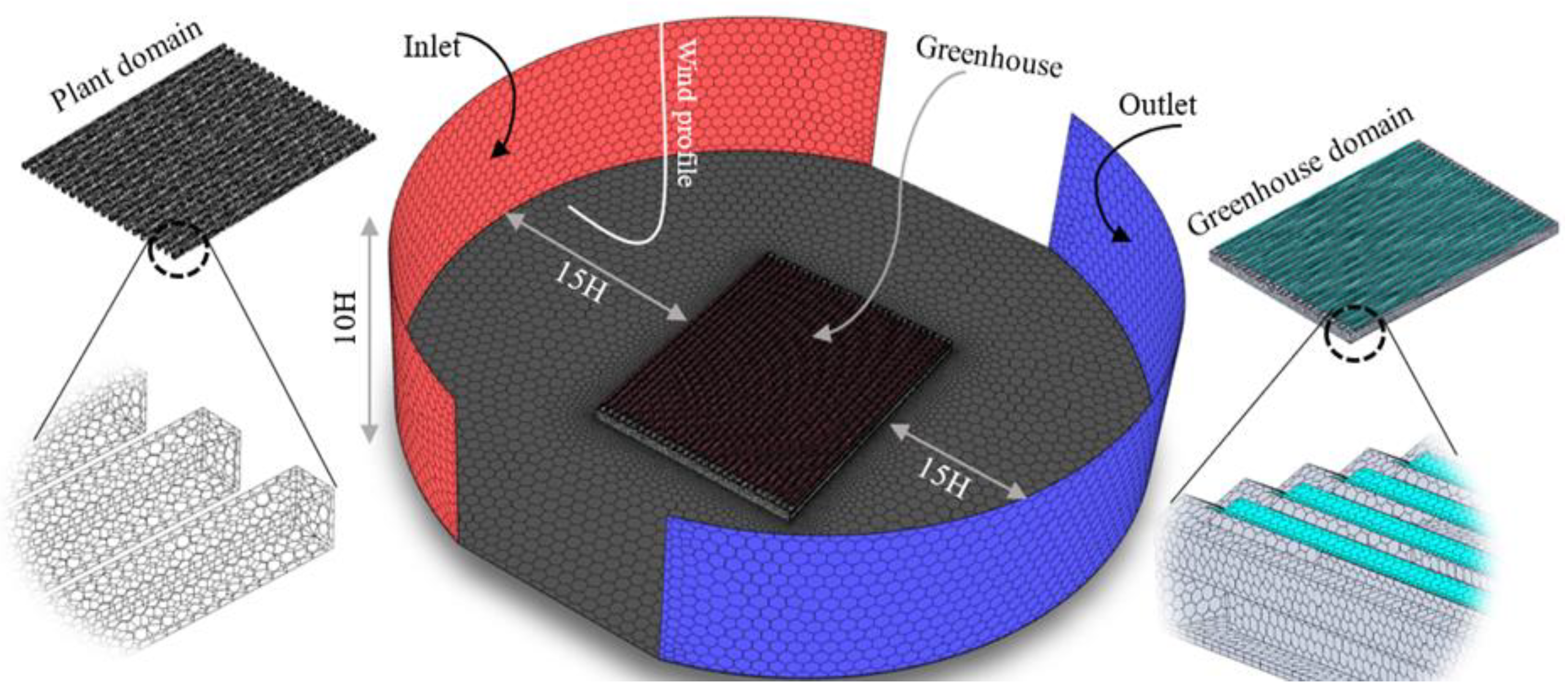
The modeling process was implemented in Ansys Space claim (Ver. 2022 R2, USA) software to make the 3D CAD model for the 2 ha greenhouse. Figure 2 shows a schematic representation of the small-scale standard greenhouse and the developed 3D 2 ha greenhouse model. For simulation purposes, the greenhouse external environment was developed following the methods described in Materials and methods Section 2.3. The overall computation domain was cylindrical with a radius of 105 m and a height of 70 m ( See Figure 4).
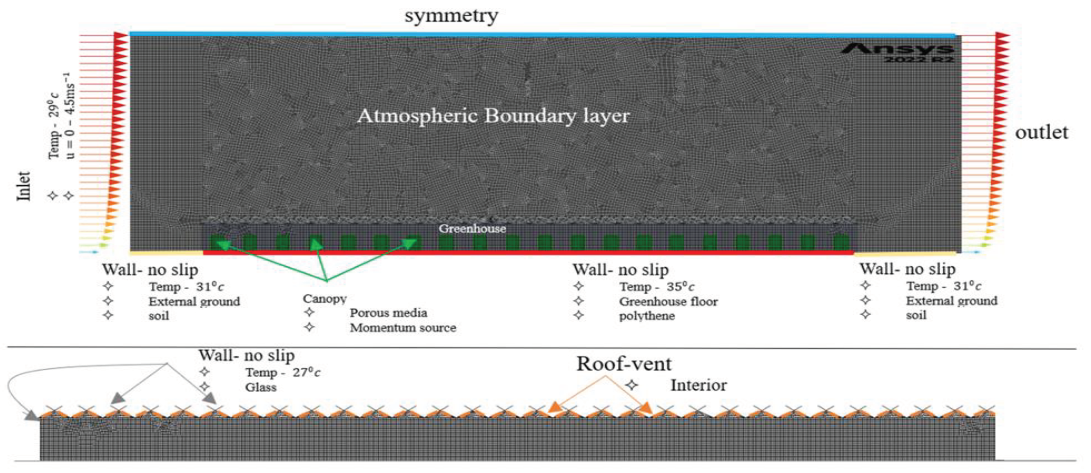
To make the 2D CFD model, the model was sectioned along the center of the greenhouse across the crop canopy in the vertical plane. The 2D cross section model domain was discretized into computational grids using Ansys Meshing software. The 2D model was used to generate the reference data set and GIT study. For reference data generation, a fine grid of 0.2m resolution model was developed. For GIT study, several CFD models with coarse grid resolutions of 0.3m, 0.4 m 0.5 m, 0.6 m, 0.7 m, 0.8 m, 1.0 m, 2.0 m, and 3.0 m were developed for optimal grid determination. The CFD models were simulated in Ansys Fluent software where the model boundary conditions, and crop canopy models were implemented. The 2D simulations were steady state regime and simulations were run until the preset convergence criteria was met. The 0.2 m grid 2D model boundary conditions are illustrated in Figure 3, and the Ansys fluent CFD settings, operating conditions and models used are shown in Table 5.
To make the 3D CFD model, the 2-ha greenhouse model was discretized using the optimal grid resolution (0.8 m) determined in the GIT process from the 2D simulations. The model was made up of 5 million polyhedral cells, 0.8m size in plant canopy and greenhouse with a growth rate 1.2 to the external environment Figure 4. The model was first simulated in steady state until convergence and then switched to transient regime for TGD simulation. The transient simulation flow time was 10 minutes with 1 second time steps using Carbon-dioxide gas as the trace gas. The boundary condition and CFD settings were like those used in the 2D simulation. The material properties and values used for both 2D and 3D models are shown in Table 2.
Figure 3. (a) 0.1 ha standard Venlo greenhouse with 8 spans and (b) modeled large scale 30 span 2 ha Venlo greenhouse.
Preprints 79290 g003
Figure 4. 0.2m grid size computation grid, boundary conditions and imposed values for 2D simulation.
Preprints 79290 g004

2.7.3. Model verification procedure

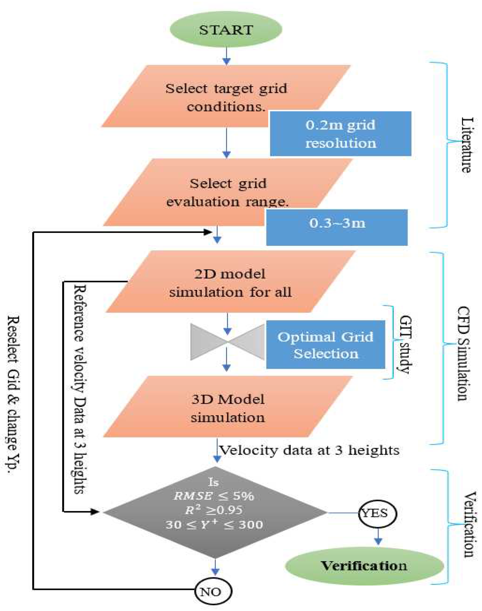
Model verification was performed using GIT, Y+, R2 and RMSE methods. Based on the reviewed literature about greenhouse CFD modeling, grid resolution of 0.2 m and the RNG k-ε turbulence model have been reported optimal for designing greenhouse CFD model through validation with field data. In this study, 0.2 m grid resolution and RNG k-ε turbulence model were used to design the 2D model for reference data generation that was considered as baseline for model verification judgment. GIT was used to determine the minimum grid resolution required to obtain a converged and accurate solution. This was to ensure that the numerical solution is accurate and reliable, while minimizing computational costs. Wall Y+ was used to resolve the near wall boundary layer resulting from the high solution gradient at the model walls. Model verification was performed by comparing air velocity results from the 2D 0.2 m grid resolution model to results from 3D model simulation. The model was considered verified when the following conditions were satisfied: R2 ≥ 0.95, RMSE ≤ 5% and 30 ≤ Y+ ≤ 300. The procedure used in model verification is shown in Figure 5. It involved 6 major steps described below.
  • Identifying a recommended grid size. 0.2 m grid resolution and RNG k-ε turbulence model were adapted from literature and used in 2D simulation to generate a reference set of data.
  • Selection of grid resolution range for GIT study. With reference to reviewed literature, a range between 0.3 m to 3 m resolution was selected for optimal resolution determination.
  • 2D simulation. The 0.2 m grid resolution model was simulated to generate reference air velocity data. Coarse grid resolution models were also simulated, and average velocity data was extracted at 0.7 m, 2.2 m, and 3.5 m heights.
  • GIT study. The average air velocity data for all the coarse grid resolutions was compared to the reference data. The grid resolution above, which the results started to diverge away from the reference data was selected as optimal grid and tested in 3D model.
  • 3D simulation. The selected optimal grid was used to make the 3D model and simulated with the same boundary condition with the 2D simulation. Average air velocity was extracted at the study heights and wall Y+ was checked.
  • Verification. The 3D results were statistically compared to the reference data by evaluating the R2, RMSE and checking Y+. Near wall mesh refinement using the first layer height of 0.04 m was used to iteratively adjust wall Y+ value into the target range. When the verification procedure was all satisfied, natural ventilation, micro-environment distribution and flow pattern were analyzed to assess the performance of the designed model.

2.8. Analysis procedure

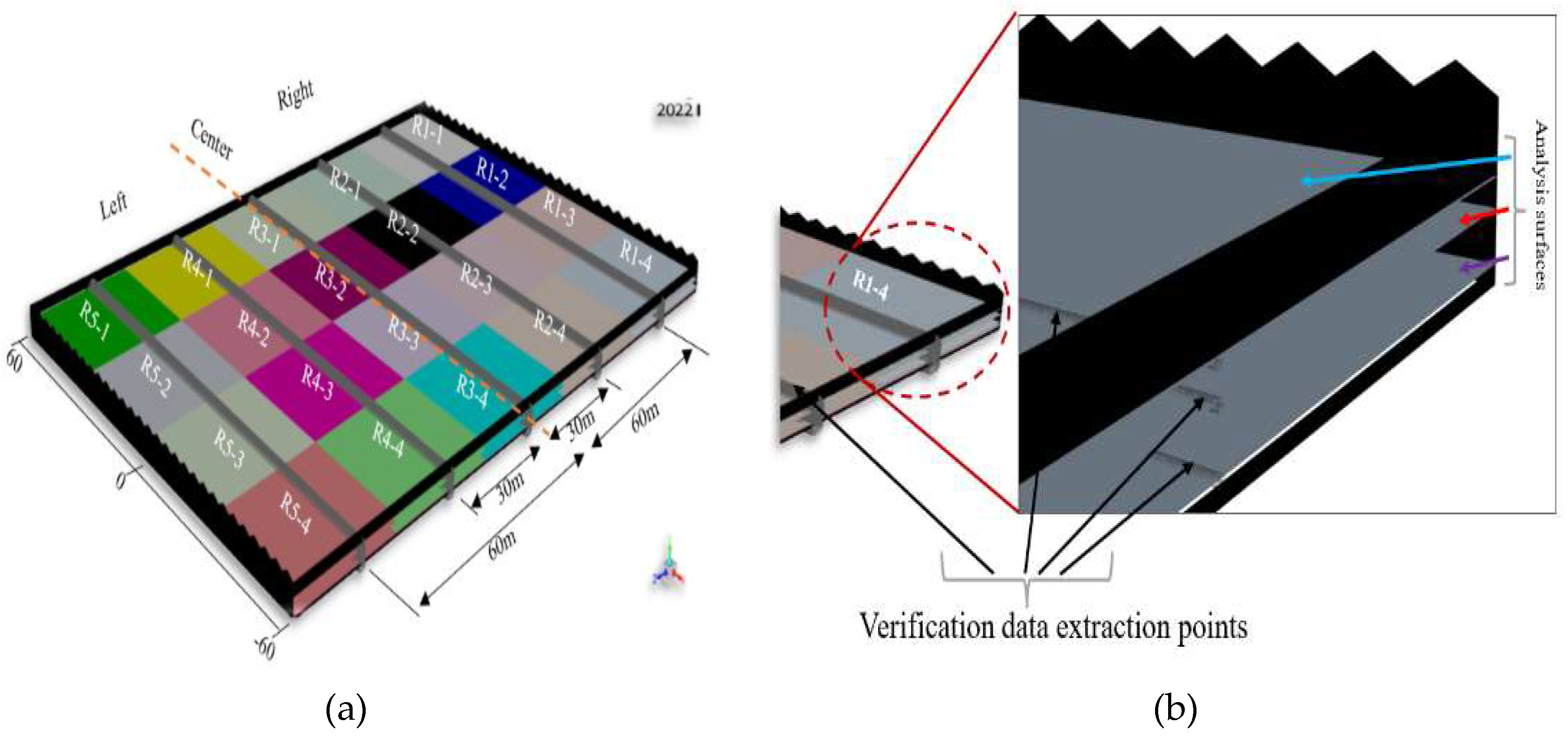
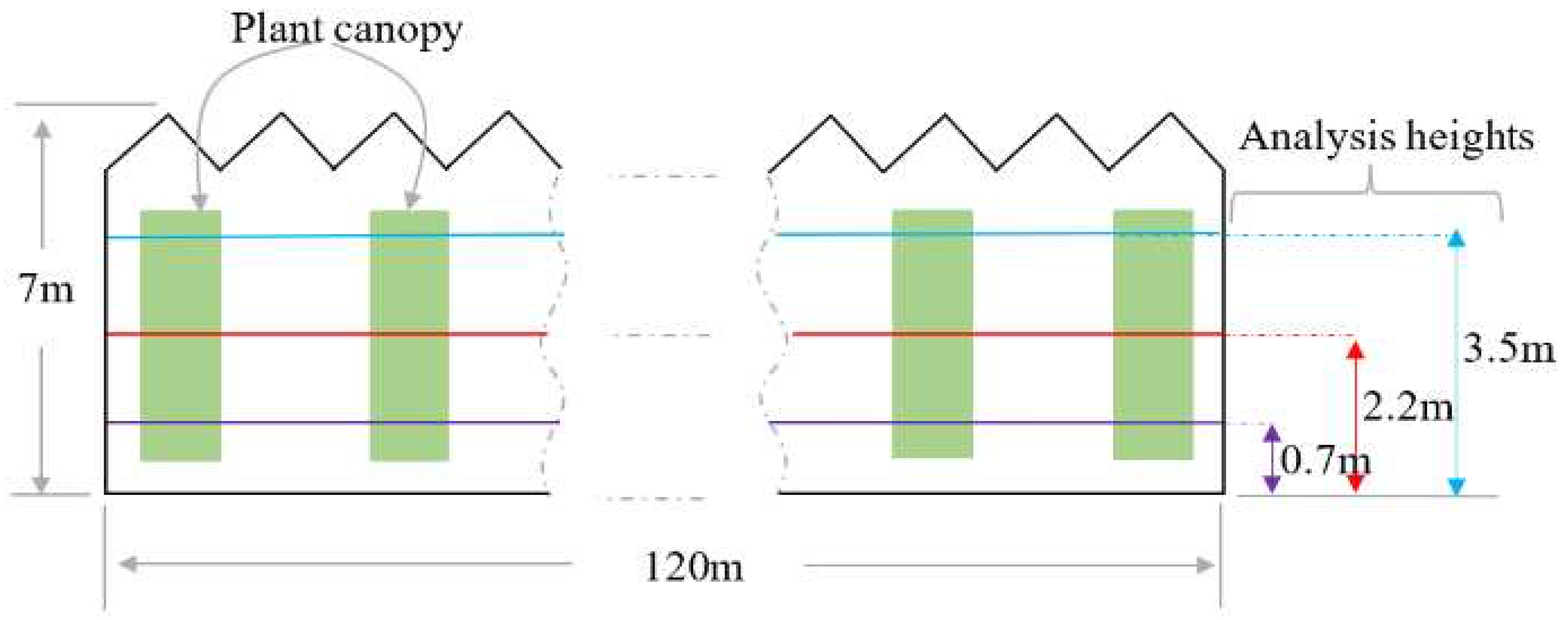
To analyze the local ventilation efficiency, the greenhouse was subdivided into 20 analysis regions (5 by 4), and each analysis region was identified by a unique code in the form R(RC) based on their row and column positions in the greenhouse (Figure 6a). Parameters were also analyzed according to height, at 0.7 m, 2.2 m, and 3.5 m heights within the crop canopy from the ground (Figure 7). In the model accuracy verification stage, simulated data was extracted from 1,000 points within the model at the three study heights from the center of the greenhouse for both the reference data in the 2D model and 3D verification model (Figure 6b). Velocity distribution in 3D greenhouse was also analyzed at 30 m and 60 m from the center of the greenhouse to both sides along the length of the greenhouse at all the 3 analysis heights (Figure 6a).

3. Results and discussion

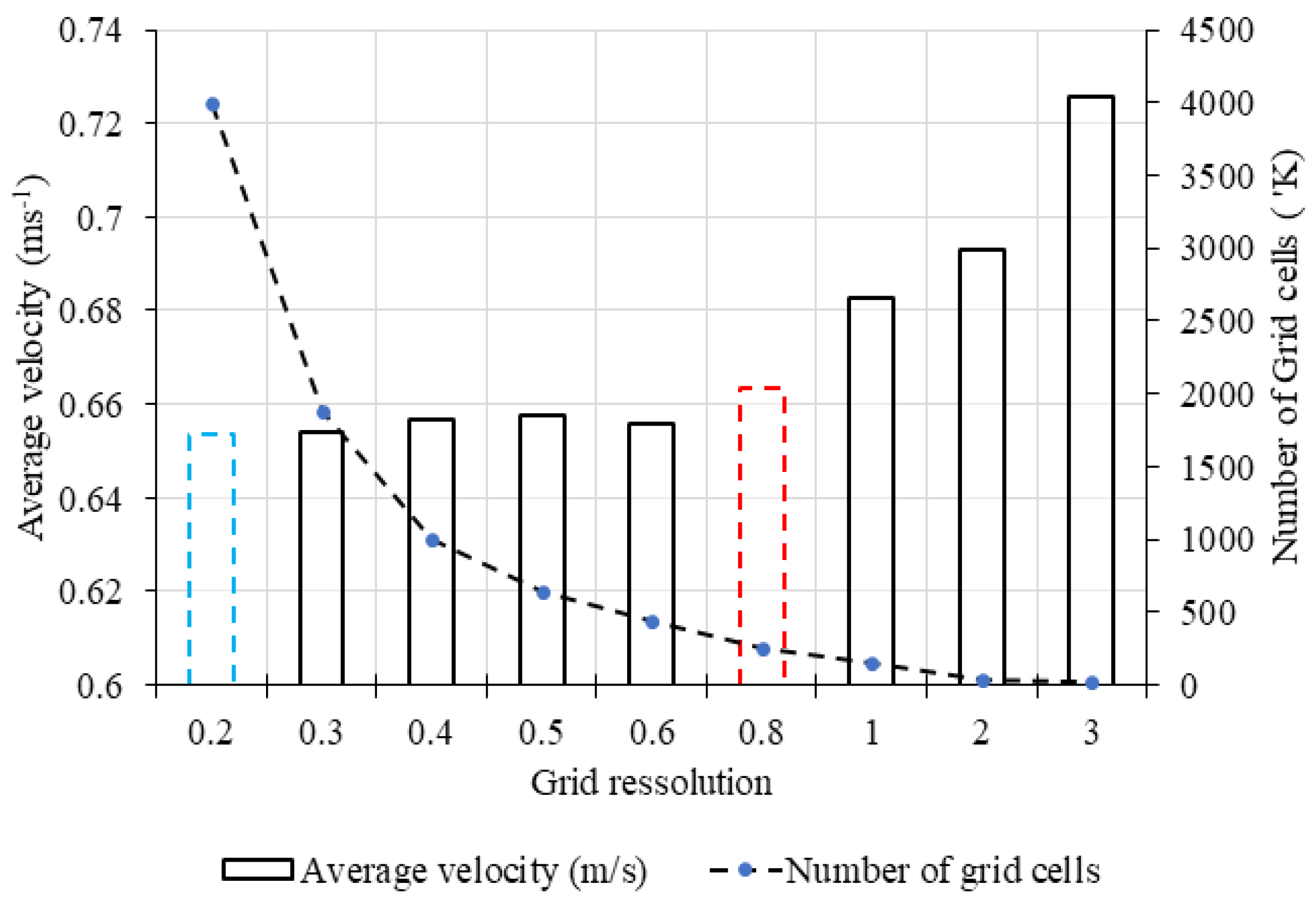
For the reference grid resolution model, the average air velocity in both the greenhouse and plant domains was 0.654 m·s-1 (Figure 26). This value is close to 0.58 m·s-1 reported by [30] in 1 ha greenhouse with tomato canopy. Generally, average greenhouse air velocities have been reported to range between 0-1.5 m·s-1 for natural ventilation regime. The generated reference set of data was hence deemed in range with the validated values from literature and could be used as baseline for the 3D model accuracy verification. The air velocity results based on larger grid resolutions between 0.3 m-0.8 m showed no significant difference compared to 0.654 m·s-1 obtained from simulation with the reference grid size. For grid sizes larger than 0.8 m, the average air velocity diverged away from the reference value. 0.8 m grid size was hence selected as the optimal grid and considered for statistical comparison with the reference data in the 3D model.
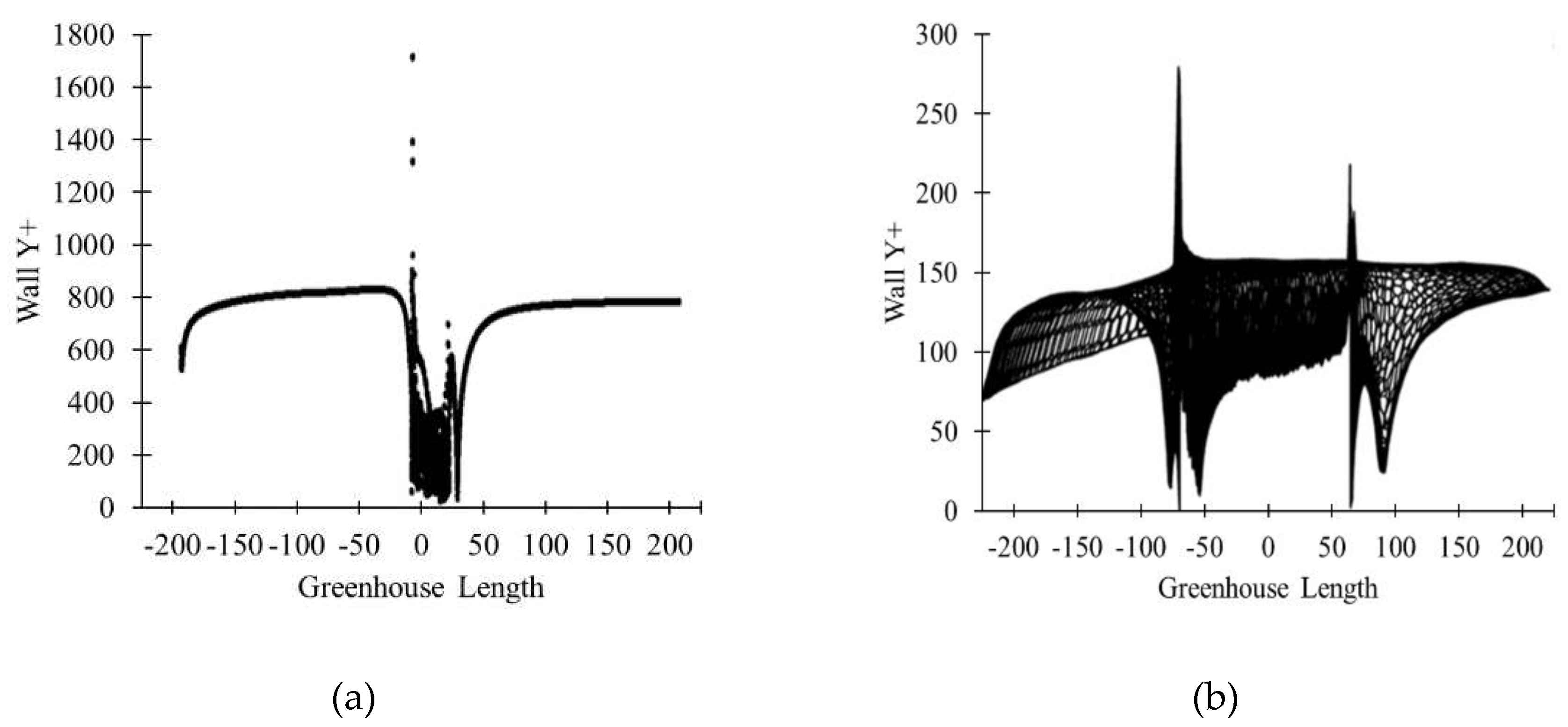
The maximum initial wall Y+ value was 1,800 on the windward side of the greenhouse cover material (Figure 9). The average wall Y+ value was determined to be 600, which was far outside the target range. After evaluation, it was determined that a first layer height of 0.04 m would be suitable to reduce the Y+ value within the required range for accurate resolution of the boundary layer. This adjustment resulted in a maximum wall Y+ value of 270 in the 3D model, which satisfied the requirement for the RNG k-epsilon turbulence model with enhanced wall functions. To refine the near wall zone, all the cells were refined using four inflation layers, with the first layer having a height of 0.04m and a growth rate of 1.2 towards the external domain. This refinement only increased the total number of cells by 120,000. As a result, the overall 3D computational domain consisted of a grid with 5.5 million cells. Average after statistical comparison between the velocity results from 3D 0.8 m.
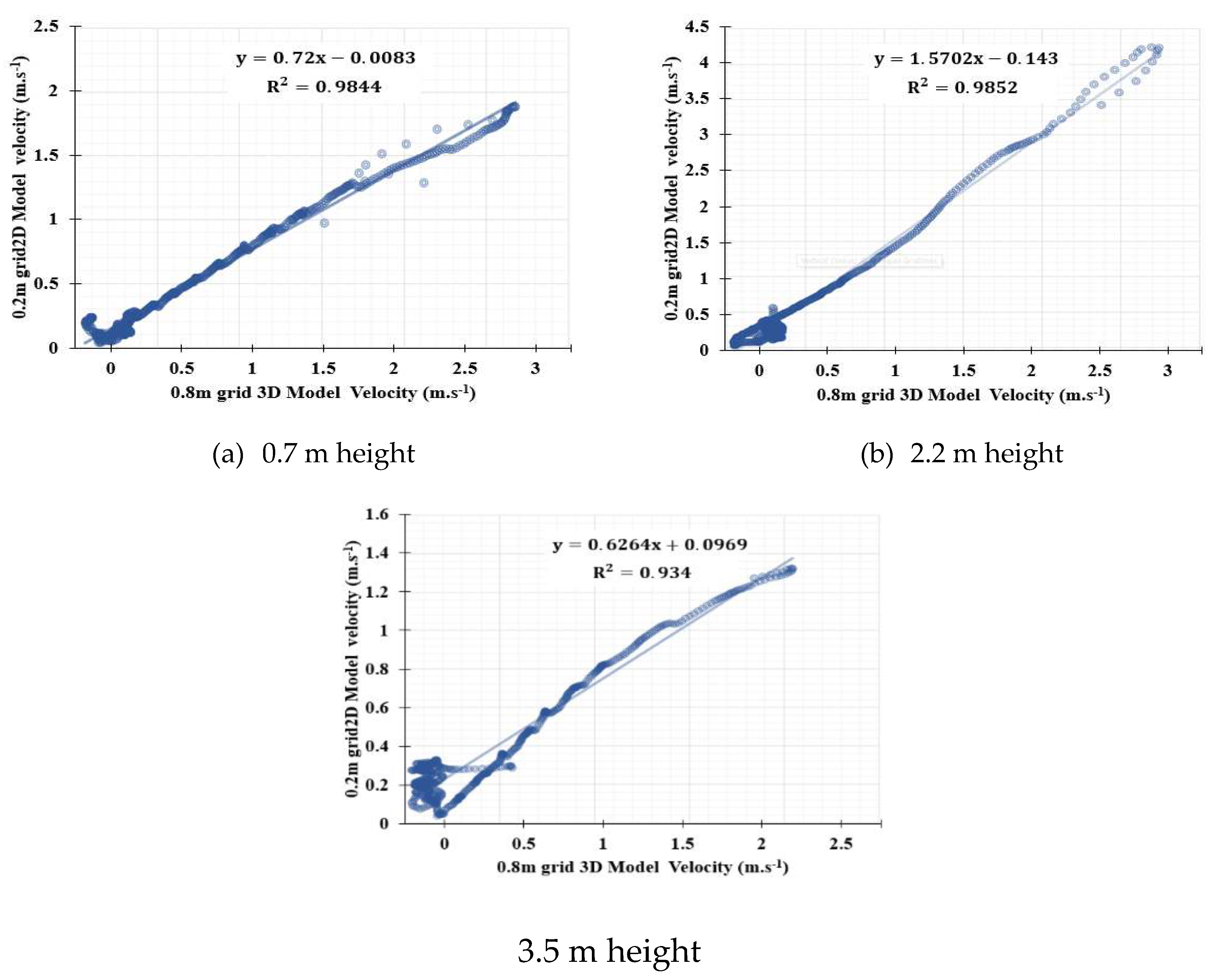
After statistical comparison between the velocity results from 3D 0.8 m grid model simulation to the 2D reference model results, the R2 values were 0.9844, 0.9853 and 0.934 while RMSE values were 5.61, 3.96 and 2.20 at 0.7 m.
2.2 m and 3.5 m heights respectively (Table 4). Highest R2 value (0.9844) and highest RMSE value (5.61) were observed at 0.7 m height. The lowest R2 and RMSE values (0.934 and 2.2) were observed in the 3.5 m height (Figure 10). This could be due to the effect of direct influence of the external wind to the local air flow at 3.5 m in the greenhouse through the roof window vents. The average R2 and RMSE for all the 3 analysis heights were 0.968 and 3.923% respectively, which both meet the verification conditions.
Table 3. Material physical properties and value used for 2D and 3D simulation models.
Parameters (units) Material Value
Refractive index Polythene (floor cover) 0.8
Thickness (mm) Cover glass 4.0
Density (kgm-3) Soil 1900
Glass 2700
Specific heat (J.kg-1.0C-1) Soil 2200
Glass 840
Thermal conductivity (W.m2. 0C) Soil 2.0
Glass 0.78
Absorption coefficient Soil 0.5
Glass 0.1
Scattering coefficient Soil 1.0
Glass 0
Refractive index Soil 1.0
Glass 1900
Table 4. 3D/2D simulation CFD software settings, models, and operating conditions.
Variable CFD Solver setting
Time Steady state (3D, 2D) / Transient state(3D)
Solver Pressure based solver
Numerical algorithm SIMPLE algorithm
Discretization Second order
Operating pressure 101,325 pa
Gravity 9.81 (m·s-2)
Air density Variable (ideal gas)
Air viscosity 1.78994 (kg·m-1·s-1)
Turbulence RNG κ-ε
Empirical wall function Enhanced wall functions
Table 5. Analysis height based statistical indices from comparing 0.8m grid size average air velocity results to the reference data set generated from 0.2m grid size.
Height R- Square RMSE
0.7 0.9844 5.61
2.2 0.9852 3.96
3.5 0.934 2.2
Average 0.968 3.923

Aerodynamic analysis of 3D greenhouse model

Internal air velocity profile and air flow pattern.

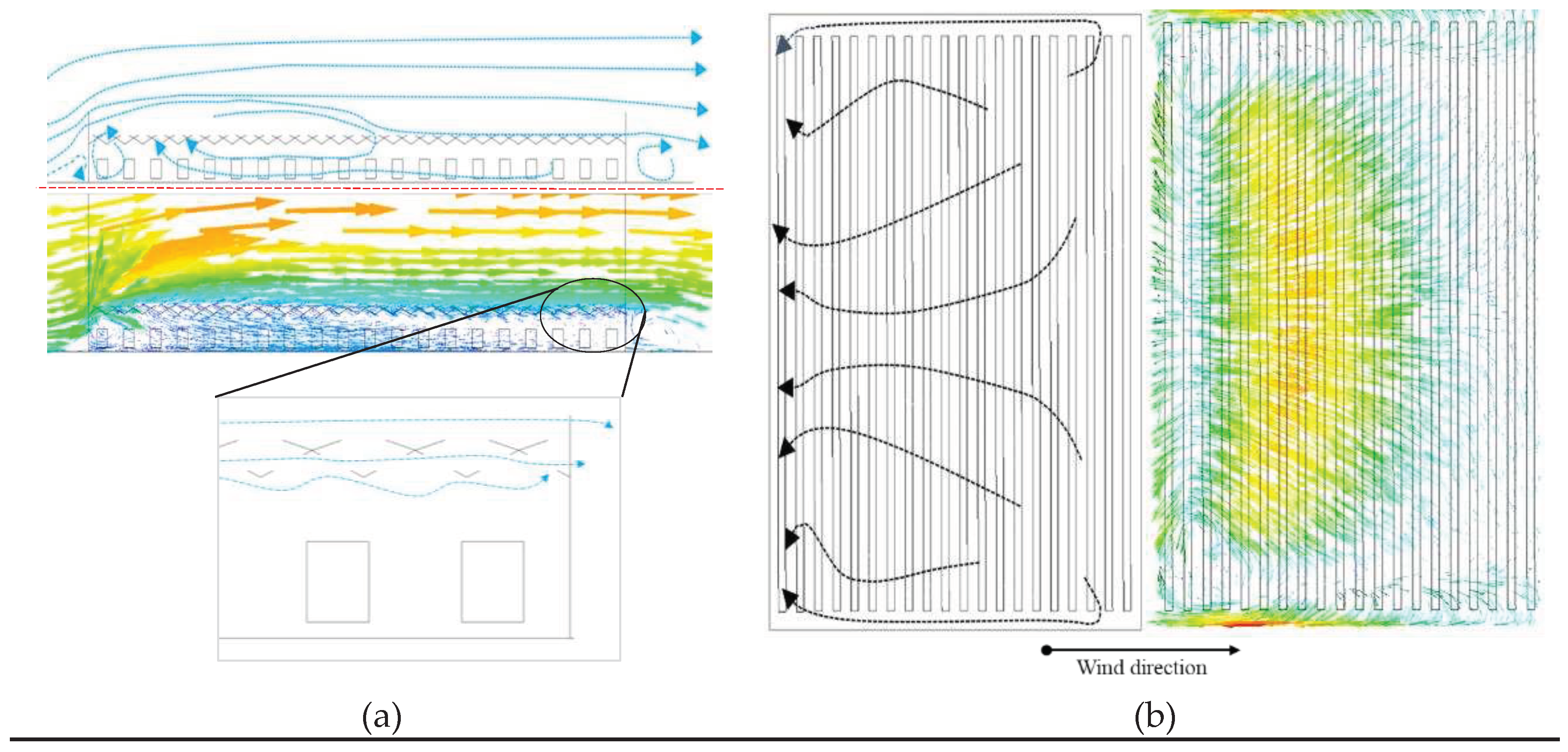
The analysis of greenhouse internal and external air flow patterns revealed that only a small fraction of the external air streams entering the greenhouse through the roof windows reached the interior. Instead, the flow streams continued through consecutive windows and exited back to the outside (Figure 13). Most of the streams that entered the greenhouse were observed in the central region, flowing towards the leeward side where the pressure was lower. Conversely, no streams were observed entering the greenhouse in regions of high pressure on the leeward side (Figure 14). This flow pattern induced slow air speed in the plant canopy in the opposite direction, which explains the observed velocity distribution.
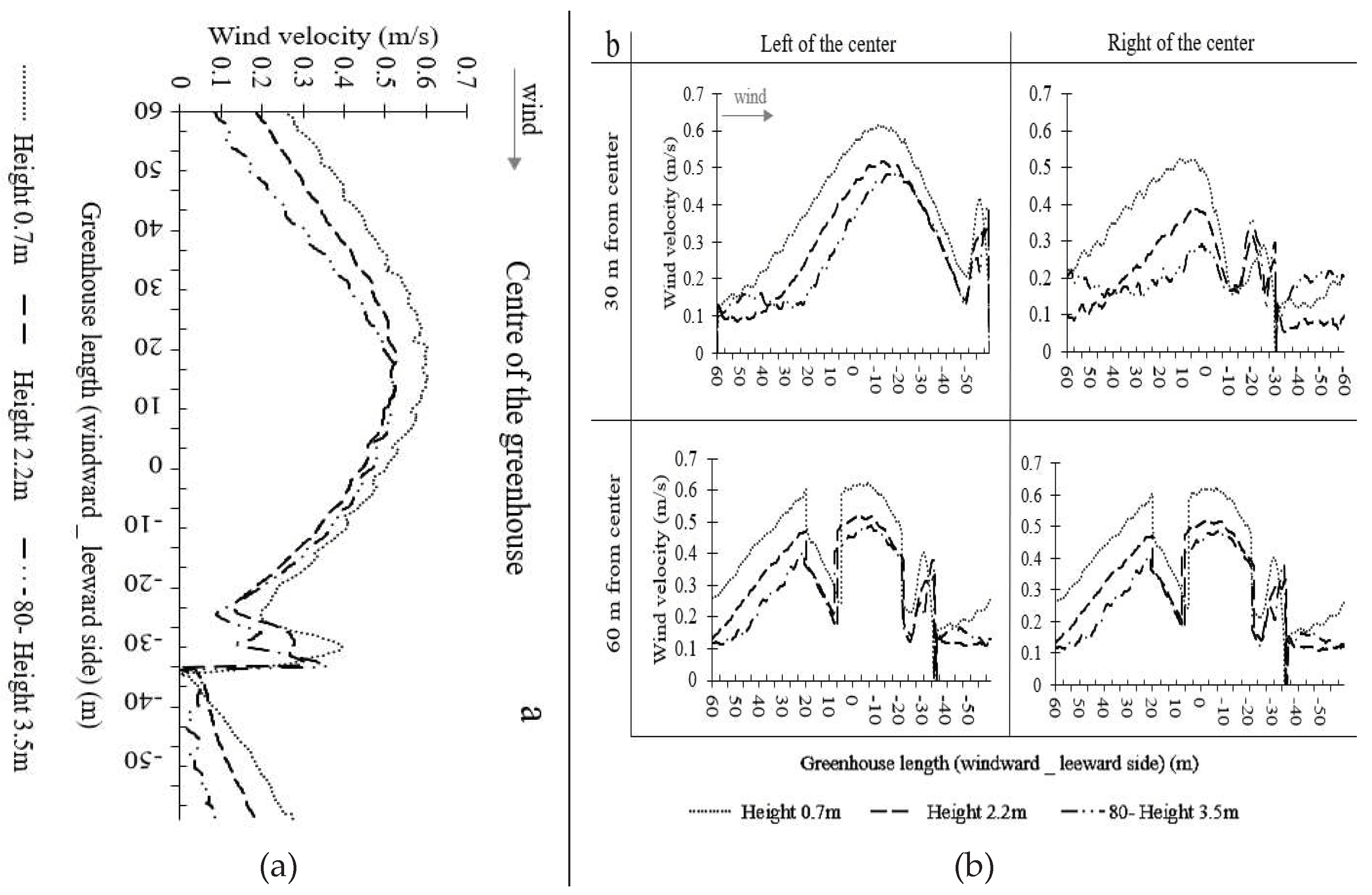
The air velocity profile at 30 m from the center, both to the right and left sides were closely like that at the center, with the highest velocity occurring at a height of 0.7m and the lowest velocity at a height of 3.5m. However, at 60m from the center, significant variations in the velocity profiles were observed, with velocities sharply dropping to 0 m/s at certain points (Figure 13). This result shows that the distribution of wind velocity inside a 2-ha greenhouse varies with horizontal distance from the center.

Internal environmental distribution
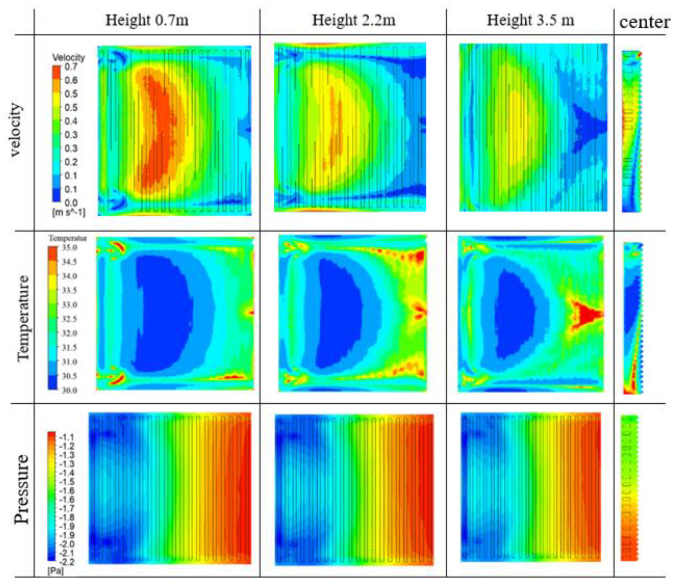
The temperature inside the greenhouse ranged from 30 to 35°, representing a temperature rise of 6 degrees above the ambient temperature. The temperature distribution exhibited a similar pattern to that of the air velocity, with higher temperatures observed in the center of the greenhouse and gradually decreasing towards the walls.
The internal pressure ranged from -2.2 to -1.1 pascals. In terms of air velocity, the highest values were recorded at a height of 0.7 m, reaching a maximum of 0.7 m.s-1. The velocity decreased with increasing height, with the highest velocities at 2.2 m and 3.5 m heights measuring 0.6 m.s-1and 0.5 m.s-1, respectively. The lowest velocity observed at all heights was 0.2 m.s-1. regions with air velocity below 0.2 m.s-1are referred to as dead zones, characterized by a significant.
Temperature increase and lowest ventilation efficiency (Figure 12b).
This flow distribution can be attributed to insufficient direct entry of air streams from the outside into the greenhouse. The air movement inside the greenhouse was primarily a result of the vacuum created at the top of the greenhouse by the higher speed external wind streams, leading to an internal negative pressure. The resultant vertical velocity profiles from the windward side of the greenhouse at the center, 30 m to the left, and 30m to the right are illustrated in Figure 12. Similar velocity distribution profiles and trend have been reported in several previous research.
Figure 12. CFD results of (a) internal velocity vectors and air flow pattern at the center; (b) horizontal velocity vectors and air flow pattern at 2.2 m height.
Preprints 79290 g012
Figure 13. Vertical velocity profiles at the center and at 30 & 60m from center to left and right from the center along the length of the greenhouse.
Preprints 79290 g013
Figure 14. Velocity, temperature, and pressure contours at the center and different analysis heights.
Preprints 79290 g014

Ventilation efficiency.

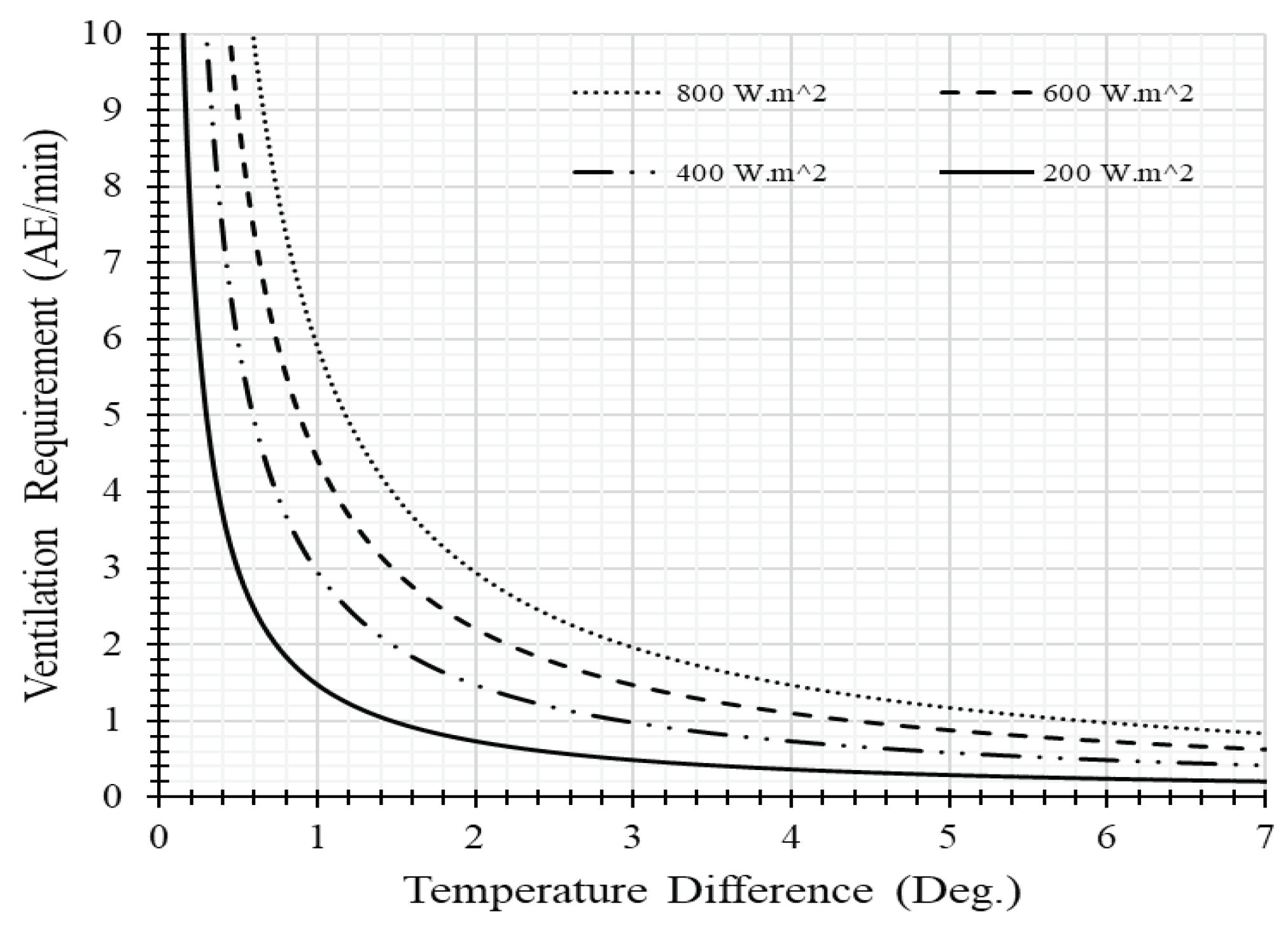
The ventilation requirement increased as the external radiation levels increased and decreased with an increase in the desired temperature difference (∆T). In the summer season, where the average solar radiation was approximately 800 W.m2, the current model greenhouse required approximately 6 AER (min-1) to maintain a 1℃ temperature difference (Figure 16). This value is lower than the reported value of 7.5 AER (min-1) for a 0.1 ha Venlo greenhouse under the same weather conditions, as stated by Lee et al. (2018). The variation in these reported values can be attributed to the differences in the greenhouse volumes considered in the two studies (0.1 ha and 2 ha). Furthermore, the previous model did not consider the effect of the crop canopy, which may also contribute to the observed differences in ventilation requirements.
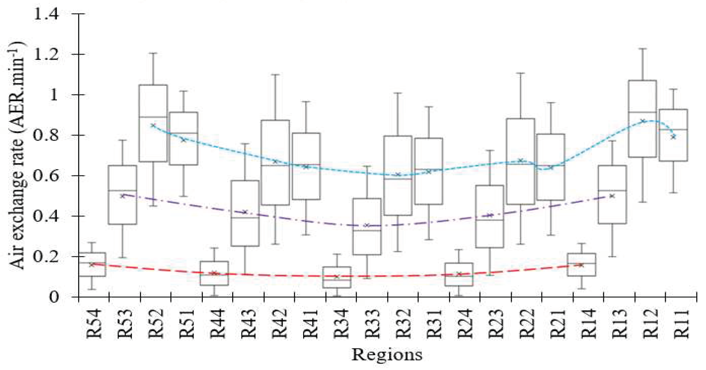
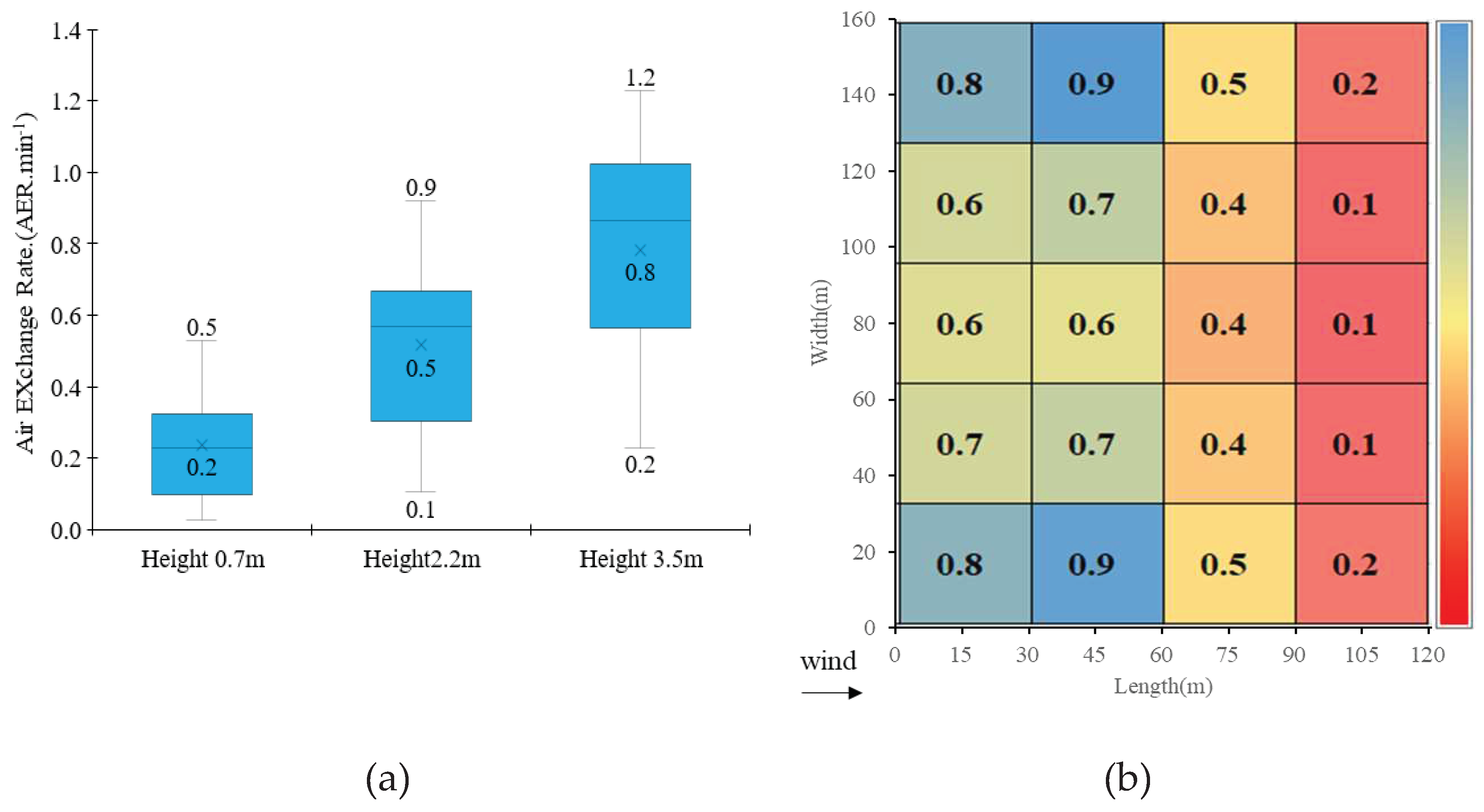
Ventilation efficiency was assessed by computing the local distributions of tracer gas concentrations within the greenhouse. The time-dependent variation of tracer gas concentration at a height of 2.2m within the greenhouse and plant canopy, at flow times of 2, 4, 6, and 10 minutes, is illustrated in Figure 15. The concentration at a flow time of 10 minutes was used to evaluate the ventilation efficiency and its spatial distribution. As a result of analyzing the ventilation efficiency by height, it was observed that the efficiency increased with height (Figure 16). The lowest average air exchange rate (AER) was found to be 0.2 min-1 at a height of 0.7m, with the lowest standard deviation. Interestingly, despite the highest air velocities being observed at a height of 0.7m, the ventilation efficiency was the lowest at this height. Conversely, the reverse trend was observed at a height of 3.5m. These results suggest that the air at the bottom of the greenhouse had a higher mean-age-of-air (MAA) due to the induced internal pressure distribution resulting from the crop canopy effect and the flow pattern at the roof window. The distribution of ventilation efficiency among the analysis regions revealed three distinct clusters, as indicated by the dotted lines in Figure 18. Regions that were furthest from the windward side exhibited the lowest air exchange rates, with an average of 0.2 min-1. Generally, ventilation efficiency exhibited a decreasing trend as the distance from the windward side increased.
Figure 15. Variation of ventilation requirement the internal-external temperature difference at different external solar radiations.
Preprints 79290 g015
Figure 16. Simulated distribution of carbon-dioxide gas concentration inside the greenhouse at various flow times.
Preprints 79290 g016
Figure 17. Ventilation efficiency evaluation by analysis heights.
Preprints 79290 g017
Figure 18. (a) Ventilation efficiency distribution by analysis heights, (b) overall local ventilation efficient distribution by regions.
Preprints 79290 g018
Figure 19 shows a distinct valley pattern observed from all the dotted lines at the center. This indicates that ventilation efficiency decreases as one moves deeper into the crop canopy from the side walls of the greenhouse. Regions located purely within the plant canopy form the bottom points of these valleys. This can be attributed to the drag force effect of the crops on the airflow and the porous nature of the crop canopy implemented in the model.
The overall spatial distribution of ventilation efficiencies is depicted in Figure 20, considering the analysis regions. The distribution behavior is correlated with the pressure distribution, as the lowest ventilation efficiencies are observed in regions with the highest pressure. The overall ventilation efficiency of the greenhouse was calculated to be 0.51 AER (min-1). In a study by Lee et al. (2018) on a plant-less 8-span (0.1 ha) Venlo greenhouse with only roof windows open, ventilation efficiencies of 0.28 and 0.58 AER(min-1) were reported for external wind speeds of 2.5 m.s-1and 5.5 m.s-1, respectively. The current model, on the other hand, considered an external wind speed of 3 m/s and a 2 ha greenhouse with a tomato canopy. Due to the inverse impact of the crop canopy and greenhouse volume on ventilation efficiency, these two results seem to exhibit disproportionate differences.
The current model considered summer conditions, with an average daily solar radiation of 800 W.m-2. For proper tomato crop growth in a naturally ventilated greenhouse, it is recommended to maintain a maximum temperature difference of 5 degrees Celsius. To satisfy the ventilation requirement (5-degree temperature difference at 800 W/m2), the model requires an air exchange rate of 1.2 AER (min-1) (Figure 21). The simulated ventilation efficiency of 0.51 AER (min-1) indicates that a naturally ventilated 2 ha greenhouse under reclaimed land weather conditions does not meet the ventilation requirements for tomato cultivation during the summer season. At an air exchange rate of 0.51 AER (min-1), it can be observed that the greenhouse can only satisfy the recommended natural ventilation conditions when the external radiation is 200 m.s-1 (point a). When the external radiation is 400 m.s-1, the simulated air exchange rate meets the requirement but cannot maintain the temperature difference above 5 degrees Celsius (point b). In summary, the 2 ha Venlo greenhouse under tomato cultivation, with an external wind speed of approximately 3 m/s, exhibits internal and external air flow patterns resulting in air velocities ranging from 0 to 0.7 m/s, temperatures ranging from 30 to 35 degrees Celsius, an average ventilation rate of 0.51 AER (min-1) with a standard deviation of 0.25, and pressures ranging from -2.2 to -1.1 pascals within the crop canopy. Most regions have wind velocities below 0.2 m/s, with higher temperatures at least 5 degrees Celsius higher than the external temperature. These results describe a highly heterogeneous internal microenvironment and an inefficient natural ventilation system for tomato cultivation. Under these conditions, modifications to the ventilation system are required to meet the appropriate growth conditions for tomato crops.

4. Conclusions

Understanding the air exchange mechanisms between the inside and outside of greenhouses is crucial for evaluating the internal microenvironment and the interaction with the crop canopy. CFD models that consider the crop canopy, external wind characteristics, and greenhouse structure provide a realistic representation of the entire greenhouse volume, even at a local distribution level. However, the design and validation of these CFD models are critical steps before they can be used for detailed analysis and making commercial decisions. Developing CFD models for large-scale greenhouses and greenhouse complexes can be challenging due to the limited availability of field data for validation and the computational capabilities required for model simulations. In this study, it has been demonstrated that by using previous research results as a baseline and incorporating improved Grid Independence Test (GIT) and Wall Y+ methods, an efficient procedure for design optimization, accuracy verification, and grid reduction in large-scale CFD models can be developed and adopted. Even without extensive field data, these approaches yield accurate results that are statistically evaluated, while significantly reducing the number of grid cells. This makes it feasible to model very large greenhouse complexes. Specifically, it has been shown that a grid resolution of 0.8 m within the greenhouse and plant domain is sufficient to obtain closely accurate results compared to using a finer grid size of 0.2 m. The accuracy verification results yielded low RMSE values (as low as 3.9%) and high R2 values (0.968), resulting in a 38% reduction in the number of grid cells. This demonstrates the effectiveness of the proposed approach in achieving accurate results while reducing computational requirements. Through the testing of these approaches, it has been observed that the external wind directly influences the airflow direction inside the greenhouse, leading to a negative pressure environment. This induces a stronger wind-wise air current above the crop canopy and a slow reverse flow inside the crop canopy, which aligns with findings from previous studies. Furthermore, it is evident that greenhouse size and canopy have a significant impact on the overall ventilation requirement and efficiency. For a 2 ha Venlo greenhouse built on reclaimed lands in Korea, when the incoming wind is perpendicular to the roof windows, the average ventilation efficiency is estimated to be 0.51 air exchanges rate (min-1), while the ventilation requirement is 1.2 AER (min-1). These results indicate that the natural ventilation system of the greenhouse does not meet the requirements for the summer season, emphasizing the need for modifications or alternative ventilation strategies to achieve appropriate conditions for tomato cultivation. These results will be used to develop a large-scale greenhouse complex model with multiple greenhouses to analyze the effect of eternal wind variation to internal air flow and distribution of crop growth factors according to greenhouse location in the complex.

Acknowledgments

This work was carried out with the support of "Cooperative Research Program for Agriculture Science & Technology Development (Project No.: PJ01558601202201)" Rural Development Administration, Republic of Korea.

References

  1. Misra, A.K. Climate change and challenges of water and food security. Int. J. Sustain. Built Environ. 2014, 3, 153–165. [Google Scholar] [CrossRef]
  2. Gruda, N.; Bisbis, M.; Tanny, J. Impacts of protected vegetable cultivation on climate change and adaptation strategies for cleaner production – A review. J. Clean. Prod. 2019, 225, 324–339. [Google Scholar] [CrossRef]
  3. Akrami; et al. Study of the effects of vent configuration on mono-span greenhouse ventilation using computational fluid dynamics. Sustain. 2020, 12. [Google Scholar]
  4. Lin, D.; Zhang, L.; Xia, X. Hierarchical model predictive control of Venlo-type greenhouse climate for improving energy efficiency and reducing operating cost. J. Clean. Prod. 2020, 264, 121513. [Google Scholar] [CrossRef]
  5. Villagran, E.; Bojacá, C.; Akrami, M. Contribution to the sustainability of agricultural production in greenhouses built on slope soils: A numerical study of the microclimatic behavior of a typical colombian structure. Sustain. 2021, 13. [Google Scholar] [CrossRef]
  6. Lee, S.-Y.; et al. Analysis of Natural Ventilation Rates of Venlo-type Greenhouse Built on Reclaimed Lands using CFD. J. Korean Soc. Agric. Eng. 2015, 57, 21–33. [Google Scholar]
  7. Van, E.J. (wageningen university Henten, Greenhouse climate management : An optimal control approach. 1994.
  8. Yang, S.H.; Rhee, J.Y. Utilization and performance evaluation of a surplus air heat pump system for greenhouse cooling and heating. Appl. Energy 2013, 105, 244–251. [Google Scholar] [CrossRef]
  9. Ozgener, O.; Hepbasli, A. An economical analysis on a solar greenhouse integrated solar assisted geothermal heat pump system. J. Energy Resour. Technol. Trans. ASME 2006, 128, 28–34. [Google Scholar] [CrossRef]
  10. Canakci, M.; Emekli, N.Y.; Bilgin, S.; Caglayan, N. Heating requirement and its costs in greenhouse structures: A case study for Mediterranean region of Turkey. Renew. Sustain. Energy Rev. 2013, 24, 483–490. [Google Scholar] [CrossRef]
  11. Campen, J.B.; Bot, G.P.A. Determination of greenhouse-specific aspects of ventilation using three-dimensional computational fluid dynamics. Biosyst. Eng. 2003, 84, 69–77. [Google Scholar] [CrossRef]
  12. Benni, S.; Tassinari, P.; Bonora, F.; Barbaresi, A.; Torreggiani, D. Efficacy of greenhouse natural ventilation: Environmental monitoring and CFD simulations of a study case. Energy Build. 2016, 125, 276–286. [Google Scholar] [CrossRef]
  13. Ganguly, A.; Ghosh, S. Model development and experimental validation of a floriculture greenhouse under natural ventilation. Energy Build. 2009, 41, 521–527. [Google Scholar] [CrossRef]
  14. Katsoulas, N.; Bartzanas, T.; Boulard, T.; Mermier, M.; Kittas, C. Effect of Vent Openings and Insect Screens on Greenhouse Ventilation. Biosyst. Eng. 2006, 93, 427–436. [Google Scholar] [CrossRef]
  15. Kittas, C.; Bartzanas, T. Greenhouse microclimate and dehumidification effectiveness under different ventilator configurations. Build. Environ. 2007, 42, 3774–3784. [Google Scholar] [CrossRef]
  16. Molina-Aiz, F.D.; Valera, D.L.; Peña, A.A.; Gil, J.A.; López, A. A study of natural ventilation in an Almería-type greenhouse with insect screens by means of tri-sonic anemometry. Biosyst. Eng. 2009, 104, 224–242. [Google Scholar] [CrossRef]
  17. Molina-Aiz, F.D.; Fatnassi, H.; Boulard, T.; Roy, J.C.; Valera, D.L. Comparison of finite element and finite volume methods for simulation of natural ventilation in greenhouses. Comput. Electron. Agric. 2010, 72, 69–86. [Google Scholar] [CrossRef]
  18. Khaoua, S.S.A.O.; Bournet, P.E.; Migeon, C.; Boulard, T.; Chassériaux, G. Analysis of Greenhouse Ventilation Efficiency based on Computational Fluid Dynamics. Biosyst. Eng. 2006, 95, 83–98. [Google Scholar] [CrossRef]
  19. Teitel, M.; Ziskind, G.; Liran, O.; Dubovsky, V.; Letan, R. Effect of wind direction on greenhouse ventilation rate, airflow patterns and temperature distributions. Biosyst. Eng. 2008, 101, 351–369. [Google Scholar] [CrossRef]
  20. Lee, I.-B.; Yun, N.-K.; Boulard, T.; Roy, J.C.; Lee, S.-H.; Kim, G.-W.; K. S.-H. S-K. Development of an aerodynamic simulation for studying microclimate of plant canopy in greenhouse. J Bio-Environ Contr. 2006, 15, 289–295. [Google Scholar]
  21. Yu, I.-H.; Yun, N.-K.; Cho, M.-W.; Ryu, H.-R.; Moon, D.-G. Development of CFD model for analyzing the air flow and temperature distribution in greenhouse with air-circulation fans. Korean J. Agric. Sci. 2014, 41, 461–472. [Google Scholar]
  22. Hong, S.W.; et al. Validation of an open source CFD code to simulate natural ventilation for agricultural buildings. Comput. Electron. Agric. 2017, 138, 80–91. [Google Scholar] [CrossRef]
  23. Choi, M.K.; Yun, S.W.; Yu, I.H.; Lee, S.Y.; Lee, S.; Yoon, Y.C. Settlement Instrumentation of Greenhouse Foundation in Reclaimed Land. Prot. Hortic. Plant Fact. 2015, 24, 85–92. [Google Scholar] [CrossRef]
  24. Lee, S.Y.; Lee, I.B.; Kim, R.W. Evaluation of wind-driven natural ventilation of single-span greenhouses built on reclaimed coastal land. Biosyst. Eng. 2018, 171, 120–142. [Google Scholar] [CrossRef]
  25. Villagran, E.; Ramirez, R.; Rodriguez, A.; Pacheco, R.L.; Jaramillo, J. Simulation of the thermal and aerodynamic behavior of an established screenhouse under warm tropical climate conditions: A numerical approach. Int. J. Sustain. Dev. Plan. 2020, 15, 487–499. [Google Scholar] [CrossRef]
  26. Villagrán, E.; Bojacá, C. Study using a CFD approach of the efficiency of a roof ventilation closure system in a multi-tunnel greenhouse for nighttime microclimate optimization. Rev. Ceres 2020, 67, 345–356. [Google Scholar] [CrossRef]
  27. Washino, K.; Chan, E.L.; Kaji, T.; Matsuno, Y.; Tanaka, T. On large scale CFD–DEM simulation for gas–liquid–solid three-phase flows. Particuology 2021, 59, 2–15. [Google Scholar] [CrossRef]
  28. Nam, S.-W.; Shin, H.-H. Analysis on the Characteristics of Ventilation and Cooling for Greenhouses Constructed in Reclaimed Lands. Prot. Hortic. Plant Fact. 2017, 26, 181–187. [Google Scholar] [CrossRef]
  29. ASHRAE, 2021 ASHRAE Handbook- Fundamentals. 2021.
  30. Majdoubi, H.; Boulard, T.; Fatnassi, H.L. Bouirden. Airflow and microclimate patterns in a one-hectare Canary type greenhouse: An experimental and CFD assisted study. Agric. For. Meteorol. 2009, 149, 1050–1062. [Google Scholar] [CrossRef]
  31. Boulard, T.; Wang, S. Experimental and numerical studies on the heterogeneity of crop transpiration in a plastic tunnel. Comput. Electron. Agric. 2002, 34, 173–190. [Google Scholar] [CrossRef]
  32. Bartzanas, T.; Boulard, T.; Kittas, C. Numerical simulation of the airflow and temperature distribution in a tunnel greenhouse equipped with insect-proof screen in the openings. Comput. Electron. Agric. 2002, 34, 207–221. [Google Scholar] [CrossRef]
  33. Hong, S.W.; Lee, I.B.; Seo, I.H. Modelling and predicting wind velocity patterns for windbreak fence design. J. Wind Eng. Ind. Aerodyn. 2015, 142, 53–64. [Google Scholar] [CrossRef]
  34. Peng, N.; Hong, S.; Zhang, N.J. Experimental and numerical evaluation of wind-driven natural ventilation and dust suppression effects of coal sheds with porous gables. Build. Environ. 2020, 177. [Google Scholar]
  35. Canonsburg, T.D. ANSYS FLUENT User ’ s Guide. Knowl. Creat. Diffus. Util. 2012, 15317, 724–746. [Google Scholar]
  36. Franke. Best practice guideline for the CFD simulation of flows in the urban environment - a summary, 2007.
  37. Tominaga; et al. AIJ guidelines for practical applications of CFD to pedestrian wind environment around buildings. J. Wind Eng. Ind. Aerodyn. 2008, 96, 1749–1761. [Google Scholar] [CrossRef]
  38. Hoxey, R.; Richards, P.; Quinn, A.; Robertson, A.; Gough, H. Measurements of the static pressure near the surface in the atmospheric boundary layer. J. Wind Eng. Ind. Aerodyn. 2021, 209, 104487. [Google Scholar] [CrossRef]
  39. Boache, P.J. Perspective: A method for uniform reporting of grid refinement studies. J. Fluids Eng. Trans. ASME 1994, 116, 405–413. [Google Scholar]
  40. Ferziger, J.H.; Peric. Computational Methods for Fluid Dynamics 2002.
  41. Wilcox, D.C. Turbulence Modelling for CFD 3rd Edition. 1993.
  42. Utyuzhnikov, S.V. Generalized wall functions and their application for simulation of turbulent flows. Int. J. Numer. Methods Fluids 2005, 47, 1323–1328. [Google Scholar] [CrossRef]
  43. Craft, T.J.; Gant, S.E.; Gerasimov, A.V.; Iacovides, H.; Launder, B.E. Wall-Function Strategies for Use in Turbulent Flow Cfd. no. January, p. 12, 2019.
  44. Ariff, M.; Salim, S.; Cheah, S. WALL Y + APPROACH FOR DEALING WITH TURBULENT FLOW OVER A SURFACE MOUNTED CUBE : PART 1 – LOW REYNOLDS NUMBER pertencentes à subcamada viscosa e a regiao buffer para pertencer à y   A variavel wall y + é um número adimensional similar ao número de determin. 7th Int. Conf. CFD Miner. Process Ind. 2009; 6. [Google Scholar]
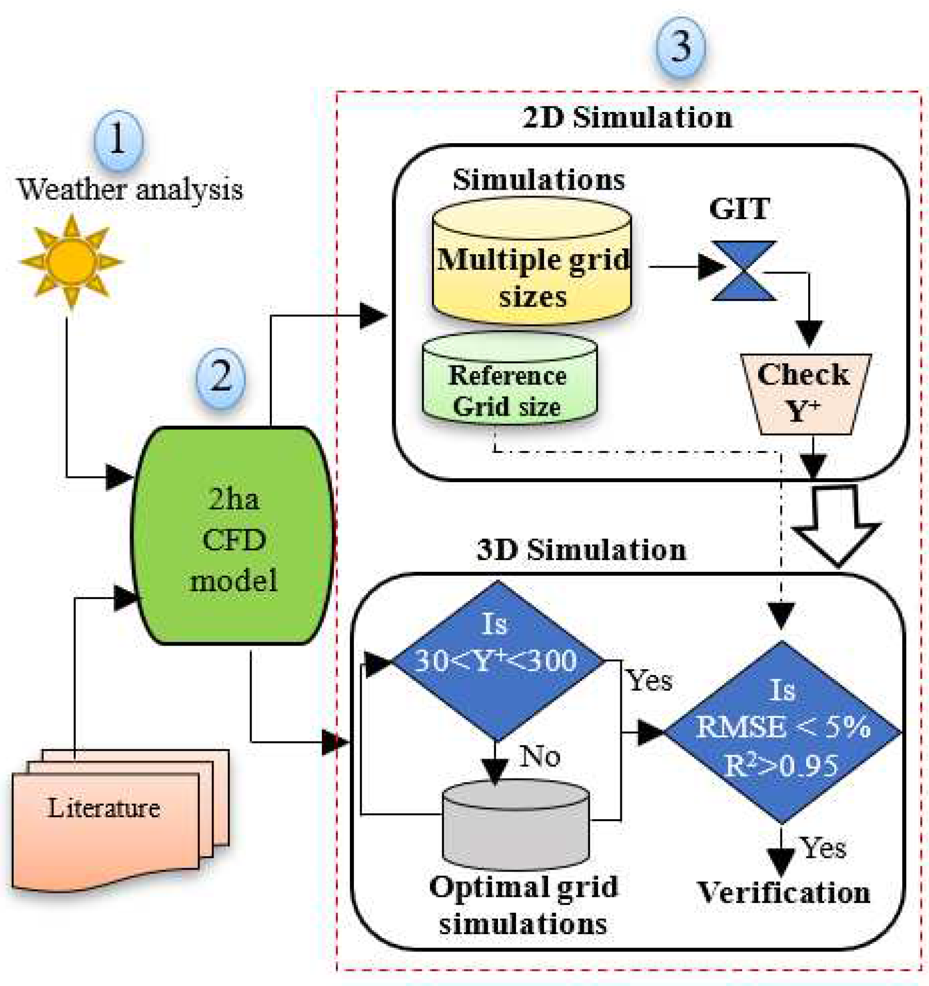
Figure 2. Flow chart of overall research procedure.
Preprints 79290 g002
Figure 5. Overall 3D computational domain, crop canopy domain and greenhouse domain.
Preprints 79290 g005
Figure 6. Model verification study procedure.
Preprints 79290 g006
Figure 7. Schematic illustration of (a) analysis regions and air velocity profile analysis distances from the center, (b) the analysis surfaces and verification data extraction points.
Preprints 79290 g007
Figure 8. Schematic illustration of the vertical heights at which the study parameter distribution was analyzed within the crop canopy.
Preprints 79290 g008
Figure 9. Greenhouse average air velocity for reference simulation (0.2 m) and for larger grid size simulations (0.3 m ~3.0 m) used for GIT.
Preprints 79290 g009
Figure 10. Y+ in 2D model (a) before near wall refinement. Y+ in 3D model (b) after near wall refinement with first layer height of 0.04 m.
Preprints 79290 g010
Figure 11. Air velocity correlation between the reference grid size (0.2m) and the selected optimal grid size (0.8m) at analysis heights 0.7m, 2.2m and 3.5m.
Preprints 79290 g011
Table 1. Wind profile turbulent kinetic energy and Dissipation rate design parameters.
Parameter Value
Karman constant(k) 0.42
Roughness length (Z0) 0.03 m
Empirical constant 0.09
Reference height ( z R ) 10 m
Summer average wind speed 3.08 m·s-1
Frictional velocity (u*) 0.227 m·s-1
Table 2. Ventilation requirement evaluation parameters and values.
Parameter Symbol Value
Volumetric specific heat of air (Wm-3 oC-1) CV 0.3
Correction rate of heated area α 1.2
Solar transmissivity of greenhouse cover τ 0.7
Solar radiation (Wm-2.m-1) s 200,400,600,800
Evapotranspiration coefficient (Tomato) f 0.5
Temperature difference (℃) ∆T 1~7
Overall heat transfer ceff.(Wm2.min-1. oC -1) K 0.08
Greenhouse flow area (m2) Af 19200
Greenhouse cover area(m2) Ac 24,946.3
Greenhouse volume(m3) V 124800
Disclaimer/Publisher’s Note: The statements, opinions and data contained in all publications are solely those of the individual author(s) and contributor(s) and not of MDPI and/or the editor(s). MDPI and/or the editor(s) disclaim responsibility for any injury to people or property resulting from any ideas, methods, instructions or products referred to in the content.
Copyright: This open access article is published under a Creative Commons CC BY 4.0 license, which permit the free download, distribution, and reuse, provided that the author and preprint are cited in any reuse.
Prerpints.org logo

Preprints.org is a free preprint server supported by MDPI in Basel, Switzerland.

Subscribe

© 2024 MDPI (Basel, Switzerland) unless otherwise stated