
Submitted:
13 July 2023
Posted:
14 July 2023
You are already at the latest version
Abstract
For the first time VIS/NIR-SWIR (visible and near infrared – shortwave infrared) nighttime spectra of a satellite mission are analyzed, using the EnMAP (Environmental Mapping and Analysis Program) high-resolution imaging spectrometer. The focus of this article is set on the spectral characteristics. First, the spectral calibration of EnMAP is checked based on sodium emissions of lighting. Here, applying a realized novel general method, shifts of +0.3nm for VIS/NIR and −0.2nm for SWIR are identified with uncertainties analyzed to be in the range of [−0.4nm,+0.2nm] for VIS/NIR and [−1.2nm,+1.0nm] for SWIR. These results emphasize the high accuracy of the spectral calibration of EnMAP and illustrate the feasibility of methods based on nighttime Earth observations for the spectral calibration of future nighttime satellite missions. Second, applying a realized simple general method, the dominant lighting types of Las Vegas, Nevada, USA, and thermal emissions are identified per pixel and the consistency of the outcomes is considered. These results illustrate the feasibility of the precise identification of lighting types and thermal emissions based on nighttime high-resolution imaging spectroscopy satellite products and support the specification of, in particular, spectral characteristics of future nighttime missions.
Keywords:
EnMAP
; imaging spectroscopy
; nighttime remote sensing
; spectral calibration
; lighting types
1. Introduction
Nocturnal optical remote sensing in the visible and near infrared (VIS/NIR) and short-wave infrared (SWIR) of the electromagnetic spectrum is largely challenging both to its daytime counterpart as well as to nighttime remote sensing in the thermal infrared. This is even more prominent when considering spectral-resolved data and ground resolutions of approx. . Even if there is a large gap in terms of the amount and the diversity of available missions and products, there exists a demand for such nighttime products. The interest in such products is growing as evident from the increasing number of applications [10]. These include the monitoring of human settlements and urban dynamics, the estimation of demographic and socio-economic information, light pollution and its influence on ecosystems, human health and astronomical observations, energy consumption and demands, detection of gas flares, active volcanoes and forest fires, natural disaster assessment and the evaluation of political crises and wars [13,14]. Most of these applications are derived from data linked to artificial lights which emit mainly in the VIS/NIR, but also in the SWIR. A stronger focus on optical nighttime remote sensing is, therefore, well-founded. One example from the domain of socio-economics is that the lighting type is a much stronger indicator of economic growth than solely the intensity of light as used in most studies [2]. And as economic growth is indirectly related to greenhouse gas emissions from all sectors [21], observations of artificial light and estimates of energy consumption complement existing missions on trace gasses [15]. Furthermore, many other past, present, and planned missions provide information regarding how greenhouse gas emissions affect the global environment.
1.1. Nighttime remote sensing
Today, one of the best sources of nighttime data is the DNB (Day-Night Band) of the Visible Infrared Imaging Radiometer Suite (VIIRS) of the SNPP, NOAA-20, and NOAA-21 missions. This band has a spatial resolution of m with a daily global coverage since 2011 [20,25]. Besides these panchromatic space-based nighttime images, trichromatic ones come in the form of photographs with a spatial resolution between m and m taken by astronauts aboard the International Space Station (ISS) irregularly since 2003 [18,19]. Some other spaceborne missions also acquired panchromatic or multispectral data during nighttime. However, in the hyperspectral domain, no spaceborne but only a few airborne missions acquired hyperspectral data during nighttime, e.g. the AVIRIS [7] and the SpecTIR system [12].
1.2. EnMAP imaging spectroscopy mission
EnMAP (Environmental Mapping and Analysis Program; www.enmap.org) is a high-resolution imaging spectroscopy remote sensing satellite mission launched at 1st April 2022 and operational since 2nd November 2022 [11,24]. Already at 3rd November 2022, 06:10 UTC, or 2nd November 2022, 23:10 local time, a nighttime Earth observation of Las Vegas, Nevada, USA, was performed. We consider the center of the observation, namely tile 2 as processed at 3rd June 2023, where the complete observation consists of tiles 1 to 3. The observation was performed with a tilt of westwards. For orientation purposes Figure 1 illustrates a colored infrared of an orthorectified EnMAP daytime observation (L1C product) and a color table representation of the integrated VIS/NIR signal of the orthorectified EnMAP nighttime observation (based on L1C data) for the same subset of approx. (width × height) covering in particular the Las Vegas Strip well known for its intense and divers lighting.
In sensor geometry, the standard EnMAP L1B product tile [1,24] provides (width × height or across-track × along-track) pixels each of 30m×30m and 224 continuous bands between 420nm and 2450nm acquired by a prism-based push-broom dual-spectrometer. This is illustrated in Figure 2, where the complete EnMAP tile is depicted; note that this is in sensor geometry and still oriented in South-North direction, because the nighttime observation is performed in the ascending orbit node. Within the figure, the integrated signal for each pixel is shown separately for VIS/NIR (420nm to 900nm) and SWIR (900nm to 2,450nm), where bands in strong atmospheric absorption are not considered and for illustration purposes instead of signal L the value is considered, namely low signals are raised compared to high signals. Hence, for VIS/NIR the signal is similar to VIIRS-DNB (500nm to 900nm), but considering blue light additionally.
Among the pixel with highest signal in VIS/NIR and SWIR is the Luxor Hotel and Casino. As expected for not orthorectified EnMAP tiles, spatial offsets for SWIR to VIS/NIR of approx. pixel in across-track direction and of approx. pixel in along-track direction are clearly visible. Because of the EnMAP instrument, namely the dual-spectrometer, SWIR and VIS/NIR do not observe the same location at the same time, but with a difference of approx. 20 pixel in along-track direction and a minimal difference of approx. 2 pixel in across-track direction due to the shift of the sensors, the tilting of the satellite, and the Earth rotation.
In the following, this article first checks and analyses the spectral calibration and the related uncertainties in Section 2 for the mentioned nighttime EnMAP tile. Second, the identification of the dominant lighting types is presented and analysed in Section 3. The article finishes with a conclusions covering summary and outlook in Section 4.
2. Checks of spectral calibration
In 2000, [4] checked the spectral calibration of AVIRIS based on a nighttime observation of Las Vegas, Nevada, USA. The study focused on a specific and known light source, namely of the MGM Grand Hotel, having strong and narrow emissions at 535nm. Due to the coarser spatial resolution of EnMAP, and as the lighting type of this particular area is anticipated to have changed between 2000 and 2022 (see Section 3.2), we modified the approach using the various lighting types are measured precisely in the laboratory by [8].
Therefore, we consider a similar approach as [4], but account for a set of narrow sodium emissions lines at 819nm and 1,139nm as analysed in Section 2.1 and we consider resulting uncertainties in Section 2.2.
2.1. Methods and Results
Within this study, we consider the spectral features of High-Pressure Sodium (HPS), Metal Halide (MH), and Low-Pressure Sodium (LPS) lamps. The spectra of HPS and MH have strong peaks at 819nm and 1,139nm (typically strongest in VIS/NIR and SWIR). And the spectrum of LPS has a medium peak at 819nm and a low peak at 1,139nm. Furthermore, the signals are higher in VIS/NIR than in SWIR. These spectra were measured by [8] and the sums of the signals normalized to 1 are illustrated in Figure 3. Other lighting types measured by [8] do not have strong and narrow emissions in this region as illustrated in Section 3.2. For VIS/NIR, we even do not expect other strong influences. For SWIR, we do expect some influences based on stronger thermal emissions and resulting from stronger atmospheric absorption effects resulting in higher uncertainties.
We are especially interested in shifts of center wavelengths of the EnMAP bands which is expected to have the major influence on changes of the spectra. To be more precise, we expect constant shifts of the center wavelengths (CW) of the bands in the considered ranges of approx. nm with respect to the peak of the emission, namely all bands are shifted by the same value, the Full Width at Half Maximum (FWHM) and radiometry are expected to be correct, namely as stated in the metadata of the product, and the Spectral Response Function (SRF) is expected to be a Gaussian function [24].
Next, in frame of this study we make assumptions, marked as (A#), and analyse these also in relation to uncertainties in Section 2.2.
First, we consider one of the seven spectra measured by [8] as reference spectrum (A1), namely the HPS spectrum illustrated in Figure 3 (red solid line). As the differences of the spectra are limited in the considered ranges and the EnMAP observation is expected to contain a mixture of these spectra, we do expect minor influences on the check of the spectral calibration, here. Furthermore, it is expected, that the luminous efficacy of the lighting types, namely how well a light source produces visible light given by the ratio of luminous flux to power, is improved for 2022 compared to 2010, but most lighting types are not changed and, in particular, the physical properties of the light emissions and resulting spectra have not changed.
EnMAP observes light emissions either directly (i.e., upwards from the light source to the sensor) or indirectly (i.e., downwards from the light source, reflected by the Earth surface, and upwards to the sensor). In both cases the signal is influenced by the path upwards through the atmosphere. Thus, we consider all light emissions per pixel observed either directly or indirectly via a smooth surface (i.e., constant, positive reflectance) in each of the considered ranges (A2). It is expected that most light emissions are observed directly and furthermore, typical surface reflectances are basically smooth and without narrow absorption features in each of the considered ranges [17]. Therefore, we do expect minor influences on the check of the spectral calibration.
We consider a standard atmosphere (A3), namely an urban mid-latitude summer atmosphere at nadir with a default water vapour of 3,635.9atm-cm [16], because more detailed information are typically absent, e.g. not stated in the metadata of the product. Because the dynamics of the atmosphere are limited in the considered ranges, namely the change of the atmosphere in the EnMAP observation is limited, the differences of the atmospheric transmission between a maximal, a default, and a minimal water vapour is basically constant in each of the considered ranges as illustrated in Figure 4, and also other atmospheric parameters have limited non-constant effects, we do not expect major influences on the check of the spectral calibration, here.
Finally, we consider ranges of bands with respect to the peaks of the emission (A4), namely ranges of approx. nm with respect to 819nm for VIS/NIR and 1,139nm for SWIR. These ranges cover symmetrically the complete spectral range around the lighting emission feature, namely low signals (bands and ), medium signals (bands and ), high signals (bands and ), but no other spectral features.
Figure 5 illustrates the resulting image spectra for shifts of the center wavelengths for EnMAP based on the spectral calibration of nm, nm, and nm (bluish, greenish and yellow lines) with respect to the reference spectrum (red line).
To estimate the shift for an image spectrum, we normalize the sum of the signal of the bands in the considered range to 1, in particular for consistent results of the distance measure. Thereby, the absolute signal intensity is excluded in the shift estimation. For the fitting of the image spectrum to the reference spectrum, the error of the normalized signal is used, where the minimum error represents the best fit. We consider the Euclidean distance as the error of two spectra (A5), namely the standard distance measure [6].
Finally, let us analyse different approaches for selecting an image spectrum to estimate the shift (A6), which is highly relevant for the low signals in nighttime observations. In the next, four cases are investigated: using arbitrary pixel (Arbitrary), using high intensity pixel (Maximum) and sum (or averaging) over all pixel (Sum), and an optimized method based on the results of the first cases.
Arbitrary. In this case we consider an arbitrary image spectrum (light gray lines) of the 1,024,000 image spectra, e.g. the center pixel, and the fitted reference spectrum (light green lines) as illustrated in Figure 6. We obtain shifts of nm for VIS/NIR and nm for SWIR. However, the signals are lower with W/m/sr/nm for VIS/NIR and W/m/sr/nm for SWIR as also discussed in Section 2.2. Therefore, major influences of noise are expected and visible through large errors of for VIS/NIR and for SWIR. Therefore, for this study this approach seems to be not feasible and is thus discarded.
Maximum. In this scenario we consider an image spectrum with a maximal signal with respect to the considered range (dark gray lines) and the fitted reference spectrum (dark green lines) as illustrated in Figure 6. We obtain shifts of nm for VIS/NIR and nm for SWIR. Now, the signals are higher with W/m/sr/nm for VIS/NIR and W/m/sr/nm for SWIR. And the errors are for VIS/NIR, namely smaller as for the center pixel, and for SWIR, namely larger as for the center pixel. Minor influences of noise are expected, but random effects for a single pixel are expected as illustrated, e.g. based on stronger thermal emissions in SWIR, namely outliers have a major influence the results and the approach seems to be feasible in parts.
Sum. Finally, we consider more than a single image spectrum. To be more precise, we consider the sum of the 1,024,000 image spectra (black lines) and the fitted reference spectrum (blue lines) as illustrated in Figure 6. We obtain shifts of nm for VIS/NIR and nm for SWIR. The signals are highest with W/m/sr/nm for VIS/NIR and W/m/sr/nm for SWIR. The errors are for VIS/NIR and for SWIR. Because most of the incorporated image spectra are of lower signal, raising of the signals and hiding of the reference spectra are expected and visible through close to constant summed image spectra for VIS/NIR and SWIR and the approach seems to be feasible in parts.
Optimum. Based on these results, in particular of the scenarios Maximum and Sum, we consider the image spectra ordered from high signals to low signals with respect to the considered range, namely a mixture of Maximum and Sum. To be more precise, we consider the spectrum resulting as sum of the image spectra of the highest signals for . We already analyzed and in the paragraphs Maximum and Sum. Let be the correspondingly observed error and let nm be the observed shift. We expect larger changes in the error (and shift), if i is small, because of the larger influence of random effects for single pixel, as illustrated in Figure 7 (top). And we expect smaller changes in the error (and shift), if i is large, because of the smaller influence of an extra pixel, which has at most the same signal influencing the sum as the prior considered pixel, as illustrated in Figure 7 (bottom). We intent to identify the spectrum with minimal error , but for i large enough to be not strongly affected by outliers. Future research may consider outliers and radiometric uncertainties in a more sophisticated way.
To be more precise, for a given relative deviation in the error , let , namely the first index such that for all consecutive indices of at least the relative deviation in the error is at most e, and let , namely the first index of at least with a minimal error. We consider (A5), namely the relative deviation in the error shall be at most 1%.
Finally, we obtain nm for VIS/NIR and nm for SWIR, where , , and for VIS/NIR as well as , , and for SWIR. Figure 6 illustrates the spectra of the optimally summed image spectra (yellow lines) and the fitted reference spectra (red lines).
2.2. Sensitivities and Influences of Assumptions
In the following, we analyze the sensitivity of the method and the influences of the assumptions made in Chapter 2.1, resulting in the expected uncertainty range of this approach.
Sensitivity to noise. For the analysis of sensitivity to noise of the estimated shifts, we expect that the spectra are predominantly affected by signal independent Gaussian noise and only to a small degree affected by signal dependent shot noise [22], because of the low signals, e.g. by comparing the optimally summed image spectra and the fitted reference spectra as illustrated in Figure 6. Furthermore, we expect that the noise is equally distributed to all bands, because, e.g. by examining half of the image spectra with the lower signals in the considered range, we obtain
- for VIS/NIR signals, averaged for each band, in the range of W/m/sr/nm with standard deviations in the range of and
- for SWIR signals, averaged for each band, in the range of W/m/sr/nm with standard deviations in the range of ,
namely, basically constant signals, averaged for each band, with constant standard deviations. Furthermore, for these image spectra, we obtain
- for VIS/NIR a signal, averaged for all bands, of W/m/sr/nm with a standard deviation of , namely an expected relative deviation of the signal of , and
- for SWIR a signal, averaged for all bands, of W/m/sr/nm and a standard deviation of , namely an expected relative deviation of the signal of .
Based on these estimates for the given case, the noise contribution is larger in VIS/NIR than in the SWIR.
For estimating the sensitivity, we add noise to the reference spectrum and change its shift to achieve an observed error and shift. In particular, if some ratio of the signal of the normalized, not noisy, shifted by nm, reference spectrum with is equally added to each of the b considered bands as noise, namely the noisy, shifted by nm, reference spectrum is considered, we obtain an observed error and shift.
To be more precise, we consider the mapping . This mapping f is not necessarily bijective, in particular not unambiguous, because different combinations of r and c may result in the same observed error and shift , namely f is not injective as , or no combinations of r and c may result in some observed error and shift , namely f is not surjective as . The mapping f is illustrated in Figure 8.
Consequently, the influence of noise for the observed errors and shifts in Section 2.1 is as follows. For the VIS/NIR, the estimates have minimal ambiguities and just a minor change in the spectral shift of nm. For the SWIR, ambiguities increase to and a related major change in the shift of is observed.
Because of the observations on noise, namely accounting for the expected relative deviations of the signals, averaged for all bands, of for VIS/NIR and for SWIR, we consider ratios for VIS/NIR and for SWIR. In other words, we consider some more added noise to the reference spectrum. Hence, at most all for , namely is not considered as outlier, and where for and any c, are shifts not violating the expected deviations of the observed errors. We obtain ranges for VIS/NIR and for SWIR and by considering any c, where for , and any , we obtain results on uncertainties based on sensitivity as stated in Table 1. We remark, at least for the considered ranges, the values of and r are strongly correlated by a constant positive factor. Because, e.g., for VIS/NIR and for SWIR, Figure 7 (lines 1 and 2) indicates these ranges of D and Figure 8 indicates the resulting differences, namely uncertainties. We remark, nm is always contained in the ranges, here, because for the noisy and not noisy spectra equal.
A1—influence of lighting types. Let us consider assumption A1 and each of the seven spectra measured by [8] as reference spectrum (HPS, MH, LPS). We obtain shifts of:
| reference | |||||||
| HPS 1 | HPS 2 | HPS 3 | MH 1 | MH 2 | MH 3 | LPS | |
| VIS/NIR | nm | nm | nm | nm | nm | nm | nm |
| SWIR | nm | nm | nm | nm | nm | nm | nm |
Because of lower signals for LPS in VIS/NIR and SWIR, and as mixtures of such spectra are expected, we do not account for (and to avoid drifts both) the minimum shifts, marked by (1), and maximum shifts, marked by (2). As expected, the differences in the shifts are marginal and we obtain results on the uncertainties based on A1 as stated in Table 1. We remark, that the average shifts are nm for VIS/NIR and nm for SWIR and, in particular for VIS/NIR, these shifts are close to the shifts for the reference spectrum.
A2—influence of surface types and upward vs. downward illuminations. Let us consider assumption A2 and a smooth surface reflectance, absorption depths of low (00.1%), medium (01.0%), and high (10.0%) and absorption widths of low (001nm), medium (010nm), and high (100nm) applied to the constant, positive surface reflectance. In other words, if a signal is a combination of, e.g., 90% directly observed light emission and 10% indirectly observed light emission via a surface with a positive reflectance, and now a high absorption depth of 10.0% is applied to the surface, namely the surface reflectance is changed by a factor of 90.0%, then a signal of results. We remark, that the result is the same as for, e.g., 0% directly and 100% indirectly observed light emission and applying a medium absorption depth of 01.0%. To be more precise, we model absorption of at a specific wavelength of nm by a linearly descending absorption to the constant, positive surface reflectance by a factor of at nm to for increasing distances to nm, where the Full Width at Half Maximum is given by . Considering all nm, we obtain shifts of:
| VIS/NIR | low depth (00.1%) | medium depth (01.0%) | high depth (10.0%) |
| low width (001nm) | |||
| medium width (010nm) | |||
| high width (100nm) |
| SWIR | low depth (00.1%) | medium depth (01.0%) | high depth (10.0%) |
| low width (001nm) | |||
| medium width (010nm) | |||
| high width (100nm) |
As expected, the extends of the ranges increase by increasing the absorption depths and are larger for medium widths, because for low widths the influence to a single band is limited and for large widths the influence to all bands is similar. We account for the minimum and maximum shifts for all considered combinations of and and we obtain results on the uncertainties based on A2 as stated in Table 1.
A3—influence of atmospheres. Let us consider assumption A3 and next to the default atmosphere, atmospheres with a maximal (but not cloudy) and a minimal water vapour of 6651.1atm-cm and 1817.9atm-cm, that is half of the default water vapour, as illustrated in Figure 4. Because the water vapour has the highest influence on the atmospheric absorption, we do not consider changes of the other parameters. We obtain shifts of nm and nm for VIS/NIR, and nm and nm for SWIR. In particular for VIS/NIR, the shifts are close to the ones for the default atmosphere, because the dynamics of the atmosphere are limited in this wavelength range. And we obtain results on the uncertainties based on A3 as stated in Table 1. We remark, if we do not account for the atmosphere at all, shifts of nm for VIS/NIR and nm for SWIR result, that are as expected close to the shifts considering the default atmosphere.
A4—influence of range of bands around the lighting emission peaks. Let us consider assumption A4 and next to the default range of bands, bands and bands around the lighting emission peaks, namely 819nm for VIS/NIR and 1,139nm for SWIR. We obtain shifts of nm and nm for VIS/NIR and nm and nm for SWIR. Again, in particular for VIS/NIR, these are close to the shifts for the default range of bands. And we obtain results on the uncertainties based on A4 as stated in Table 1. This assumption is already incorporated by the considerations of sensitivity, namely changes of the considered bands will result in corresponding changes in the sensitivity, and therefore, not relevant for uncertainty estimations. However, the results illustrate the robustness of the considered method.
A5—influence of distance metrics. Let us consider assumption A5 and for normalized image spectra and reference spectra next to the default Euclidean distance , the Manhattan distance and the distance . We obtain shifts of nm and nm for VIS/NIR and nm and nm for SWIR, namely, in particular for VIS/NIR, close to the shifts for the default distance measure. And we obtain results on the uncertainties based on A5 as stated in Table 1. This assumption is already incorporated by the considerations of sensitivity, namely changes of the considered distance measure will result in corresponding changes in the sensitivity, and therefore, not relevant for uncertainty estimations, here. However, the results illustrate the robustness of the considered method.
A6—influence of image spectra selections. Let us consider assumption A6 and next to the default relative deviation in the error of , and —as well as , , and for later investigations—, namely lower and higher values as the default. We obtain shifts of:
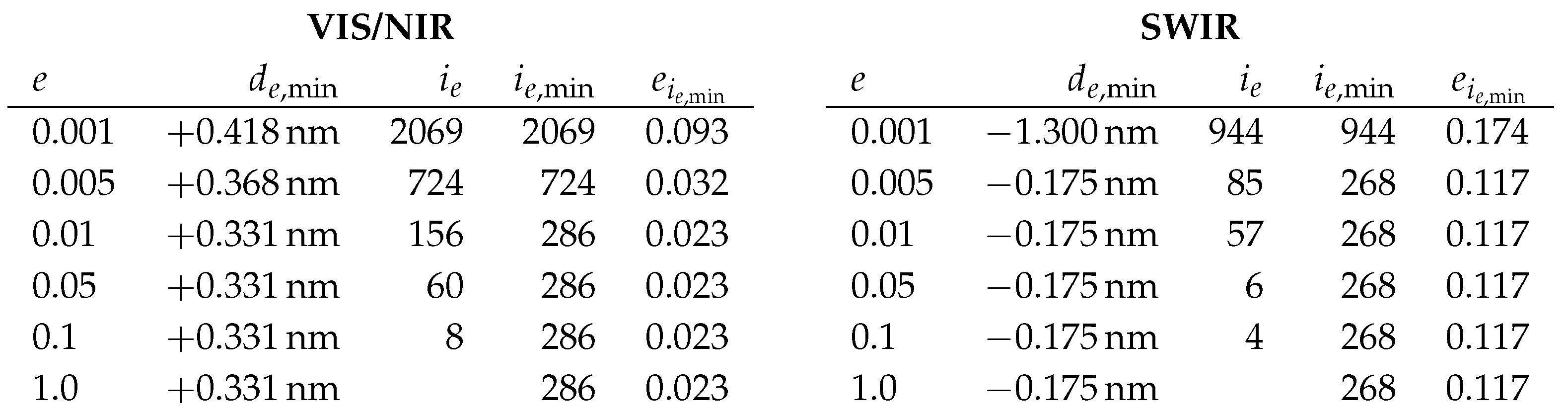
Because for VIS/NIR, this may be seen as some indicator, that is a too conservative value, here, but nevertheless the shift for is close to the one for and for SWIR . Furthermore, for we obtain for VIS/NIR and SWIR. And we obtain results on uncertainties based on A6 as stated in Table 1. Because all these observed errors and shifts are already incorporated by the considerations of sensitivity, this assumption is not relevant for uncertainty estimations, here. We remark, if we consider and , namely we do not consider e at all, but any optimum, we obtain the same shifts as for . Furthermore, because for VIS/NIR and SWIR, this may be seen as strong indicator, that is a too conservative value, here.
Summary of A1 to A6. Assuming to the worst that all these estimated uncertainties typeset bold in Table 1 are correlated, namely the ranges need to be added, we obtain total uncertainties as stated in Table 1, namely expected shifts of nm in the range for VIS/NIR and nm in the range for SWIR. These values—even the estimated shifts and not considering the estimated uncertainties—are well within the accuracy of nm for the spectral calibration based on laboratory calibrations and dedicated satellite equipment [24]. We remark, assuming shifts of nm for VIS/NIR and nm for SWIR lead to symmetric uncertainties of nm for VIS/NIR and for SWIR.
In addition to the investigation of other spectral features of light emissions, future research may consider atmospheric absorption features such as the Oxygen A band absorption at 760nm or the CO absorption at 2,060 for homogeneous light or thermal emissions in that range.
Figure 9 illustrates for the complete EnMAP tile the integrated signals for each pixel accounting for the bands in the considered range, where for illustration purposes instead of signal L the value is considered. We remark, for VIS/NIR, marginal systematic striping effects in along-track direction and for SWIR, marginal systematic higher signals at the borders compared to the center in across-track direction are visible.
Spectral Along-Track Stability. Another aspect is to check the spectral stability over short time intervals, i.e. in along-track direction. If we split the EnMAP tile into the first half and second half in along-track direction, we observe that pixel with high signals are located in both halves and we obtain shifts of nm (with error ) and nm (with error ) for VIS/NIR and nm (with error ) and nm (with error ) for SWIR. All these estimated shifts are close to the estimated shifts for the complete EnMAP tile and, in particular, well within the estimated uncertainties. Thus for this given scene the described approach allows for the estimation of short time stability, which is given for EnMAP.
Spectral Across-Track Characteristics. As hyperspectral push-broom sensors often exhibit a slight change in center wavelengths in across-track direction (often denoted as spectral smile), this sensor property is also assessed with this method. For the EO tile, we observe that pixel with high signals are located, in particular, between approx. pixel 570 and 630 in across-track direction or of the sensor. To be more precise, for the average—weighted based on the considered signals of the considered pixel—sensor pixel is for VIS/NIR and for SWIR. For these sensor pixel shifts of nm for VIS/NIR and nm for SWIR are expected according to the spectral calibration based on laboratory characterization. Therefore, accounting for the shifts of these sensor pixel, too, we assume shifts of nm for VIS/NIR and nm for SWIR.
To analyze the spectral smile, we separate the 1,000 valid sensor pixel per band to 4 parts of 250 pixel each. We consider the two parts with lowest fitting error. And we obtain shifts of nm (with error ) and nm (with error ) for the 3rd and 4th part of VIS/NIR (all other parts have errors of at least ) and nm (with error ) and nm (with error ) for the 3rd and 4th part of SWIR (all other parts have errors of at least ). Figure 10 illustrate these results. All these results are well within the estimated uncertainties.
For VIS/NIR, the estimated smile is highly consistent, being close to the estimate using a across-track constant fitting, and showing the same across-track slope as the smile based on laboratory calibrations. For SWIR, where the uncertainties are estimated to be much larger as for VIS/NIR, the estimated shifts are decreasing with increasing across-track pixel as for the spectral calibration based on laboratory calibrations, but the magnitudes of changes are not consistent.
3. Identifications of lighting types
In 2011, [12] identified the lighting types of parts of Las Vegas, Nevada, USA, based on a nighttime observations of a SpecTIR system. The binary encoder approach of [12] was used to identify the dominant lighting type for a pixel, considers the emissions of different, known lighting types measured precisely in the laboratory by [8] in 2010. Furthermore, already in 2005, [5] estimated the thermal emission considering Planck’s law based on a daytime observation of AVIRIS. The best fit approach of [5] to optimize the retrieval of temperature and corresponding areal fractions for a pixel, considers a solar reflected and a thermal emitted part. Based on the analysis in Section 2, we focus on a combined approach as [12] and [5], and consider the full shape of the spectra and lighting types based on laboratory measurements and Planck’s law, here, as analysed in Section 3.1 and we discuss the results in Section 3.2.
3.1. Methods
We consider the full spectra of three High-Pressure Sodium (HPS), three Metal Halide (MH), and one Low-Pressure Sodium (LPS) lamps as already considered in Section 2, as well as three Incandescent (INC), three Liquid Fuel (LIQ), three Pressured Fuel (PRES), one Mercury Vapor (MV), two Quartz Halogen (QH), three Fluorescent (FL), and nine Light Emitting Diodes (LED). For LEDs, these include two Cold White (CW), two Natural White (NW), one Blue, one Green, one Red, and two Yellow light emission spectra. These spectra were measured by [8]. Furthermore, we consider the full spectra of thermal emissions for temperatures based on Planck’s law and covering temperatures of different types for fires, e.g., associated with biomass burning, typically 900K to 1,200K, and gas flaring, typically 1,400K to 2,400K, [9].
For VIS/NIR, we consider all bands between nm and nm only, because we typically do not expect high signals for wavelengths between nm to nm based on the typical lighting types. For SWIR, we consider all bands, where the atmospheric transmissions are for the default atmosphere and the difference between the atmospheric transmissions for the default and maximum atmosphere is for the atmospheres already investigated in Section 2. To be more precise, because we do not consider the ranges nm to nm, nm to nm, and nm to nm, we avoid the influences of strong atmospheric absorption regions and related uncertainties.
We consider a constant, positive surface reflectance, a standard atmosphere, and the Euclidean distance as error metric as in Section 2. To identify the dominant lighting type for an image spectrum, we optimize the scale for each of the considered reference spectra to fit to the image spectrum and consider the lighting type of the reference spectrum with the minimal error as dominant.
Because of the observations on noise in Section 2 and to handle noise accordingly, we consider image spectra with signals by a factor of at least 2 larger than the median. To account for the errors in the identification, we consider all image spectra, where the error between the image spectrum and the best fitting reference spectrum is less than and (default).
Therefore this straightforward spectral identification approach does not aim for separating mixtures of multiple light sources within a pixel, nor aims at the retrieval of surface reflectance properties. Nevertheless, it is well suited to demonstrate the identification and subsequent mapping of nighttime spectra in the VIS/NIR and SWIR ranges based on spectral resolved emission features, which are globally valid for all similar lighting sources.
3.2. Results
Out of the in total 1,024,000 pixel, the method identifies the dominant lighting types for 2,006 and 8,819 pixel for VIS/NIR and for 448 and 451 pixel for SWIR for errors less than and (default) as illustrated in Figure 11, where we obtain the same results for any error larger than . The identification of the dominant lighting types and temperatures are stated in Table 2 and Table 3. For LPS, FL, and LED we do not expect the identification in SWIR and for temperatures we do not expect the identification in VIS/NIR, because of the low signals.
As the spectra of INC, LIQ, and PRES are similar to spectra of temperatures of approx. 1,300K, 1,900K, and 2,300K, we separate the estimation of temperatures once by separating the identified INC/LIQ/PRES, and once by not separating. And we do expect that HPS and MH are less well identified in SWIR than in VIS/NIR, because of the lower signals. If we consider the consistency of identifications between VIS/NIR and SWIR, we have to account for the spatial offset of pixel from SWIR to VIS/NIR as mentioned in Section 1. The correctness of the next observations is visually checked based on nighttime photos of Las Vegas, Nevada, USA, and based on comparisons of the observed and reference spectrum, too.
HPS. We consider the Eiffel Tower of Paris Las Vegas Hotel and Casino contained in pixel 589,551 for VIS/NIR, where the same lighting type is identified for the four neighboring pixel, and in pixel 591,531 for SWIR as illustrated in Figure 12 (line 1). The identified lighting type is consistent with the results by [12].
MH. We consider the Trump International Hotel Las Vegas contained in pixel 582,611 for VIS/NIR, where same lighting type is identified for the four neighboring pixel, and in pixel 584,591 for SWIR as illustrated in Figure 12 (line 2). The shapes of the areas of the identified lighting type is consistent for VIS/NIR and SWIR.
FL. We consider the Venetian Resort Las Vegas contained in pixel 574,588 for VIS/NIR as illustrated in Figure 12 (line 3, left), where low signal is identified in SWIR as expected.
Low temperature of approx. 900K. We consider pixel 207,528 for SWIR and thereby, an area located outside of the Las Vegas Strip, as illustrated in Figure 12 (line 3, right). The temperature is consistent with a bonfire and for neighboring pixel similar temperatures are estimated. To be more precise, in across-track direction the same temperatures are estimated and in along-track direction a gradient from 1,100K (pixel 206,528) to 900K and from 900K to 500K (pixel 208,528) is estimated and illustrates the temperature differences of the anticipated bonfire. The absorption because of CO emissions, in particular between 2,000nm and 2,070nm, is visible in the observed and reference spectrum.
LPS and high temperature of approx. 2,300K. We consider the Bellagio Resort and Casino contained in pixel 589,562 for VIS/NIR and in pixel 591,542 for SWIR as illustrated in Figure 12 (line 4). For VIS/NIR, LPS is identified, where a low signal for SWIR is expected, but for SWIR, a PRES or similar a high temperature of approx. 2,300K is estimated. Therefore, we assume two different dominant lighting types in this case. Furthermore, in SWIR a medium, and in VIS/NIR a low emission of MH lighting is visible. As the spatial offset of SWIR and VIS/NIR is not sub-pixel accurate, likely neighboring pixel are identified as MH.
LED CW and NW. We consider the Caesar Palace Las Vegas Hotel and Casino containing a LED CW, namely with the blue peak higher than the green peak, in pixel 597,584 for VIS/NIR as illustrated in Figure 13 (line 1, left)—and also in the neighboring pixel 597,585— and a LED NW, namely the green peak higher than the blue peak, in pixel 597,582 for VIS/NIR as illustrated in Figure 13 (line 1, right)—and also in the neighboring pixel 598,581.
LED Blue. We consider the Aria Resort and Casino contained in pixel 608,534 for VIS/NIR as illustrated in Figure 13 (line 2, left).
LED Green. We consider the MGM Grand Hotel contained in pixel 597,514 for VIS/NIR as illustrated in Figure 13 (line 2, right). In the study by [4], the modified MH illumination of the MGM Grand Hotel emitting especially green light was used to check the spectral calibration of AVIRIS, where a peak of emissions at 535nm was estimated (see Section 2, too). We estimate a peak of emission at 517nm for the EnMAP tile, a low signal in SWIR, and an uncertainty in the spectral calibration of less than 1nm. Therefore, a change in the lighting type is anticipated between 2010 and 2022, here.
LED Red. We consider the Las Vegas Hilton at Resorts World contained in pixel 560,629 for VIS/NIR as illustrated Figure 13 (line 3, left).
LED Yellow. We consider the Wynn Las Vegas and Encore Resort contained in pixel 566,593 for VIS/NIR as illustrated Figure 13 (line 3, right).
In addition to the investigated identification of the dominant lighting types for higher signals, future research may consider also the identification of lower signal levels as well as the separation of mixed illumination sources. Furthermore, the usage of the combined spectrum instead of VIS/NIR and SWIR separately may be considered.
4. Conclusions
The article performed the first analysis of nighttime light spectra observed by a satellite, more precisely based on one of the first nighttime observations by the high-resolution imaging spectroscopy remote sensing satellite mission EnMAP. The Earth observation covered Las Vegas, Nevada, USA, in the VIS/NIR and SWIR spectral range.
A novel general method was realized to check the spectral calibration of EnMAP in VIS/NIR and SWIR based on sodium emissions of lighting. We identified shifts of nm for VIS/NIR and nm for SWIR compared to the spectral calibration based on laboratory calibrations and the dedicated satellite equipment. Accounting for the sensitivity of the method and the incorporated assumptions, uncertainties were analyzed to be in the range of for VIS/NIR and for SWIR. These results emphasize the high accuracy of the spectral calibration of EnMAP and illustrate the feasibility of methods based on nighttime Earth observations for the spectral calibration of future nighttime satellite missions.
Furthermore, a simple generally valid method was realized to identify per pixel the dominant lighting types based on VIS/NIR and SWIR spectral signatures, also including the thermal emissions also detectable in the SWIR. For the considered targets, the identification results were highly consistent in the VIS/NIR and SWIR ranges.
These results illustrate the feasibility of the precise identification of lighting types and thermal emissions based on nighttime imaging spectroscopy remote sensing satellite products and support the specification of, in particular, spectral characteristics of future nighttime observations [3,23].
Future research may consider more nighttime Earth observations of Las Vegas, Nevada, USA, to further examine the robustness of the methods and changes in urban dynamics over time, but also of other globally distributed human settlements as well as specific sites like gas flares, active volcanoes, and forest fires.
Author Contributions
Conceptualization, M.B. and T.S.; Methodology, M.B. and T.S.; Software, T.S.; Validation, M.B.; Formal Analysis, M.B. and T.S.; Writing — Original Draft Preparation, T.S.; Writing — Review & Editing, M.B.; Visualization, M.B. and T.S.; Supervision, T.S. All authors have read and agreed to the published version of the manuscript.
Funding
This research received no external funding.
Acknowledgments
The authors thank the EnMAP team for providing EnMAP products and in particular, Maximilian Langheinrich for providing the atmospheric transmissions and David Marshall for providing the details on the spectral calibration based on laboratory calibrations and dedicated satellite equipment.
Conflicts of Interest
The authors declare no conflict of interest.
References
- Bachmann, M.; Alonso, K.; Carmona, E.; Gerasch, B.; Habermeyer, M.; Holzwarth, S.; Krawczyk, H.; Langheinrich, M.; Marshall, D.; Pato, M.; Pinnel, N.; de los Reyes, R.; Schneider, M.; Schwind, P.; Storch, T. Analysis-Ready Data from Hyperspectral Sensors—The Design of the EnMAP CARD4L-SR Data Product. Remote Sensing 2023, 4536(1), 1–19. [Google Scholar]
- Bennett, M.M.; Smith, L.C. Advances in using multitemporal night-time lights satellite imagery to detect, estimate, and monitor socioeconomic dynamics. Remote Sensing of Environment 2017, 192, 176–197. [Google Scholar]
- Barentine, J.C.; Walczak, K.; Gyuk, G.; Tarr, C.; Longcore, T. A Case for a New Satellite Mission for Remote Sensing of Night Lights. Remote Sensing 2021, 13(12), 2294. [Google Scholar]
- Chrien, T.G.; Green, R. Using Nighttime Lights to Validate the Spectral Calibration of Imaging Spectrometers. Physics 2000. [Google Scholar]
- Clark, R.N.; et al. Environmental mapping of the world trade center area with imaging spectroscopy after the September 11, 2001 attack: The Airborne Visible/InfraRed Imaging Spectrometer mapping. ACS Publications 2005, 66–83. [Google Scholar]
- Deborah, H.; Richard, N.; Hardeberg, J.Y. A comprehensive evaluation of spectral distance functions and metrics for hyperspectral image processing. IEEE Journal of Selected Topics in Applied Earth Observations and Remote Sensing 2015, 8(6), 3224–3234. [Google Scholar]
- Elvidge, C.D.; Green, R. High- and low-altitude AVIRIS observations of nocturnal lighting. Environmental Science 2005. [Google Scholar]
- Elvidge, C.D.; D.M. Keith; Tuttle, B.T.; Baugh, K.E. Spectral identification of lighting type and character. Sensors 2010, 10(4), 3961–3988.
- Elvidge, C.D.; Zhizhin, M.; Hsu, F.-C.; Baugh, K.E. VIIRS Nightfire: Satellite Pyrometry at Night. Remote Sensing 2013, 5(9), 4423–4449. [Google Scholar] [CrossRef]
- Ghosh, T.; Hsu, F.C. Advances in Remote Sensing with Nighttime Lights. Remote Sensing 2019, Special Issue.
- Guanter, L.; Kaufmann, H.; Segl, K.; Foerster, S.; Rogass, C.; Chabrillat, S.; Küster, T.; Hollstein, A.; Rossner, G.; Chlebek, C.; Straif, C.; Fischer, S.; Schrader, S.; Storch, T.; Heiden, U.; Müller, A.; Bachmann, M.; Mühle, H.; Müller, R.; Habermeyer, M.; Ohndorf, A.; Hill, J.; Buddenbaum, H.; Hostert, P.; van der Linden, S.; Leitao, P.J.; Rabe, A.; Doerffer, R.; Krasemann, H.; Xi, H.; Mauser, W.; Hank, T.; Locherer, M.; Rast, M.; Staenz, K.; Sang, B. The EnMAP spaceborne imaging spectroscopy mission for earth observation. Remote Sensing 1015, 7(7), 8830–8857. [Google Scholar]
- Kruse, F.A., Elvidge, C.D. Identifying and mapping night lights using imaging spectrometry. In Proc. IEEE Aerospace Conference, 2011, USA.
- Kyba, C.C.M.; Pritchard, S.B.; Ekirch, A.R.; Eldridge, A.; Jechow, A.; Preiser, C.; Kunz, D.; Henckel, D.; Hölker, F.; Barentine, J.; Berge, J.; Meier, J.; Gwiazdzinski, L.; Spitschan, M.; Milan, M.; Bach, S.; Schroer, S.; Straw, W. Night Matters—Why the Interdisciplinary Field of "Night Studies" Is Needed. J 2020, 3(1), 1–6. [Google Scholar]
- Levin, N.; Kyba, C.C.M.; Zhang, Q.; Sánchez de Miguel, A.; Román, M.O.; Li, X.; Portnov, B.A.; Molthan, A.L.; Jechow, A.; Miller, S.D.; Wang, Z.; Shrestha, R.M.; Elvidge, C.D. Remote sensing of night lights: A review and an outlook for the future. Remote Sensing of Environment 2020, 237, 111443. [Google Scholar]
- Martin, R.V. Satellite remote sensing of surface air quality. Atmospheric Environment 2008, 42(34), 7823–7843. [Google Scholar]
- Mayer, B.; Kylling, A. The libRadtran software package for radiative transfer calculations-description and examples of use. Atmospheric Chemistry and Physics 2005, 5(7), 1855–1877. [Google Scholar]
- de Meester, J.; Storch, T. Optimized Performance Parameters for Nighttime Multispectral Satellite Imagery to Analyze Lightings in Urban Areas. Sensors 2020, 20, 3313. [Google Scholar]
- de Miguel, A.S.; Kyba, C.C.M.; Aubé, M.; Zamorano, J.; Cardiel, N.; Tapia, C.; Bennie, J.; Gaston, K.J. Colour remote sensing of the impact of artificial light at night (I): The potential of the International Space Station and other DSLR-based platforms. Remote Sensing of Environment 2019, 224, 92–103. [Google Scholar]
- de Miguel, A.S.; Zamorano, J.; Aubé, M.; Bennie, J.; Gallego, J.; Ocaña, F.; Pettit, D.R.; Steffanov, W.L.; Gaston, K.J. Colour remote sensing of the impact of artificial light at night (II): Calibration of DSLR-based images from the International Space Station. Remote Sensing of Environment 2021, 264, 112611. [Google Scholar]
- Miller, S.D.; Straka, W.; Mills, S.P.; Elvidge, C.D.; Lee, T.F.; Solbrig, J.; Walther, A.; Heidinger, A.K.; Weiss, S.C. Illuminating the capabilities of the Suomi National Polar-orbiting Partnership (NPP) Visible Infrared Imaging Radiometer Suite (VIIRS) Day/Night Band. Remote Sensing 2013, 5(12), 6717–6766. [Google Scholar]
- Ou, J.; Liu, X.; Li, X.; Li, M.; Li, W. Evaluation of NPP-VIIRS nighttime light data for mapping global fossil fuel combustion CO2 emissions: a comparison with DMSP-OLS nighttime light data. PloS one 2015, 10(9), e0138310. [Google Scholar]
- Rasti, B.; Scheunders, P.; Ghamisi, P.; Licciardi, G.; Chanussot, J. Noise Reduction in Hyperspectral Imagery: Overview and Application. Remote Sensing 2018, 10(3), 482. [Google Scholar]
- Storch, T.; Aubé, M.; Bara, S.; Falchi, F.; Kuffer, M.; Kyba, C.; Levin, N.; Oszoz, A.; Román, M.O.; de Miguel, A.S.; Schrott, L.; Münzenmayer, R.; Riel, S.; Gaston, K.J. N8—Global Environmental Effects of Artificial Nighttime Lighting. ESA Living Planet Symposium 2022, Germany. [Google Scholar]
- Storch, T.; Honold, H.-P.; Chabrillat, S., Habermeyer, M.; Tucher, P.; Brell, M.; Ohndorf, A., Wirth, K.; Betz, M.; Kuchler, M.; Mühle, H.; Carmona, E.; Baur, S.; Mücke, M.; Löw, S.; Schulze, D.; Zimmermann, S.; Lenzen, C.; Wiesner, S.; Aida, S.; Kahle, R.; Willburger, P.; Hartung, S.; Dietrich, D.; Pleasia, N.; Tegler, M.; Schork, K.; Alonso, K.; Marshall, D.; Gerasch, B.; Schwind, P.; Pato, M.; Schneider, M.; de los Reyes, R.; Langheinrich, M., Wenzel, J.; Bachmann, M.; Holzwarth, S.; Pinnel, N.; Guanter, L.; Segl, K.; Scheffler, D.; Foerster, S.; Bohn, N.; Bracher, A.; Soppa, M.A.; Gascon, F.; Green, R.; Kokaly, R.; Moreno, J.; Ong, C.; Sornig, M.;Wernitz, R.; Bagschik, K.; Reintsema, D.; La Porta, L.; Schickling, A.; Fischer, S. The EnMAP imaging spectroscopy mission towards operations. Remote Sensing of Environment, 2021, 263, 112557.
- Wang, Z.; Román, M.O.; Kalb, V.L., Miller, S.D.; Zhang, J.; Shrestha, R.M. Quantifying uncertainties in nighttime light retrievals from Suomi-NPP and NOAA-20 VIIRS Day/Night Band data. Remote Sensing of Environment, 2021 263, 112557.
Figure 1.
ColorInfraRed (CIR) composite of an orthorectified EnMAP daytime observation (left) and a color table presentation of the integrated VIS/NIR signal of the orthorectified EnMAP nighttime observation (right). EnMAP data © DLR 2022. All rights reserved.
Figure 1.
ColorInfraRed (CIR) composite of an orthorectified EnMAP daytime observation (left) and a color table presentation of the integrated VIS/NIR signal of the orthorectified EnMAP nighttime observation (right). EnMAP data © DLR 2022. All rights reserved.
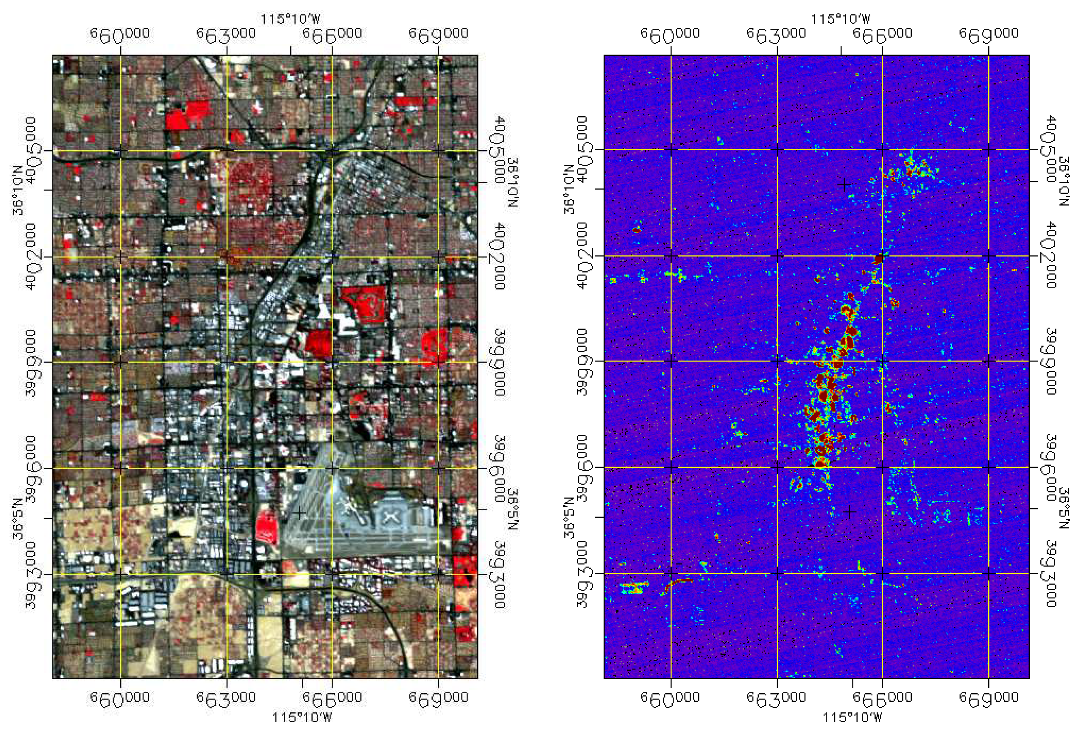
Figure 2.
Integrated signals of VIS/NIR (left) and SWIR (right) of the EnMAP nighttime observation in sensor geometry; the area covered is approx. . EnMAP data © DLR 2022. All rights reserved.
Figure 2.
Integrated signals of VIS/NIR (left) and SWIR (right) of the EnMAP nighttime observation in sensor geometry; the area covered is approx. . EnMAP data © DLR 2022. All rights reserved.
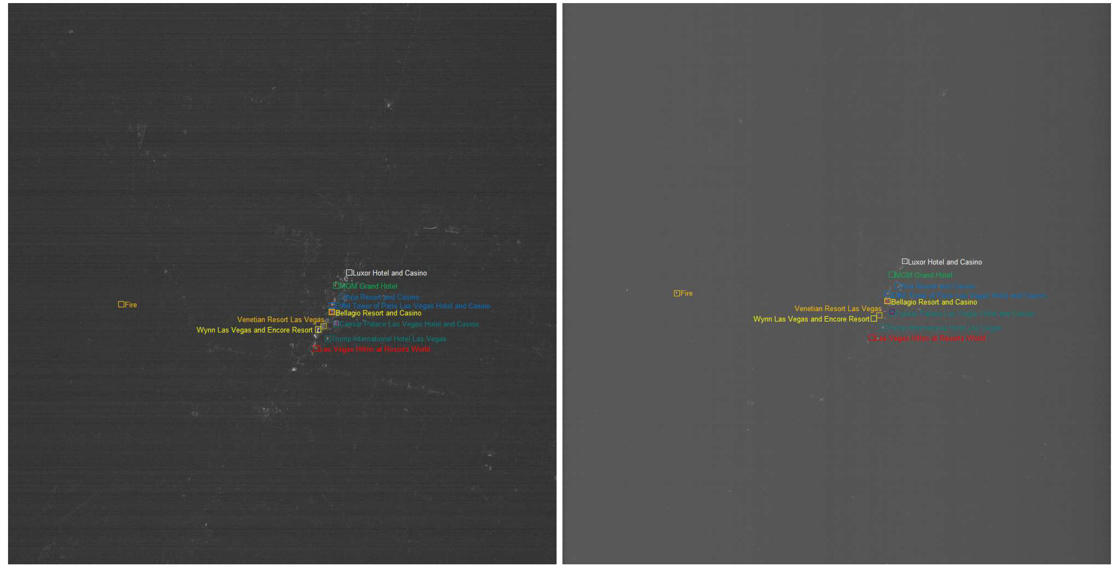
Figure 3.
Reference HPS spectrum (red solid line), other HPS spectra (red dashed lines), MH spectra (orange lines) and the LPS spectrum (yellow line) at 1nm resolution for VIS/NIR (top) and SWIR (bottom) in the considered ranges.
Figure 3.
Reference HPS spectrum (red solid line), other HPS spectra (red dashed lines), MH spectra (orange lines) and the LPS spectrum (yellow line) at 1nm resolution for VIS/NIR (top) and SWIR (bottom) in the considered ranges.
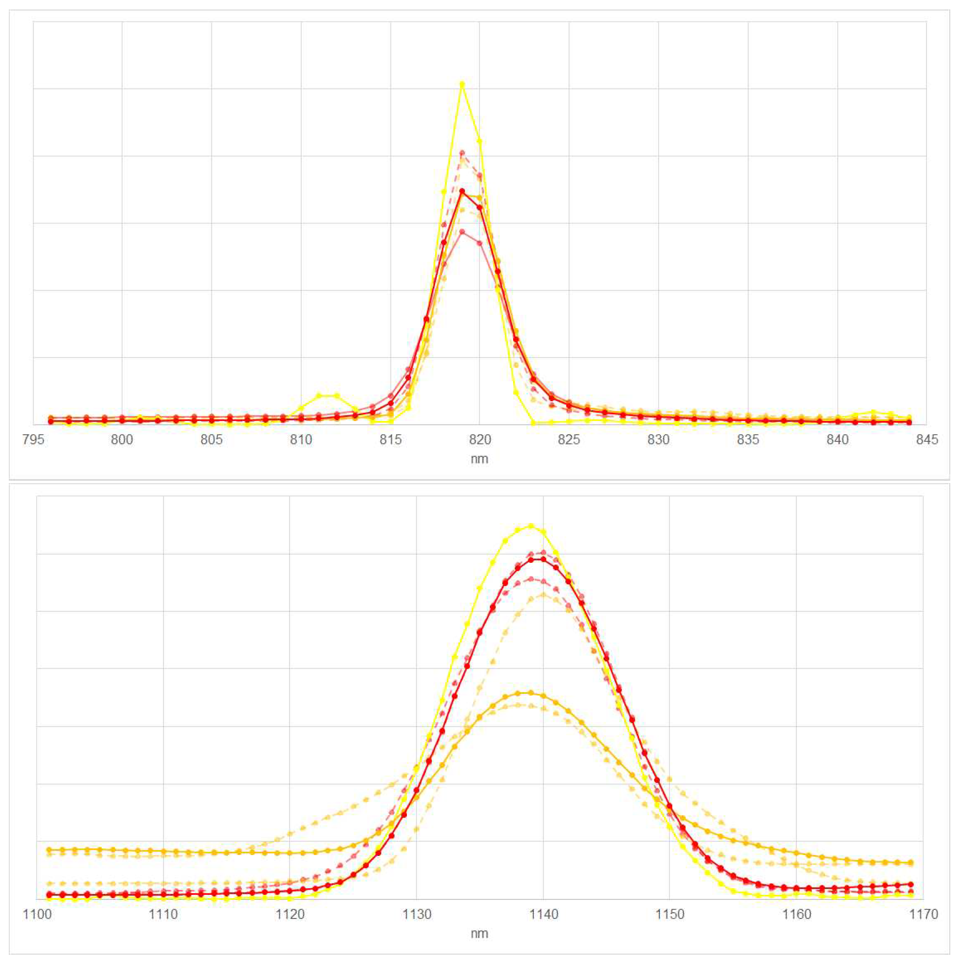
Figure 4.
Atmospheric transmission for an urban mid-latitude summer atmosphere at nadir with a maximal (green), a default (yellow) and a minimal (blue) water vapour for VIS/NIR (top) and SWIR (bottom) in the considered ranges.
Figure 4.
Atmospheric transmission for an urban mid-latitude summer atmosphere at nadir with a maximal (green), a default (yellow) and a minimal (blue) water vapour for VIS/NIR (top) and SWIR (bottom) in the considered ranges.
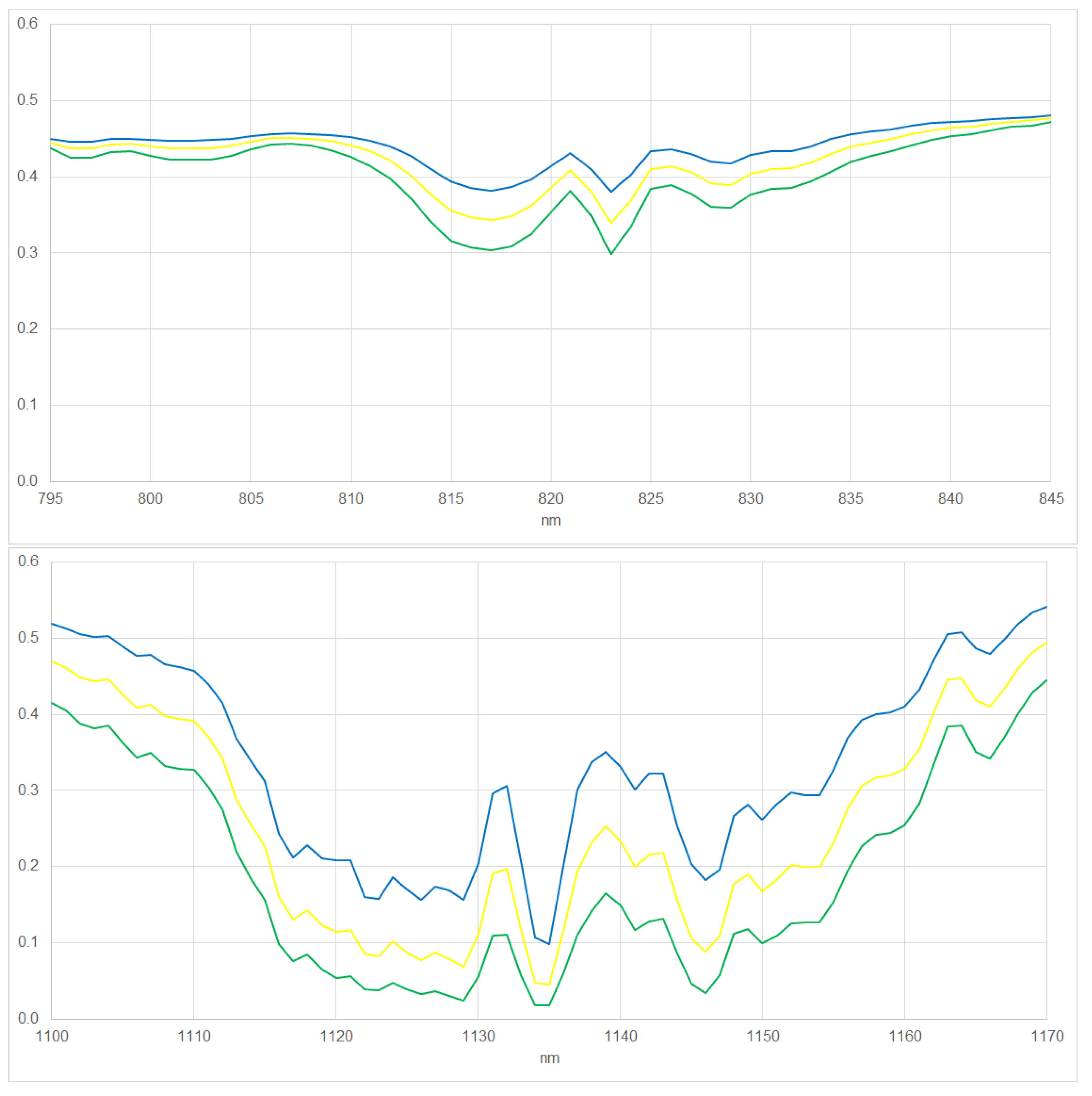
Figure 5.
HPS reference spectrum at 1nm resolution (red line) and image spectra at EnMAP resolution resulting for different shifts (not red lines) for VIS/NIR (top) and SWIR (bottom).
Figure 5.
HPS reference spectrum at 1nm resolution (red line) and image spectra at EnMAP resolution resulting for different shifts (not red lines) for VIS/NIR (top) and SWIR (bottom).
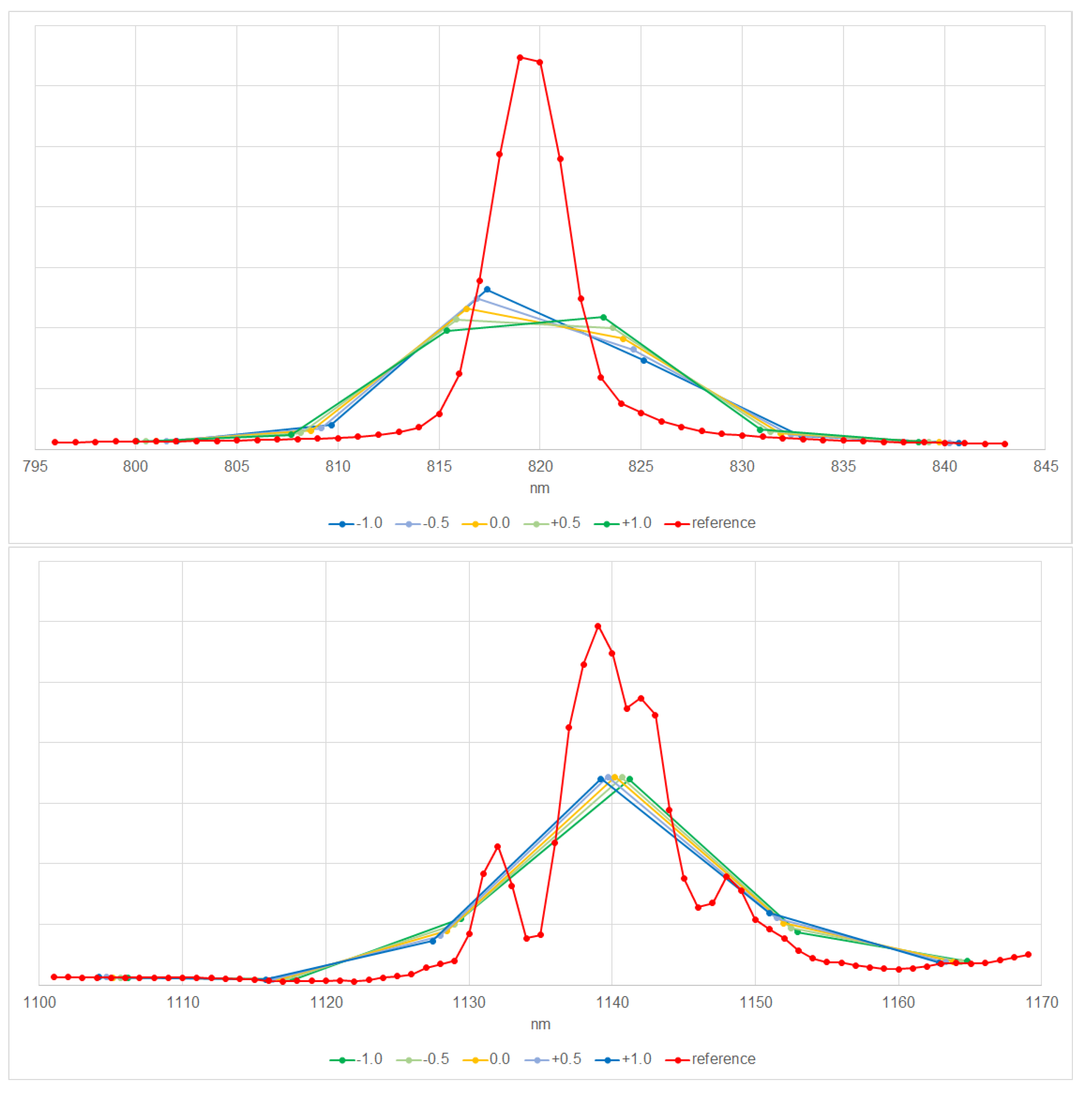
Figure 6.
Image and reference spectra for the scenarios when using the center pixel, pixel with maximum signal, sum of the signals of all pixel, and optimum pixel for VIS/NIR (top) and SWIR (bottom).
Figure 6.
Image and reference spectra for the scenarios when using the center pixel, pixel with maximum signal, sum of the signals of all pixel, and optimum pixel for VIS/NIR (top) and SWIR (bottom).
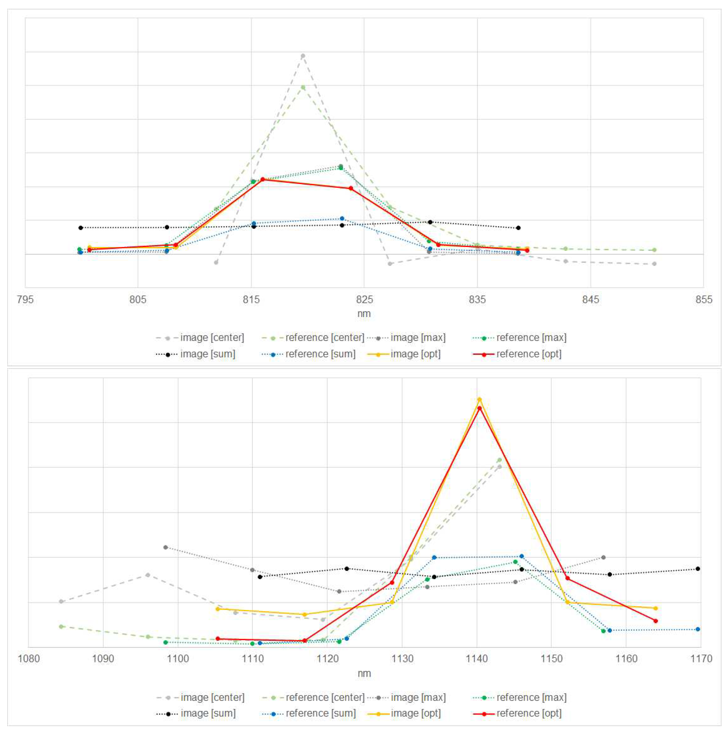
Figure 7.
Influence of the number of pixels on the approach Optimum. Fitting error (line 1 and 3 of diagrams) as well as estimated shift (in nm) (line 2 and 4 of diagrams) (y-axis) considering a smaller (line 1 and 2 of diagrams) or larger (line 3 and 4 of diagrams) amount of summed image spectra (x-axis) for VIS/NIR (left) and SWIR right).
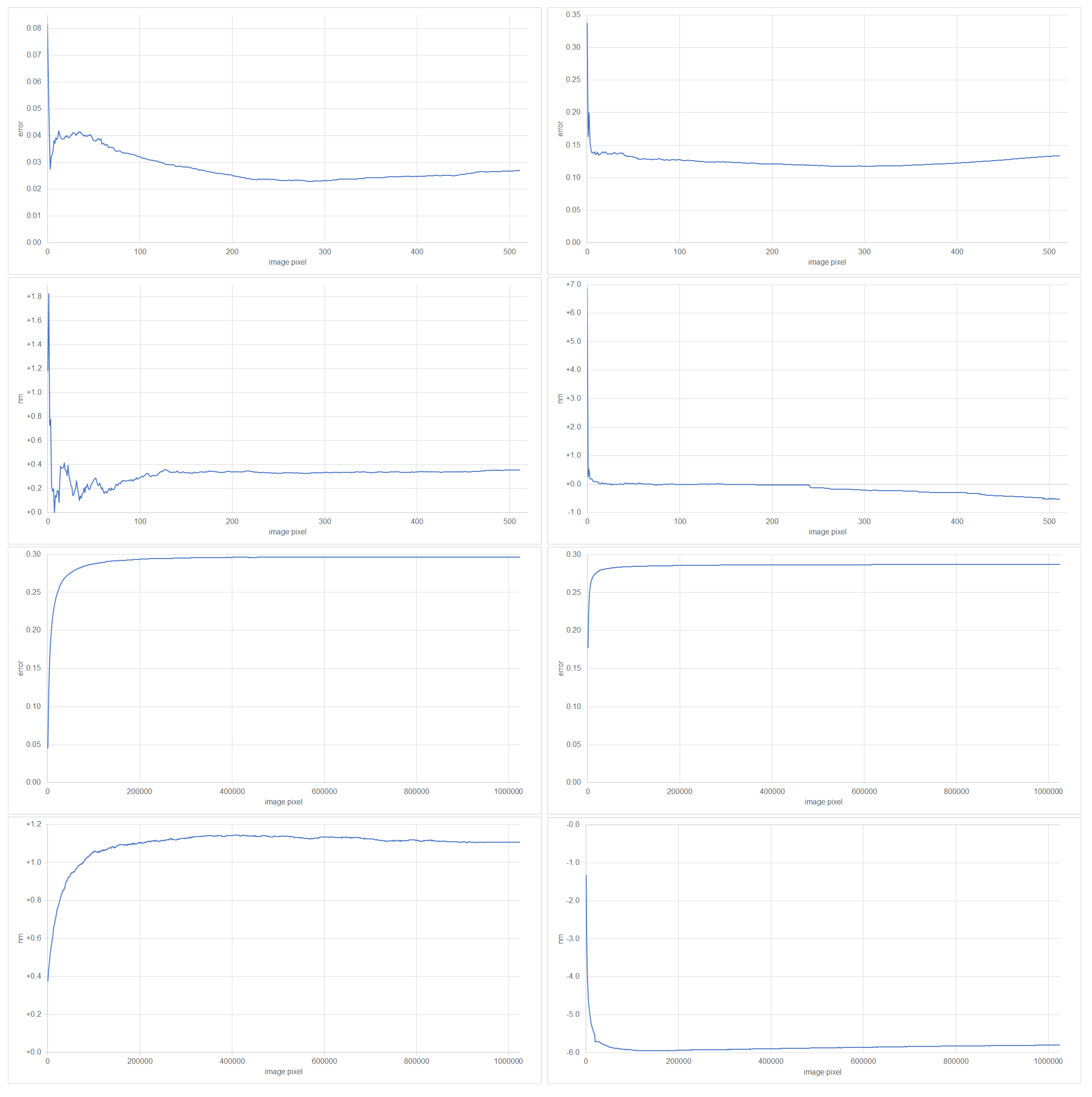
Figure 8.
Influence of noise on the estimation for VNIR (left) and SWIR (right). The differences of observed shifts compared to the shifts of the related noisy reference spectra given on the x-axis for observed errors given on the y-axis (see text for full description). Changes of green to olive and blue to purple illustrate the maximal variety of shifts of the noisy reference spectra resulting in the observed errors and shifts. A full green hue would be related to a negative shift of nm and a full blue hue to a positive shift of nm. Full red color illustrates the non-existence of shifts of noisy reference spectra resulting in the observed errors and shifts.
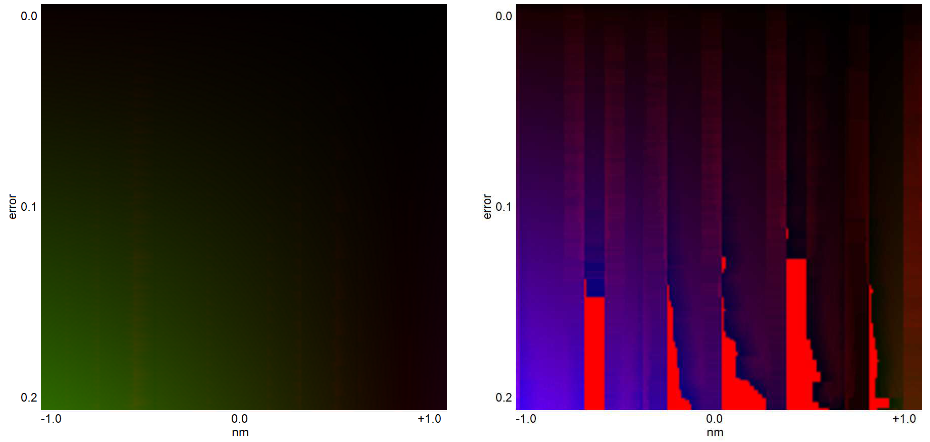
Figure 9.
Integrated signals in the range of bands with respect to the peaks of the emission at 819nm for VIS/NIR (left) and 1,139nm for SWIR (right). EnMAP data © DLR 2022. All rights reserved.
Figure 9.
Integrated signals in the range of bands with respect to the peaks of the emission at 819nm for VIS/NIR (left) and 1,139nm for SWIR (right). EnMAP data © DLR 2022. All rights reserved.
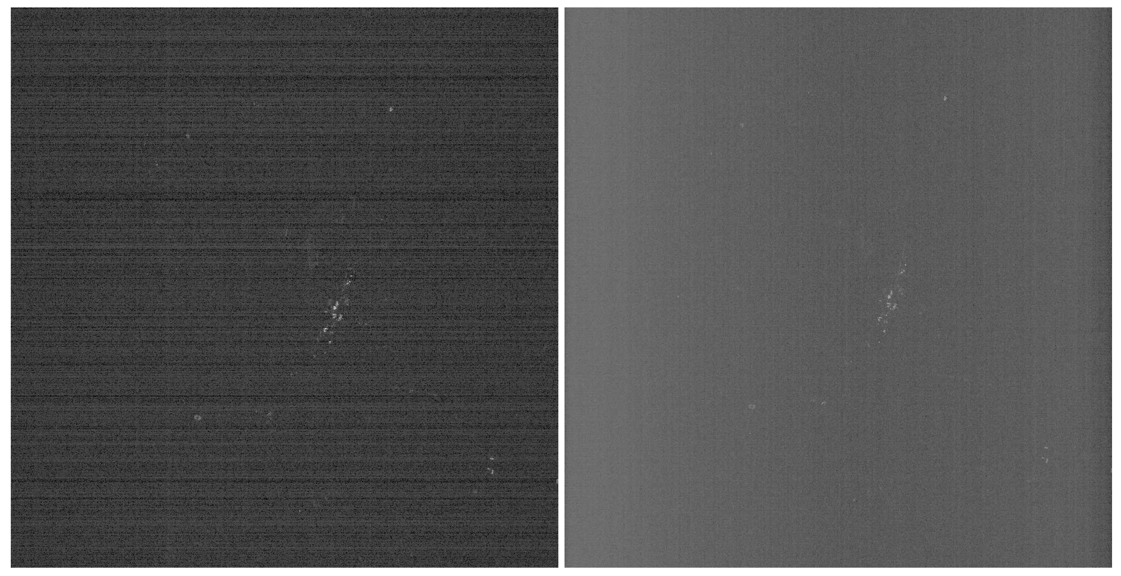
Figure 10.
Per-pixel center wavelengths based on laboratory calibrations (blue), as estimated considering the complete sensor (red), and the best fitted two of four parts of the sensor (magenta) for VIS/NIR (top) and SWIR (bottom).
Figure 10.
Per-pixel center wavelengths based on laboratory calibrations (blue), as estimated considering the complete sensor (red), and the best fitted two of four parts of the sensor (magenta) for VIS/NIR (top) and SWIR (bottom).
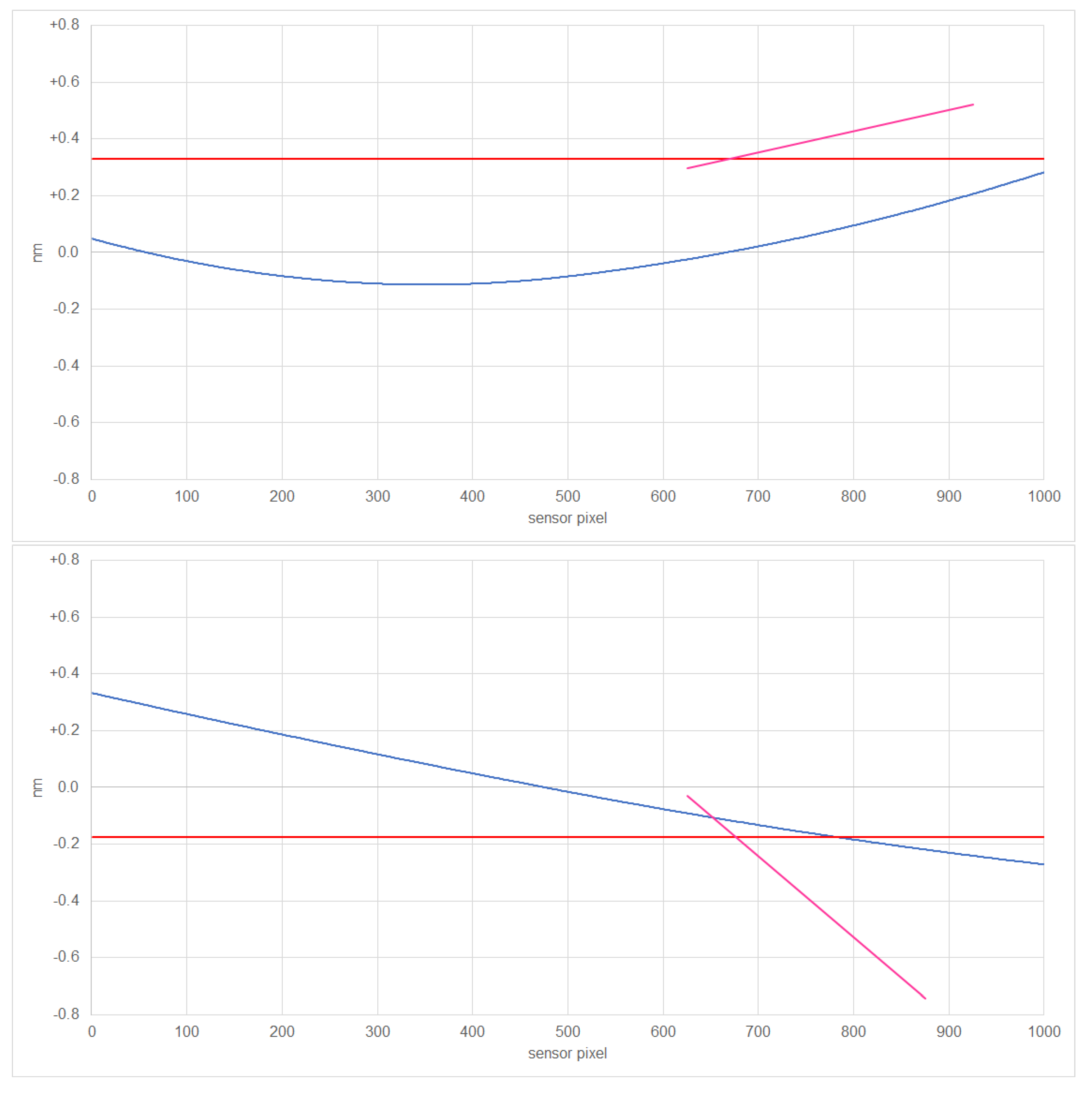
Figure 11.
Identified lighting types and temperatures based on VIS/NIR (left top and left bottom for differentiation of types of LED) and SWIR (right top and right bottom for temperatures).
Figure 11.
Identified lighting types and temperatures based on VIS/NIR (left top and left bottom for differentiation of types of LED) and SWIR (right top and right bottom for temperatures).
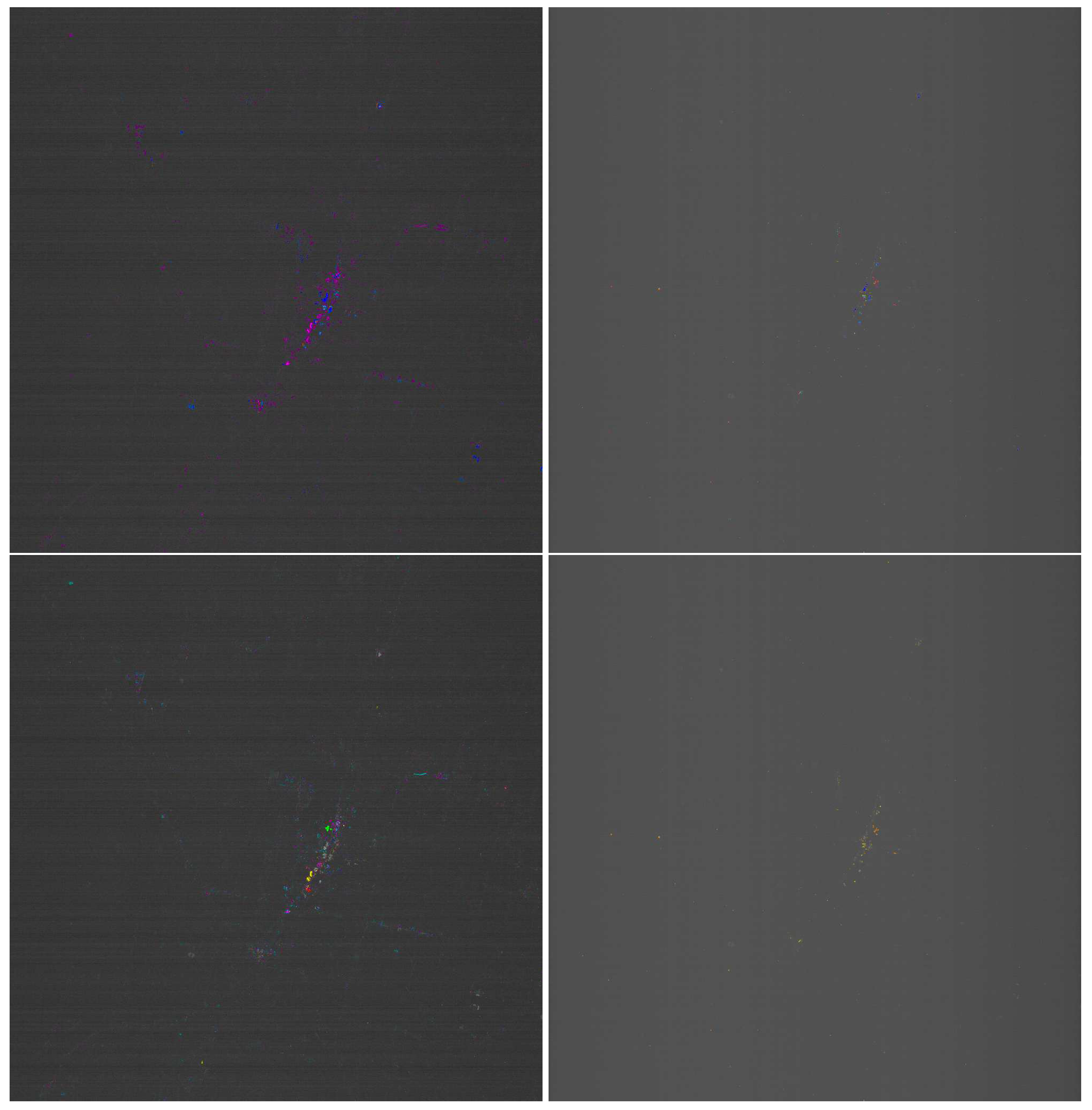
Figure 12.
Observed spectra (solid) and reference spectra by [8] (dashed). HPS (line 1), MH (line 2), FL (line 3, left), low temperature (line 3, right), LPS (line 4, left), high temperature (line 4, right), for VIS/NIR (left) and SWIR (right).
Figure 12.
Observed spectra (solid) and reference spectra by [8] (dashed). HPS (line 1), MH (line 2), FL (line 3, left), low temperature (line 3, right), LPS (line 4, left), high temperature (line 4, right), for VIS/NIR (left) and SWIR (right).
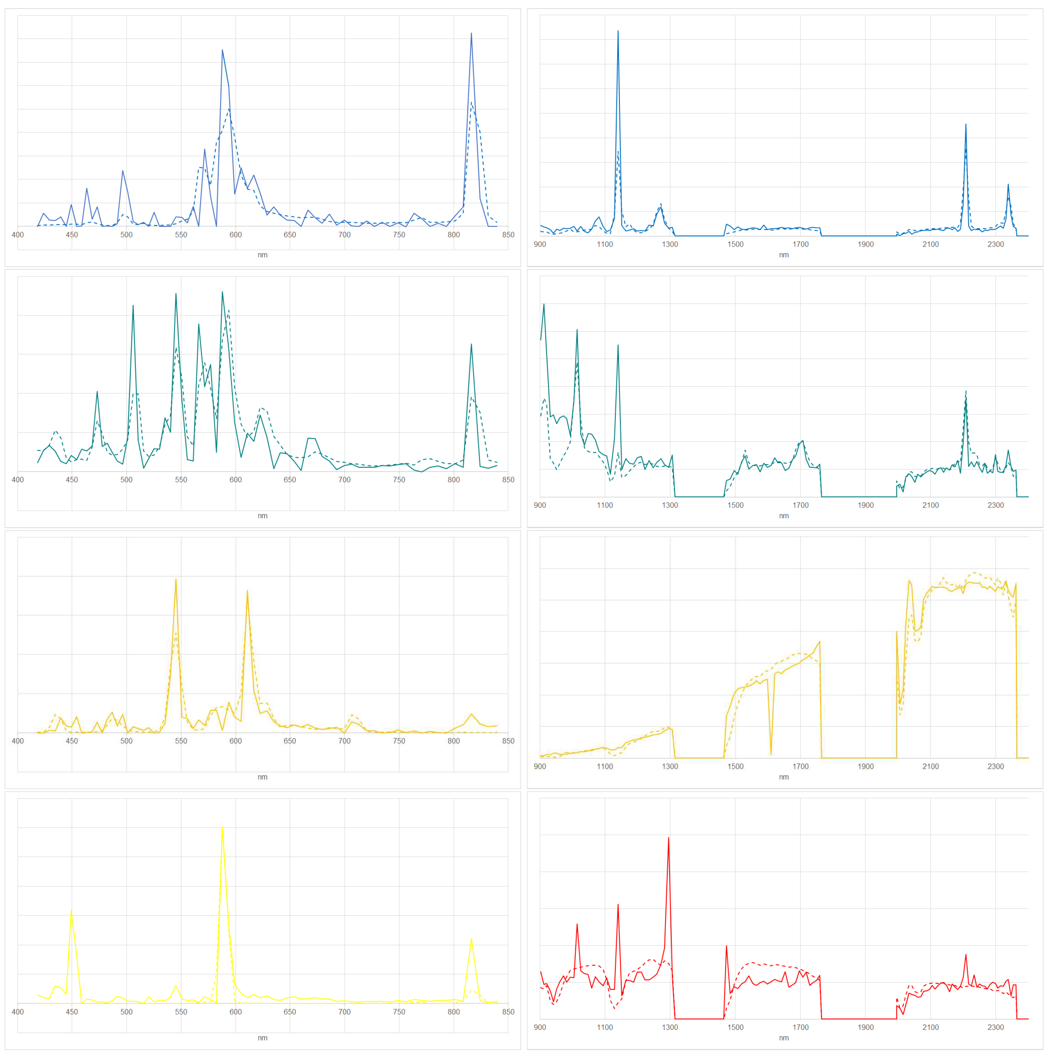
Figure 13.
Observed spectra (solid) and reference spectra by [8] (dashed). CW (line 1, left), NW (line 1, right), Blue LED (line 2, left), Green LED (line 2, right), Red LED (line 3, left), Yellow LED (line 3, right) for VIS/NIR.
Figure 13.
Observed spectra (solid) and reference spectra by [8] (dashed). CW (line 1, left), NW (line 1, right), Blue LED (line 2, left), Green LED (line 2, right), Red LED (line 3, left), Yellow LED (line 3, right) for VIS/NIR.
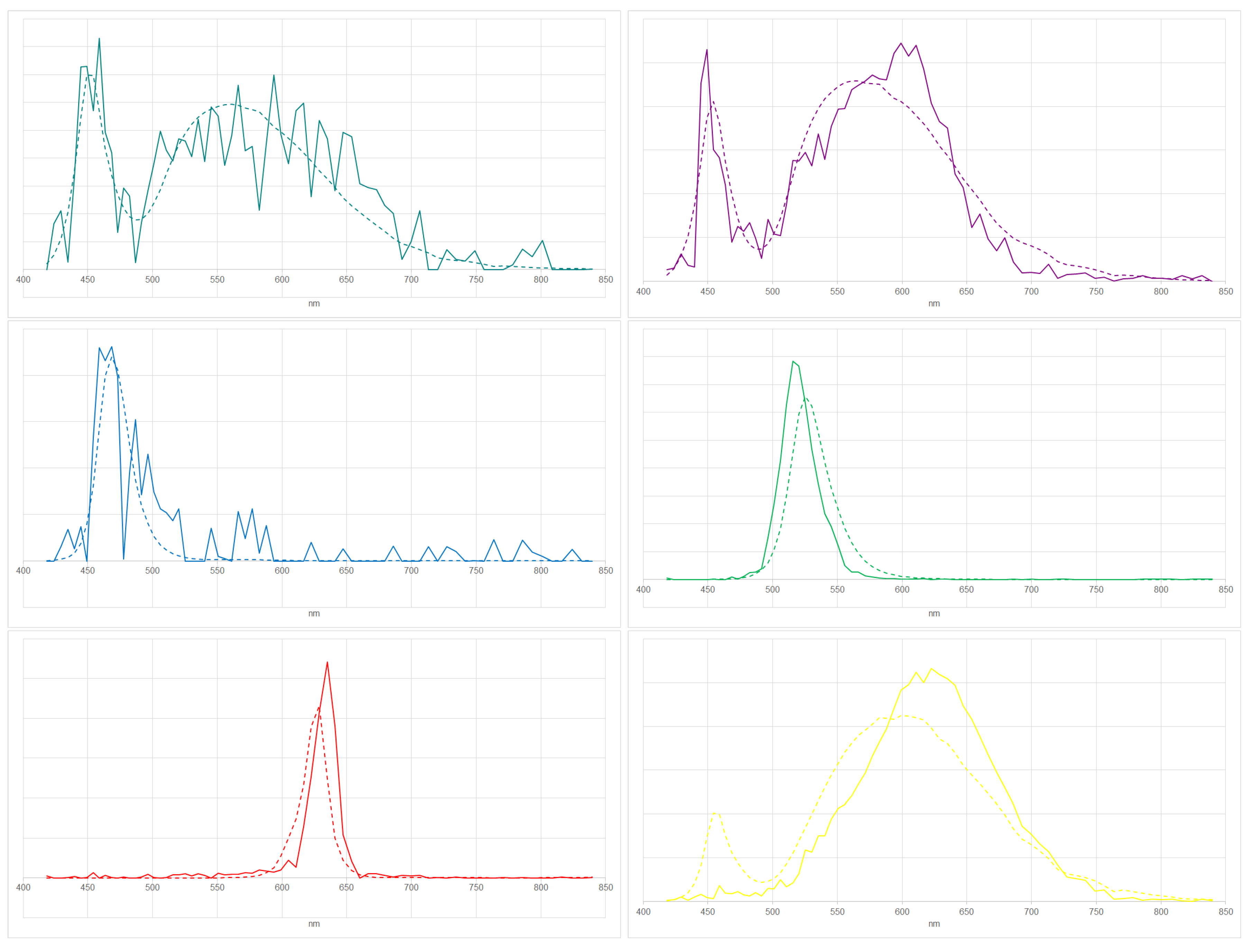

Table 1.
Uncertainties based on sensitivities and the influences of the assumptions A1 to A6 made.
| Description | VIS/NIR | SWIR | |
|---|---|---|---|
| sensitivity | to noise | ||
| A1 | lighting types | ||
| A2 | surface types | ||
| A3 | atmospheres | ||
| A4 | range of bands | ||
| A5 | distance metrics | ||
| A6 | image spectra selections | ||
| total | of sensitivity, A1, A2, A3 |
Table 2.
Identified lighting types based on VIS/NIR and SWIR. Error relates to the Euclidean distance of the fit against [8].
Table 2.
Identified lighting types based on VIS/NIR and SWIR. Error relates to the Euclidean distance of the fit against [8].
| error | error | ||||
|---|---|---|---|---|---|
| lighting type | color in figures | VIS/NIR | SWIR | VIS/NIR | SWIR |
| total | 8,819 | 451 | 2,006 | 448 | |
| HPS | dark blue | 430 | 48 | 165 | 48 |
| MH | light blue | 1,479 | 82 | 243 | 82 |
| MV | light green | 20 | 49 | 0 | 48 |
| QH | dark green | 5 | 6 | 0 | 6 |
| FL | orange | 174 | 26 | ||
| LPS | yellow | 8 | 8 | ||
| total LED | magenta | 6658 | 1557 | ||
| CW | cyan | 3311 | 509 | ||
| NW | magenta | 2437 | 740 | ||
| Blue | dark blue | 90 | 0 | ||
| Green | dark green | 69 | 1 | ||
| Red | dark red | 69 | 2 | ||
| Yellow | yellow | 682 | 305 | ||
| total INC/LIQ/PRES | dark red (VIS/NIR) | 45 | 111 | 15 | 108 |
| INC | magenta (SWIR) | 45 | 24 | 15 | 21 |
| LIQ | light magenta (SWIR) | 0 | 11 | 0 | 11 |
| PRES | dark magenta (SWIR) | 0 | 76 | 0 | 76 |
| Temperature | red-orange-yellow (SWIR) | 155 | 155 | ||
Table 3.
Estimated temperatures based on SWIR. Error relates to the Euclidean distance of the fit against emissions based on Planck’s law, separating and not separating the identified INC/LIQ/PRES.
Table 3.
Estimated temperatures based on SWIR. Error relates to the Euclidean distance of the fit against emissions based on Planck’s law, separating and not separating the identified INC/LIQ/PRES.
| error , separate temperature and INC/LIQ/PRES | error , separate temperature and INC/LIQ/PRES | ||||
|---|---|---|---|---|---|
| Temperature (K) | color in figures | yes | no | yes | no |
| 500 | red | 0 | 0 | 0 | 0 |
| 700 | red-orange | 1 | 1 | 1 | 1 |
| 900 | red-orange | 2 | 2 | 2 | 2 |
| 1100 | red-orange | 14 | 14 | 14 | 14 |
| 1300 | red-orange | 25 | 26 | 25 | 25 |
| 1500 | orange | 31 | 53 | 31 | 52 |
| 1700 | orange-yellow | 15 | 70 | 15 | 65 |
| 1900 | orange-yellow | 24 | 86 | 24 | 69 |
| 2100 | orange-yellow | 12 | 63 | 12 | 57 |
| 2300 | orange-yellow | 8 | 49 | 8 | 48 |
| 2500 | yellow | 23 | 87 | 23 | 84 |
Disclaimer/Publisher’s Note: The statements, opinions and data contained in all publications are solely those of the individual author(s) and contributor(s) and not of MDPI and/or the editor(s). MDPI and/or the editor(s) disclaim responsibility for any injury to people or property resulting from any ideas, methods, instructions or products referred to in the content. |
© 2023 by the authors. Licensee MDPI, Basel, Switzerland. This article is an open access article distributed under the terms and conditions of the Creative Commons Attribution (CC BY) license (https://creativecommons.org/licenses/by/4.0/).
Copyright: This open access article is published under a Creative Commons CC BY 4.0 license, which permit the free download, distribution, and reuse, provided that the author and preprint are cited in any reuse.


