1. Introduction
As climate change and environmental pollution become more prevalent and their effects on human well-being and the environment increase, the private sector plays a growing role in funding environmental projects [
1,
2]. In practice, measuring the financial contribution of contributors to environmental activities assists policymakers and/or planners in developing a better plan or stronger environmental policies. Many approaches have been adopted to support such activities, and contingent valuation (CV) is typically one of the most widely used methods of selection.
The contingent valuation is a survey-based method for estimating the economic value of non-marketable commodities and services. Because it uses a stated preference approach, consumers are explicitly questioned about their willingness to pay (WTP) for a good or service [
3]. The CV has been used to estimate the value of a wide range of goods and services, including clean air, clean water, biodiversity, and cultural heritage [
4,
5,
6,
7,
8]. It has also been used to estimate the costs of environmental damage, such as waste pollution and climate change [
3,
9,
10,
11]. Over the last two decades, CVM development has been centered on four main directions.
Firstly, developing better ways to represent goods and services to respondents. In the early days of the CV, scholars had trouble getting consumers to reply to questionnaires regarding their WTP for environmental goods and services. But as time has passed on, researchers have improved the manner in which they explain these products and services to respondents, which has increased the number of people who are willing to take part in CV surveys [
4]. Secondly, improving the way WTP is elicited from respondents. Scientists have improved their methods for eliciting WTP from respondents over time. For example, CV surveys used to frequently include open-ended question that asked respondents to state their maximum WTP. Open-ended questions, on the other hand, may be difficult for responders to answer, resulting in inconsistent responses [
12]. The researchers discovered that employing a different question structure, such as closed-ended questions that allow respondents to select from a list of specified WTP quantities, is more reliable. Thirdly, dealing with respondents’ strategic behavior. Respondents engage in strategic conduct when they attempt to affect the outcome of a CV survey by answering in a way that they believe will benefit them. Respondents, for example, may overestimate their WTP in order to obtain more money for themselves or their group. To deal with strategic behavior, researchers have developed a number of strategies, such as using random payment and providing respondents with enough information about the objective of the survey [
3]. Finally, addressing the issue of scope insensitivity. This issue refers to the case when respondents’ WTP for a good or service is unaffected by the quantity of the good or service available. Respondents may, for example, be willing to spend the same amount to save a small endangered species as they are to save a large endangered one. Researchers also found and used a range of strategies to deal with the scope insensitivity. For example, informing respondents about the shortage of the commodities or service might lessen the scope insensitivity.
Although CV has been much improved and widely accepted by scientists, agencies, policy-makers in many countries, it remains controversial to some degree [
3,
4,
12]. The CV is currently in development, and efforts to improve its accuracy and dependability are ongoing [
12]. In this regard, the purpose of the study is to develop and introduce a novel approach that combines contingent valuation and machine learning (CVML) to more accurately estimate households’ willingness-to-pay for environmental pollution reduction and/or climate change mitigation. This new method is expected to contribute to the literature on non-market valuation in environmental economics and sustainability studies.
2. Contingent valuation machine learning (CVML) framework
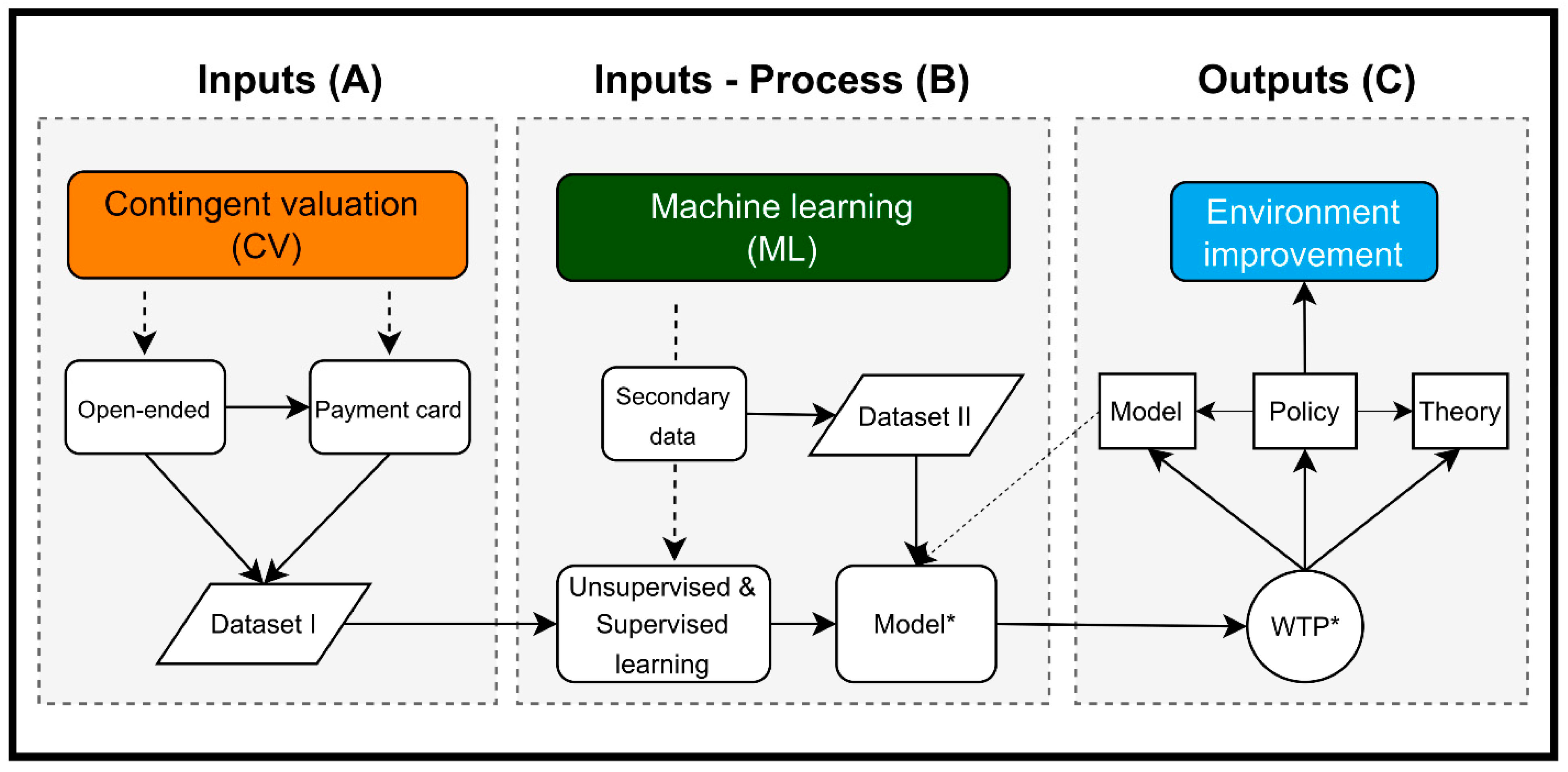
We develop and employ a contingent valuation machine learning (CVML) analytics system in this study (
Figure 1). This framework is briefly made up of three major components: inputs, processes, and outcomes. With the support of the machine learning method, the contingent valuation data is used as an input to develop the model (Block A). After the developed model has been well validated, it can be utilized to analyze data for the needs of the users (Block B). The estimated WTP would have numerous implications for model, theory, and policy (Block C).
2.1. Contingent valuation procedures
2.1.1. Open-ended
The open-ended question of contingent valuation method (CV) is a survey-based technique used to estimate the value of non-market goods and services. In this method, respondents are asked to state the maximum amount of money they would be willing to pay (WTP) for a particular good or service. The open-ended format is considered to be the most direct and accurate way to measure WTP, but it can be hard for respondents to answer this type of question.
The open-ended format has some advantages. First, the open-ended method does not provide respondents with any cues about what the value of the good or service might be. This helps to ensure that respondents’ responses are not influenced by their expectations of what the “correct” answer should be. Second, the open-ended method allows respondents to express their WTP in any amount, which can be more accurate than a dichotomous choice or payment card question, which typically only allows respondents to choose between two or three predetermined amounts. However, the open-ended question also has some disadvantages. First, it can be difficult for respondents to answer this type of question. They may not be familiar with the concept of WTP, or they may not be able to accurately estimate how much they would be willing to pay for a particular good or service. Second, the open-ended format can result in a large number of “don’t know” or “no response” answers. This can make it difficult to obtain a representative sample of respondents and to estimate the mean WTP for a good or service.
2.1.2. Payment card
In a CV survey, the payment card question presents respondents with a list of possible WTP amounts, and they are asked to circle the amount that best represents their WTP. The payment card method has several advantages over the open-ended question, which asks respondents to state their WTP without any guidance. The payment card format provides respondents with a frame of reference, which can help them to make more informed decisions. Additionally, the payment card method is less likely to produce outliers, which are extreme values that can skew the results of a survey. However, the payment card question also has some disadvantages. The list of possible WTP amounts may not be exhaustive, and respondents may not be able to find an amount that accurately reflects their WTP. Additionally, the payment card format can be more time-consuming for respondents to complete than the open-ended CV method.
2.2. Machine learning procedures
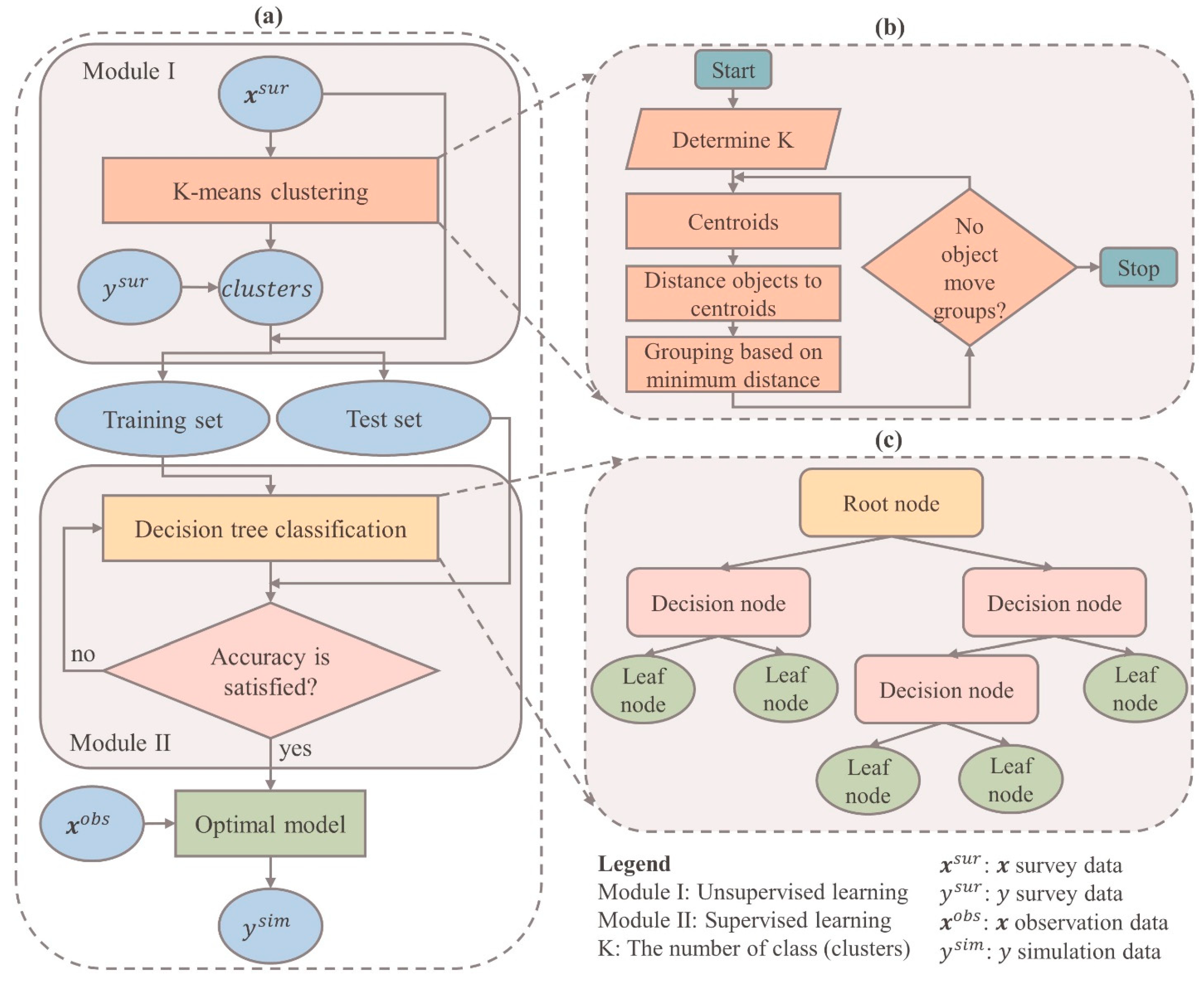
Typically, research endeavors are consistently troubled by issues related to data. The process of collecting data is a challenging task that demands significant investments of time and financial resources. To address this challenge, we propose an innovative hybrid machine-learning model that leverages a limited amount of survey data for prediction and data enrichment purposes. Our model comprises of two interconnected modules: Module I, an unsupervised learning algorithm, and Module II, a supervised learning algorithm. Module I is responsible for clustering the data (
) into groups based on common characteristics, thereby grouping the corresponding dependent variable (
) values as well. The output of Module I is the clustered data, which is then fed as input into Module II. In Module II, the output from Module I is utilized to construct a classification prediction model. Once Module II is built and its quality is assessed, it can be employed to predict the dependent variable (
) using the independent variables (
) sourced from previous studies or easily collected data.
Figure 2a illustrates the comprehensive framework, while
Figure 2b,c provide detailed insights into Module I and Module II, respectively.
2.2.1. K-means clustering algorithm (Module I)
K-means clustering is an unsupervised machine learning algorithm widely employed for grouping data points into distinct clusters based on their feature similarity [
13]. It operates by iteratively assigning data points to clusters and updating the cluster centroids. To categorize a given dataset into a predetermined number of clusters, the algorithm establishes K centroids, representing the center points of each cluster. It is crucial to position these centroids strategically to achieve an optimal solution globally. Therefore, the most favorable approach is to maximize the distance between centroids by placing them as far apart as possible. Next, every data point is assigned to the cluster whose centroid is closest to it. The algorithm then recalculates k new centroids, which serve as the average positions of all data points within each cluster. The data points are reassigned to the closest new centroid. This process is repeated either for a specific number of iterations or until consecutive iterations yield the same centroids [
14]. In the end, the objective of this algorithm is to minimize the total distortion or squared error. Distortion refers to the sum of distances between data points and their respective cluster centroids [
15]. The objective function (
) of K-means is given in Eq (1):
where
is the number of clusters,
is the number of data point,
is a Euclidean distance between a data point
and centroid
.
Figure 1b shows the algorithmic steps of the K-means clustering.
Step 1: Place K data items into the space to represent initial group centroids.
Step 2: Assign each data item to the group that has the closest centroid to that data item.
Step 3: Calculate the positions of K cluster centroids.
Step 4: Repeat Steps 2 and 3 until the positions of the centroids no longer change.
To determine optimal values of K, this study uses the Elbow method. This method is a popular technique used in K-means clustering to determine the optimal number of clusters, K, for a given dataset. It involves evaluating the within-cluster sum of squares (WCSS) metric, which quantifies the compactness or tightness of clusters [
16,
17,
18,
19]. The Elbow method proceeds by computing the WCSS for different values of K and plotting them against the number of clusters. The resulting plot exhibits a characteristic shape resembling an elbow. The idea behind the method is to identify the point on the plot where the rate of decrease in WCSS starts to diminish significantly, forming the “elbow”. This point indicates a trade-off between capturing more variance within clusters (smaller WCSS) and avoiding excessive complexity (larger K). The K value corresponding to the elbow point is often considered a reasonable choice for the number of clusters, striking a balance between model simplicity and cluster quality.
2.2.2. Decision tree classification algorithm (Module II)
Decision tree (DT) is a popular machine learning algorithm used for both regression and classification tasks [
20]. It is a supervised learning method that builds a predictive model in the form of a tree-based structure, where each internal node represents a feature or attribute, each branch represents a decision rule, and each leaf node represents a class label or a predicted value (see
Figure 1c). The goal of a DT classifier is to create an optimal tree that can efficiently partition the input data based on the feature values, ultimately leading to accurate predictions. The process of building a DT involves recursively splitting the data based on different features and their values, with the objective of maximizing the information gain or minimizing the impurity at each step [
20,
21]. There are different algorithms and strategies for constructing DT, such as Iterative Dichotomies 3 (ID3), Successor of ID3 (C4.5), and Classification and Regression Trees (CART) [
21]. These algorithms employ various criteria to determine the best splitting point, such as Entropy, Gini impurity, or Information gain [
22,
23]. The splitting criteria help in selecting the feature that provides the most discriminatory power and leads to the greatest reduction in impurity. In this study, the Gini index is used to evaluate the quality of a potential split when constructing a DT. It quantifies the probability of misclassifying a randomly selected element in a node if it were randomly assigned a class label according to the distribution of class labels in that node [
24]. Mathematically, the Gini index is calculated as follows:
where
is the probabilities of each class label in the node. The probabilities can be computed by counting the occurrences of each class label and dividing by the total number of data points in the node. When choosing a splitting criterion in a DT, the attribute or feature with the lowest Gini index or highest reduction in impurity is typically selected. A lower Gini index indicates a more homogeneous distribution of class labels within the resulting child nodes, leading to better separation and classification. By recursively applying this splitting process, the DT algorithm constructs a tree structure where each internal node represents a feature or attribute, each branch represents a decision rule based on a feature value, and each leaf node represents a predicted class label. In summary, the Gini index in the context of a DT is a measure of impurity that helps evaluate the quality of splits and guides the construction of an accurate DT model.
In general, DT is easy to understand and interpret, as the resulting tree structure can be visualized and explained. DT can handle both numerical and categorical features, and they can also handle missing values by assigning probabilities to different outcomes. Moreover, DT can capture non-linear relationships between features and target variables, and they can be used for feature selection, as the most important features tend to appear near the root of the tree.
2.2.3. Evaluation metrics
Precision, Recall, and F1 score are evaluation metrics commonly used in classification tasks to assess the performance of a machine learning model. They provide insights into the model’s accuracy, completeness, and overall effectiveness in making predictions [
25]. Precision is the measure of the model’s ability to correctly identify positive instances out of the total instances predicted as positive. It focuses on the accuracy of the positive predictions (Eq. 3).
where
(True Positives) represents the number of correctly predicted positive instances, and
(False Positives) represents the number of instances predicted as positive but are actually negative. Precision is particularly useful when the cost of false positives is high, and you want to minimize the number of false alarms or incorrect positive predictions. Recall, also known as sensitivity or true positive rate, measures the model’s ability to correctly identify positive instances out of the total actual positive instances. It focuses on the completeness of positive predictions (Eq. 4).
where
(False Negatives) represents the number of instances that are positive but predicted as negative. The Recall is especially valuable when the cost of false negatives is high, and you want to minimize the number of missed positive instances or false negatives. The F1-score combines Precision and Recall into a single metric that balances both measures. It is the harmonic means of Precision and Recall and provides a balanced evaluation of the model’s performance (Eq. 5).
The F1-score ranges from 0 to 1, where 1 represents perfect precision and recall, and 0 indicates poor performance in either precision or recall. The F1-score is particularly useful when we want to find a balance between precision and recall, as it considers both metrics simultaneously. These metrics are widely used together to assess the performance of a classifier. However, it’s important to note that their relative importance depends on the specific problem and the associated costs of false positives and false negatives.
2.2.4. Data
For this study, we utilized the same dataset on air pollution issues in Hanoi that was previously used by [
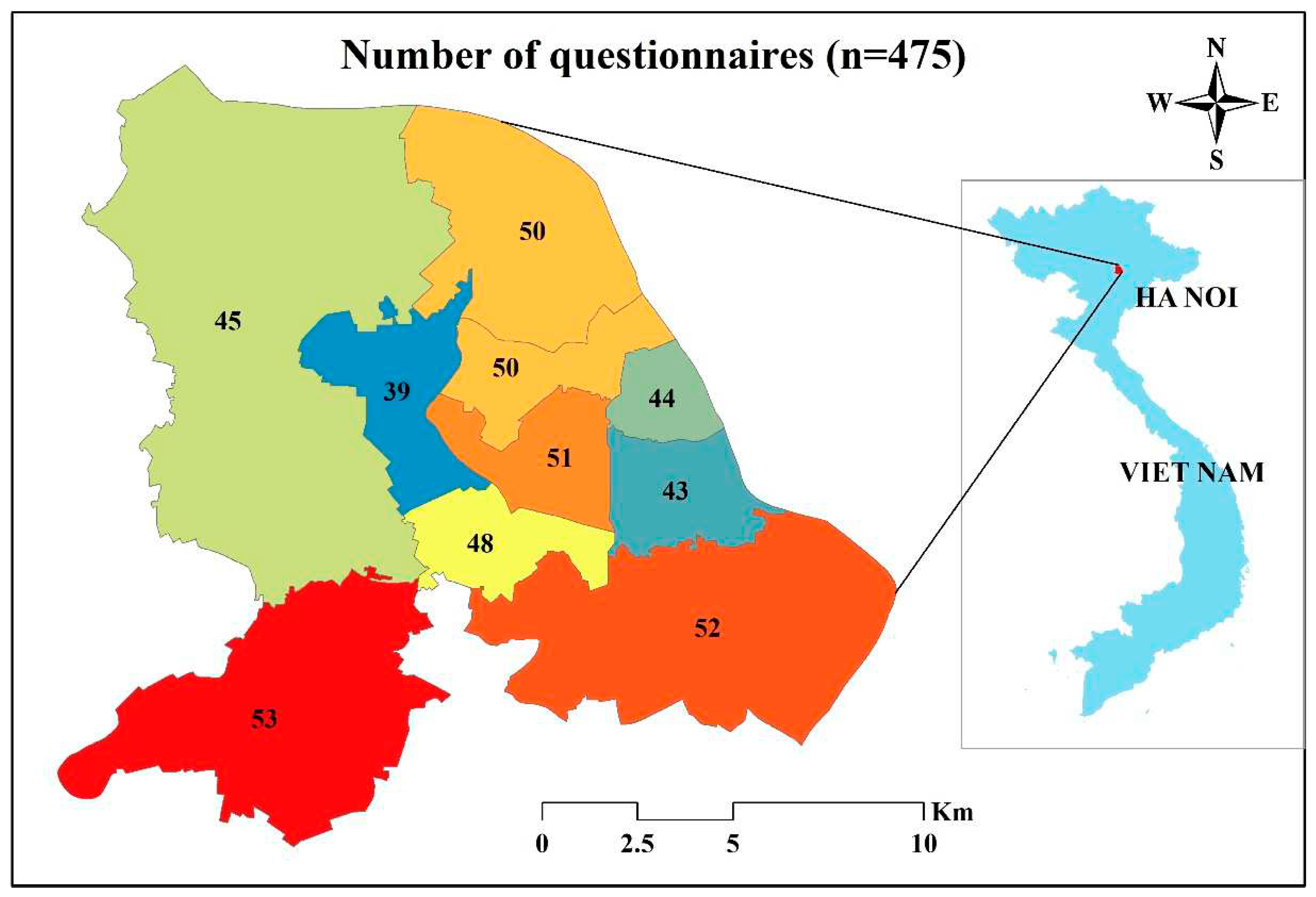
6] to build the CVML model. In November 2019, we chose to employ a face-to-face interview method to survey the residents of Hanoi over a period of three weeks. To ensure that there would be no potential confusion or misunderstandings between interviewers and prospective respondents, we conducted two pilot studies to thoroughly examine the questionnaire. Our goal was to guarantee clarity and understanding before proceeding with the official interviews. To recruit participants for our survey, we opted for a stratified random sampling technique. This approach, categorized as a probability sampling method, is renowned for its effectiveness in minimizing sample bias when compared to the simpler random sampling method. By utilizing stratified random sampling, we sought to achieve a more representative and accurate depiction of the population under study. Hanoi’s central urban area is comprised of 12 central districts. However, due to budget limitations, we focused our research on 11 districts, intentionally excluding the Long Bien district. The decision to omit Long Bien was based on its geographical location, as it is situated the furthest from the city center and is positioned on the opposite side of the Red River (
Figure 3). Within each of the selected districts, we proceeded to randomly select 40-50 local individuals from the main streets. In total, our efforts resulted in successfully conducting interviews with a sample size of 475 local individuals.
Table 1 provides the descriptive statistics for all variables used in this study. We have selected four independent variables (
) that possess the characteristics of being common and easily accessible. These variables will be utilized to examine their potential impact on the dependent variable (
), which represents the respondents’ willingness to pay. This dataset is used to train and test the CVML model which can be applied to predict willingness to pay by building independent variables from the available data (
).
3. Results of model development
3.1. The K-means cluster (Module I)
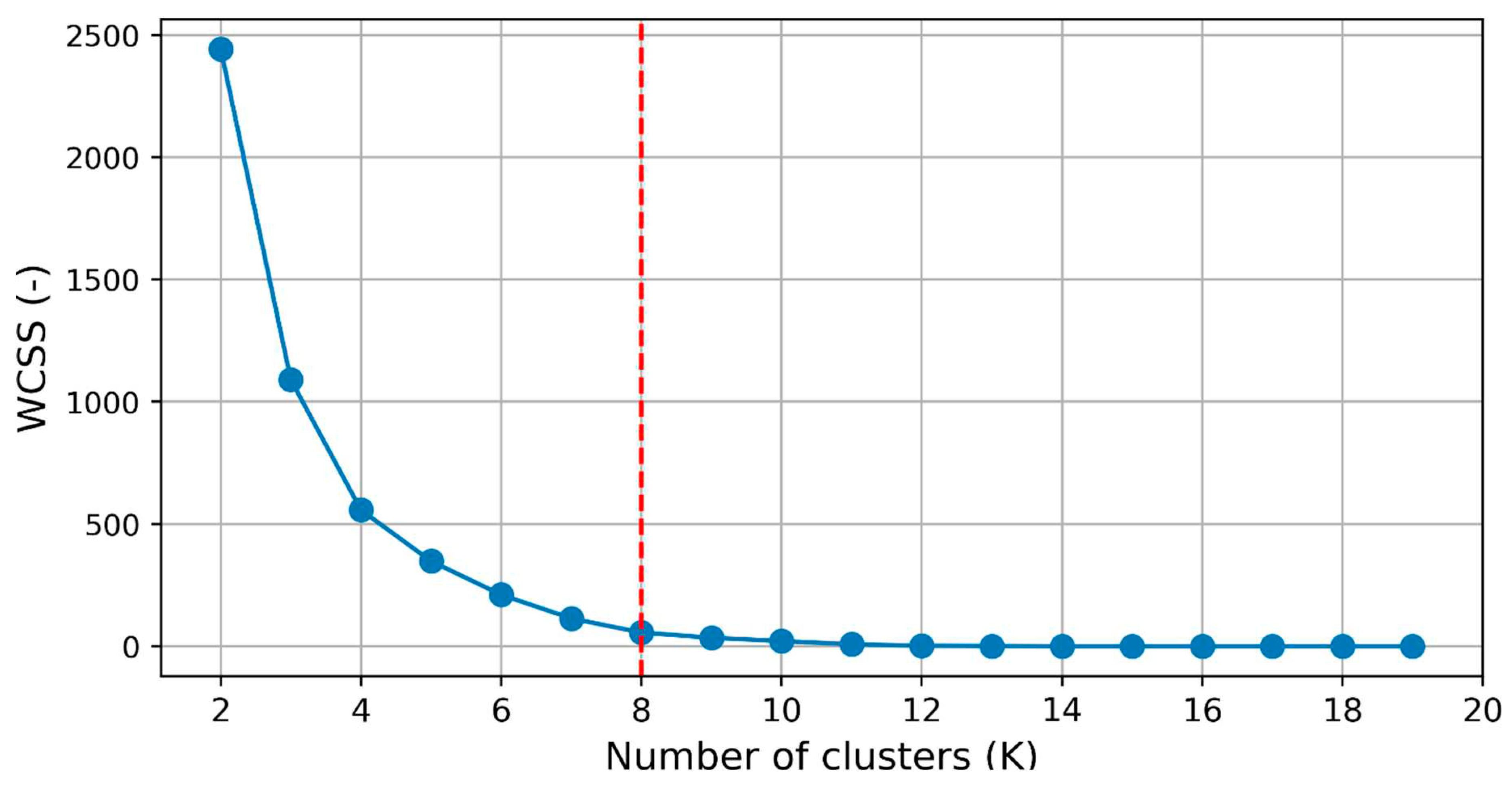
The
Figure 4 showcases the application of the elbow method to determine the ideal number of clusters (K) for a K-means clustering algorithm. This method aids in selecting the appropriate value of K by evaluating the variance explained as a function of the number of clusters. The plot depicts the number of clusters on the x-axis and the corresponding measure of variance or distortion on the y-axis. The distortion or within-cluster sum of squares (WCSS) is commonly used as the metric to assess the quality of the clustering. As the number of clusters increases, the WCSS tends to decrease since more clusters allow for a better fit of the data points. However, at a certain point, the rate of decrease in WCSS begins to diminish, resulting in a bend or "elbow" in the plot. In this specific figure, the elbow point is observed at K=8, indicating that the inclusion of additional clusters beyond this point does not significantly reduce the WCSS. The elbow represents a trade-off between capturing more detailed patterns within clusters and avoiding overfitting or excessive fragmentation. By selecting K=8, we strike a balance between granularity and simplicity, achieving a meaningful level of cluster differentiation without creating an overly complex or fragmented clustering solution. The elbow method provides a data-driven approach to guide the selection of the optimal number of clusters in K-means clustering, aiding in the interpretation and application of the results. It allows for efficient clustering by identifying the number of clusters that best capture the underlying structure of the data.
After applying the Elbow method, which determined that K=8 is the optimal number of clusters for the given dataset, K-means clustering was performed, resulting in eight distinct groups.
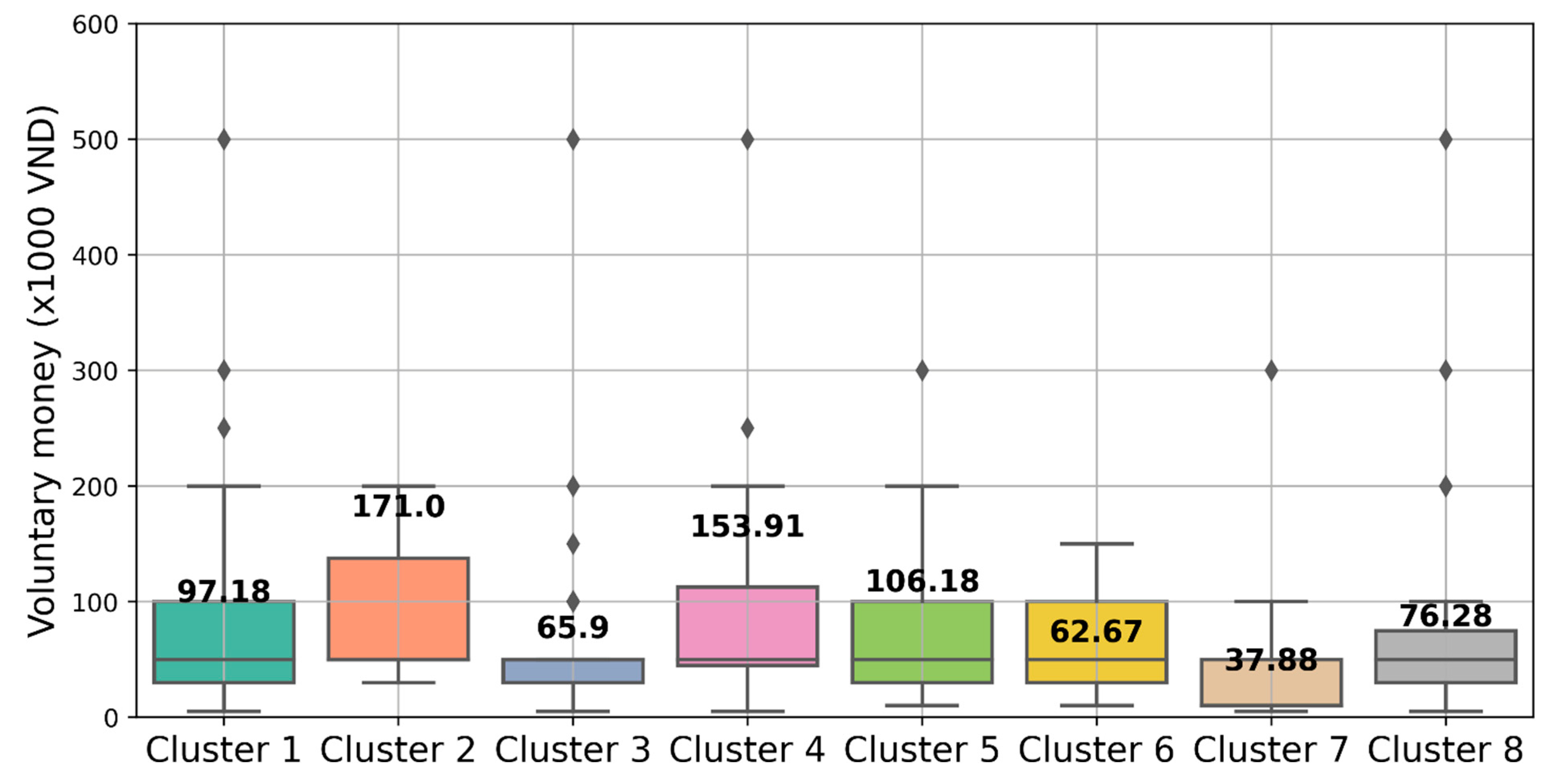
Figure 5 illustrates the average “voluntary money” value for each cluster. Notably, Group 4 stands out with a remarkable mean voluntary money value of 153.91 (×1000VND), indicating a strong inclination towards significant individual contributions. Similarly, Group 2 emerges as one of the highest contributing segments, with a mean value of 171.00 (×1000VND). In contrast, Group 7 exhibits the lowest mean value of 37.88 (×1000 VND), suggesting relatively lower levels of contribution compared to the other groups. The observed differences between groups are significant, reaching up to 4.5 times. This substantial variation highlights the potential for substantial errors if the mean method is solely used to estimate voluntary donations. Consequently, it becomes necessary to develop a predictive model to estimate the contribution amount for each group when estimating voluntary donations in a larger sample. By employing such a model, more accurate and reliable estimates can be obtained, accounting for the distinct contribution patterns exhibited by each group.
In Module II, the focus is on utilizing variable , which represents the input features, and variable , which represents the average voluntary money values of the eight groups. The goal is to construct a classification prediction model capable of predicting and estimating voluntary money when applied to a large number of samples.
3.2. The classification prediction model (Module II)
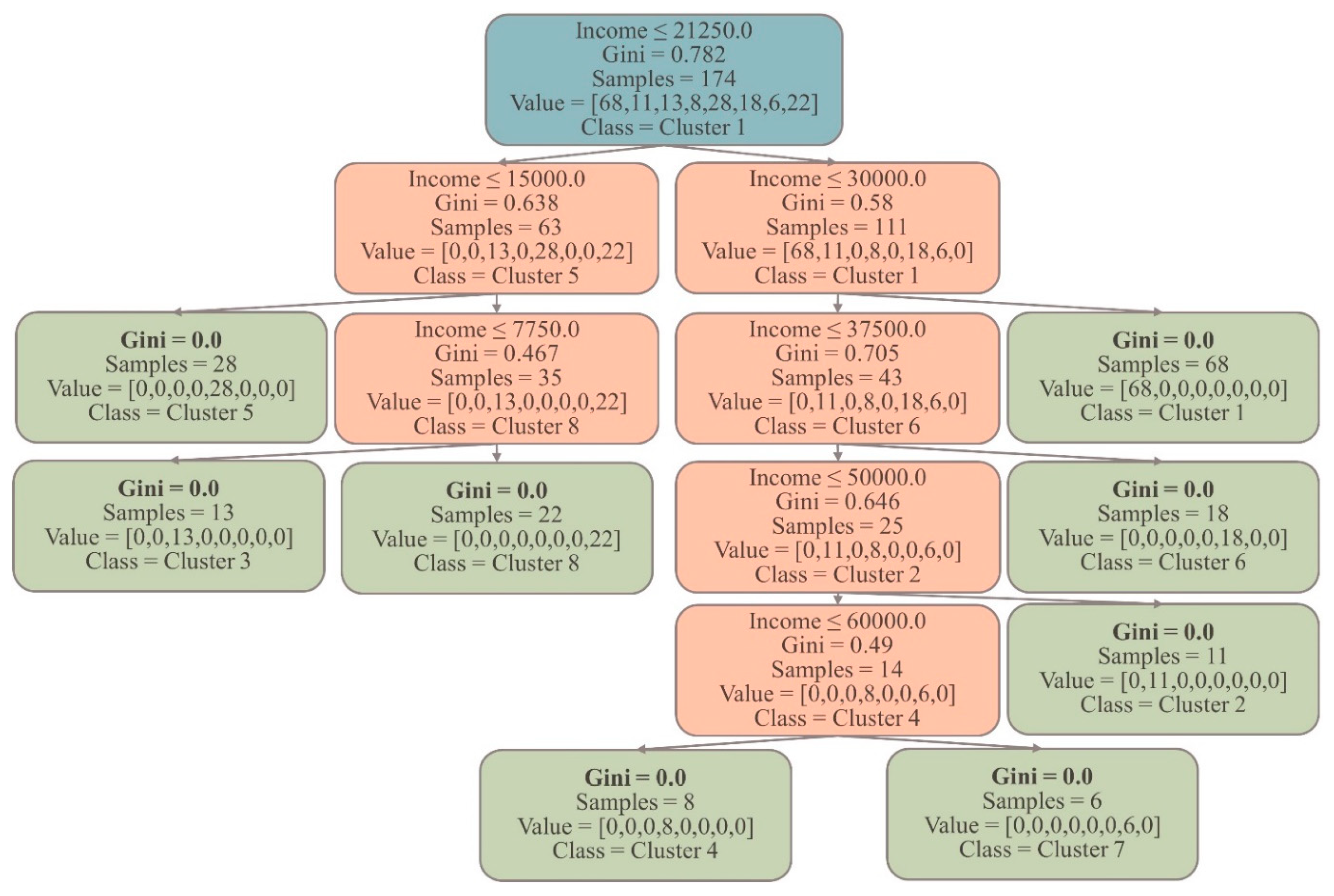
To train the DT model, 50% of the dataset is used. The model with a maximum depth of 5 is chosen as it provides sufficient complexity to classify all the groups in the dataset. This means that the DT, with its five levels of splits, can effectively capture the underlying patterns and relationships necessary to classify the samples into their respective groups. Importantly, after these five levels of splits, it is worth noting that all eight groups in the training dataset are successfully classified with a Gini index of 0. This signifies that the decision tree model has accurately captured the distinct characteristics and patterns of each group, resulting in pure nodes at the end of the fifth level. Achieving a Gini index of 0 for all eight groups indicates the absence of impurity or mixing of samples from different groups within their respective nodes (see
Figure 6). This showcases the model’s effectiveness in accurately separating and classifying the samples. By achieving a Gini index of 0 for all eight groups after five levels of splits, the decision tree classification model of Module II demonstrates its strong predictive power and ability to correctly assign new samples to their appropriate group based on their input features.
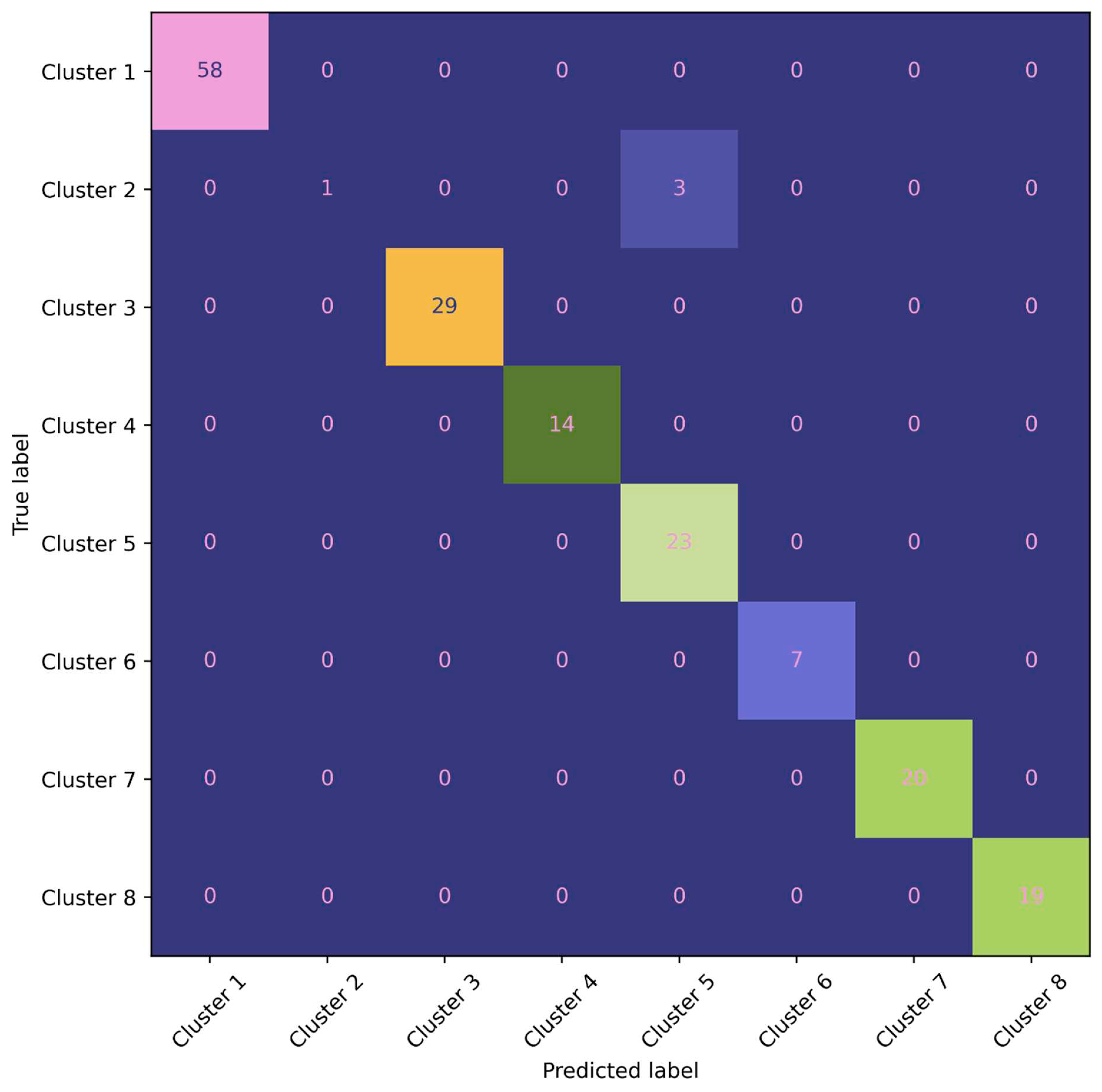
To evaluate the model’s performance and assess both its predictive ability and the presence of overfitting, we conduct testing on the test dataset (50% of the dataset). The test dataset serves as an independent set of samples that were not used during the model’s training process. During the testing phase, the model is applied to the test dataset, and the results are presented using a confusion matrix (
Figure 7). The confusion matrix provides a comprehensive overview of the model’s performance by showing the counts of true positive, true negative, false positive, and false negative predictions.
In this detailed confusion matrix, we explore the performance of a classification model designed to classify data into eight distinct classes. The matrix provides valuable insights into the accuracy and efficacy of the model’s predictions. The rows in the matrix correspond to the actual classes, while the columns represent the predicted classes. Each cell in the matrix indicates the number of instances that belong to a specific true class and were classified as a specific predicted class. This visual representation allows us to analyze both correct and incorrect predictions across the various classes. The diagonal cells from the top-left to the bottom-right of the matrix display the number of correctly classified instances for each class. Higher values along this diagonal indicate a higher level of accuracy and effectiveness in the model’s predictions.
Upon evaluating the model’s performance on the test dataset, we observe that the model successfully predicts all clusters, except for cluster 2, which has only one correct prediction out of four values. This indicates that the model performs well in accurately classifying most of the clusters, but there may be some challenges or complexities specifically associated with cluster 5.
Table 2 presents the Precision, Recall, and F1-score of the decision tree (DT) model on the test set, providing a detailed evaluation of its performance Clusters 1, 3, 4, 6, 7, and 8 demonstrate perfect precision, recall, and F1-scores of 1, indicating accurate predictions for all instances within these clusters. They have respective instance counts of 58, 29, 14, 7, 20, and 19. Cluster 2 exhibits a lower recall of 0.25, indicating that only 25% of the values that need to be forecasted are correctly predicted by the model. The precision is reported as 1, indicating that all the predictions made for this cluster are accurate. Cluster 2 comprises only 4 instances. Cluster 5 shows a precision of 0.88, indicating that 12% of the predictions made for this cluster are mistakenly classified by other groups. However, the recall is 1, indicating that all the values that belong to this cluster are correctly predicted. By analyzing these performance metrics, we can gain insights into the strengths and weaknesses of the decision tree model’s classification performance for each specific cluster. These metrics enable us to assess the model’s accuracy and identify areas for potential improvement, such as addressing the misclassification issue in Cluster 2 and 5 to improve precision.
Overall, the decision tree model demonstrates a high average accuracy of approximately 98%. The model successfully predicts most clusters accurately, with only clusters 2 and 5 experiencing lower accuracy. The primary reason for this could be attributed to the small number of samples available for these clusters, resulting in limited information and potential difficulties in capturing their underlying patterns. The limited sample size in clusters 2 and 5 may lead to insufficient representation of their characteristics during the model training process. As a result, the model might struggle to generalize well for these clusters, leading to lower accuracy in their predictions. To address this issue and improve the accuracy for clusters 2 and 5, it is recommended to acquire additional training and test data specifically targeting these clusters. By incorporating more samples, the model can gain a better understanding of their unique patterns and enhance its predictive performance.
4. Testing the applicability of the CVML method
The study found that by utilizing only four commonly available independent variables (
) the CVML model demonstrated promising results in predicting the respondents’ willingness to pay, as indicated by the test dataset (
Section 2.2.2). This outcome presents an opportunity to apply the CVML model for predicting willingness to pay by leveraging existing data, thereby reducing the time and costs associated with conducting extensive surveys.
In this study, we aim to apply the CVML model to predict the respondents’ willingness to pay using available data (
published by [
26]. Additionally, we will compare the predicted values obtained from the CVML model with the estimated results generated by the CV method, as presented in the study conducted by [
6,
27,
28]. It is important to note that both the CVML model and the CV method utilize the same dataset for their analyses. By comparing the predicted values from these two approaches, we can assess the accuracy and efficiency of the CVML model in predicting willingness-to-pay in relation to the established CV method, providing valuable insights into the predictive capabilities of the CVML model using the available dataset.
In the published dataset titled “A Data Collection on Secondary School Students’ STEM Performance and Reading Practices in an Emerging Country” [
26], there are a total of 42 variables and 4,966 respondents. For the purpose of the CVML model, we filter out four specific variables from this dataset. We then proceed to standardize the values of these variables to ensure they are on the same scale as the training dataset. After filtering and standardization, the resulting dataset consists of 714 matching lines, with the four variables of interest referred to as
. These variables are now ready to be used as inputs for the CV and CVML models to predict the respondents’ willingness to pay.
According to the CV method, the estimated willingness to pay for reducing air pollution ranged from
$4.6 to
$6.04 per household [
6]. With a total of 714 households, the estimated total for air pollution control would range from
$3,284.4 to
$4,312.56 (with an average of
$3,798.48). On the other hand, the prediction of the CVML method yielded a result of
$3,984.12, which is 4.8% higher than the average estimated by the CV method. This indicates that the CVML method predicted a slightly higher value for willingness to pay compared to the CV method’s average estimation. The difference in the predicted values suggests that the CVML model may have accounts for additional factors or incorporated different variables, leading to a slightly higher prediction. This finding highlights the potential of the CVML model to provide improved predictions compared to the traditional CV method in estimating willingness to pay for air pollution control as well as other fields.
In general, the accuracy of CVML models is comparable to the CV method, as shown in this case. However, the CVML model has the potential to become more reliable when applied to larger datasets. One of the significant advantages of the CVML model is its efficiency, primarily due to its reliance on simple and commonly available input data. This means that public sources and data from previous studies can be utilized, reducing the need for extensive and costly data collection efforts.Moreover, the data required for the CVML model is fundamental and can be easily disseminated, aligning with the digital data development strategies of certain developing countries like Vietnam. This compatibility with basic data sources facilitates the implementation and scalability of the CVML model, making it a powerful tool for socioeconomic studies. Overall, the CVML model offers a promising approach that combines accuracy and efficiency, especially when applied to larger datasets and in conjunction with the digital data strategies adopted by developing countries.
5. Conclusion
Contingent valuation has been extensively used because of its usefulness, yet its limitations make it less powerful. This study is one of the first efforts to further advance and advocate using the contingent valuation machine learning (CVML) analytics method. To illustate, we used the air pollution dataset from Hanoi, the K-means cluster (modle I) and decision tree model (model II) to develop a desired model. This model was then used to estimate WTP value for the targeted data. A high accuracy in prediction of the developed model implies that CVML can improve the WTP estimate [
4,
12] while a high capability of making use of the open-data source suggests that the method can help users reduce costs or save resources [
29]. This does mean that users, particularly those from low-resource countries, could benefit immensely from the approach. With these apparent attributes that CVML provides, the method could be potentially widely used in a wide range of domains in science. In practices, the method can further support the decision-makers to improve the financial to maintain and/or support many environmental programs in the coming time.
Author Contributions
Conceptualization, V.Q.K and D.T.T; methodology, V.Q.K and D.T.T; software, V.Q.K and D.T.T; validation, V.Q.K and D.T.T; formal analysis, V.Q.K and D.T.T; resources, V.Q.K and D.T.T; data curation, V.Q.K and D.T.T; writing—original draft preparation, V.Q.K and D.T.T; writing—review and editing, V.Q.K and D.T.T; visualization, V.Q.K and D.T.T; supervision, V.Q.K; All authors have read and agreed to the published version of the manuscript.
Funding
This research received no external funding.
Data Availability Statement
not applicable.
Acknowledgments
We would also like to express our sincere thanks to anonymous reviewers. who provide constructive comments to improve the paper’s quality
Conflicts of Interest
The authors declare no conflict of interest.
References
- Atteridge, A. Will Private Finance Support Climate Change Adaptation in Developing Countries ? Historical Investment Patterns as a Window on Future Private Climate Finance. Environment 2011, 1–38. [Google Scholar]
- Buso, M.; Stenger, A. Public-Private Partnerships as a Policy Response to Climate Change. Energy Policy 2018, 119, 487–494. [Google Scholar] [CrossRef]
- Champ, P.A.; Boyle, K.J.; Brown, T.C. A Primer on Nonmarket Valuation; Kluwer Academic Publishers, 101 Philip Drive, Norwell, MA 02061, U.S.A. 2017. [Google Scholar]
- Venkatachalam, L. The Contingent Valuation Method: A Review. Environ. Impact Assess. Rev. 2004, 24, 89–124. [Google Scholar] [CrossRef]
- Kamri, T. Willingness to Pay for Conservation of Natural Resources in the Gunung Gading National Park, Sarawak. Procedia - Soc. Behav. Sci. 2013, 101, 506–515. [Google Scholar] [CrossRef]
- Khuc, V.Q.; Nong, D.; Vu, P.T. To Pay or Not to Pay That Is the Question - for Air Pollution Mitigation in a World’s Dynamic City: An Experiment in Hanoi, Vietnam. Econ. Anal. Policy 2022, 74, 687–701. [Google Scholar] [CrossRef]
- Báez, A.; Herrero, L.C. Using Contingent Valuation and Cost-Benefit Analysis to Design a Policy for Restoring Cultural Heritage. J. Cult. Herit. 2012, 13, 235–245. [Google Scholar] [CrossRef]
- Khuc, V.Q.; Alhassan, M.; Loomis, J.B.; Tran, T.D.; Paschke, M.W. Estimating Urban Households’ Willingness-to-Pay for Upland Forest Restoration in Vietnam. Open J. For. 2016, 06, 191–198. [Google Scholar] [CrossRef]
- Wang, T.; Wang, J.; Wu, P.; Wang, J.; He, Q.; Wang, X. Estimating the Environmental Costs and Benefits of Demolition Waste Using Life Cycle Assessment and Willingness-to-Pay: A Case Study in Shenzhen. J. Clean. Prod. 2018, 172, 14–26. [Google Scholar] [CrossRef]
- Masud, M.M.; Junsheng, H.; Akhtar, R.; Al-Amin, A.Q.; Kari, F.B. Estimating Farmers’ Willingness to Pay for Climate Change Adaptation: The Case of the Malaysian Agricultural Sector. Environ. Monit. Assess. 2015, 187. [Google Scholar] [CrossRef]
- Nguyen, A.-T.; Tran, M.; Nguyen, T.; Khuc, Q. Using Contingent Valuation Method to Explore the Households’ Participation and Willingness-to-Pay for Improved Plastic Waste Management in North Vietnam. In Nguyen, A.T., Pham, T.T., Song, J., Lin, YL., Dong, M.C. (eds) Contemporary Economic Issues in Asian Countries: Proceeding of CEIAC 2022, Volume 2; Springer Nature Singapore, 2023; pp. 219–237.
- Carson, R.T. Contingent Valuation:A User’s Guide. Environ. Sci. Technol. 2000, 34, 1413–1418. [Google Scholar] [CrossRef]
- MacQueen, J. Some Methods for Classification and Analysis of Multivariate Observations. In Proceedings of the Proceedings of the 5th Berkley Symposium on Mathematical Statistics and Probability; 1967; pp. 281–297. [Google Scholar]
- Zˇalik, K.R. An Efficient k 0 -Means Clustering Algorithm. Pattern Recognit. Lett. 2008, 29, 1385–1391. [Google Scholar] [CrossRef]
- Rana, S.; Jasola, S.; Kumar, R. A Hybrid Sequential Approach for Data Clustering Using K-Means and Particle Swarm Optimization Algorithm. Int. J. Eng. Sci. Technol. 2010, 2. [Google Scholar] [CrossRef]
- Brusco, M.J.; Steinley, D. A Comparison of Heuristic Procedures for Minimum Within-Cluster Sums of Squares Partitioning. Psychometrika 2007, 72, 583–600. [Google Scholar] [CrossRef]
- J. A. Hartigan, M.A.W. Algorithm AS 136: A K-Means Clustering Algorithm. J. R. Stat. Soc. Ser. B Methodol. 1979, 28, 100–108. [Google Scholar]
- Krzanowski, W.J.; Lai, Y.T. A Criterion for Determining the Number of Groups in a Data Set Using Sum-of-Squares Clustering. Biometrics 1988, 44, 23. [Google Scholar] [CrossRef]
- Thorndike, R.L. Who Belongs in the Family? Psychometrika 1953, 18, 267–276. [Google Scholar] [CrossRef]
- Swain, P.H.; Hauska, H. Decision Tree Classifier: Design and Potential. IEEE Trans Geosci Electron 1977, GE-15, 142–147. [Google Scholar] [CrossRef]
- Mahesh, B. Machine Learning Algorithms - A Review. Int. J. Sci. Res. 2020, 18, 381–386. [Google Scholar] [CrossRef]
- Cheushev, V.; Simovici, D.A.; Shmerko, V.; Yanushkevich, S. Functional Entropy and Decision Trees. In Proceedings of the Proceedings of The International Symposium on Multiple-Valued Logic; 1998; pp. 257–262. [Google Scholar]
- Molala, R. Entropy, Information Gain, Gini Index—The Crux of a Decision Tree. Medium 2019, 1–8. [Google Scholar]
- Tangirala, S. Evaluating the Impact of GINI Index and Information Gain on Classification Using Decision Tree Classifier Algorithm. Int. J. Adv. Comput. Sci. Appl. 2020, 11, 612–619. [Google Scholar] [CrossRef]
- Goutte, C.; Gaussier, E. A Probabilistic Interpretation of Precision, Recall and F-Score, with Implication for Evaluation. Lect. Notes Comput. Sci. 2005, 3408, 345–359. [Google Scholar] [CrossRef]
- Vuong, Q.H.; La, V.P.; Ho, M.T.; Pham, T.H.; Vuong, T.T.; Vuong, H.M.; Nguyen, M.H. A Data Collection on Secondary School Students’ Stem Performance and Reading Practices in an Emerging Country. Data Intell. 2021, 3, 336–356. [Google Scholar] [CrossRef]
- Khuc, V.Q.; Vu, P.T.; Luu, P. Dataset on the Hanoian Suburbanites’ Perception and Mitigation Strategies towards Air Pollution. Data Br. 2020, 33, 106414. [Google Scholar] [CrossRef]
- Vuong, Q.-H.; Phu, T.V.; Le, T.-A.T.; Van Khuc, Q. Exploring Inner-City Residents’ and Foreigners’ Commitment to Improving Air Pollution: Evidence from a Field Survey in Hanoi, Vietnam. Data 2021, 6, 39. [Google Scholar] [CrossRef]
- Vuong, Q. The (Ir)Rational Consideration of the Cost of Science in Transition Economies. Nat. Hum. Behav. 2018, 2, 41562. [Google Scholar] [CrossRef]
|
Disclaimer/Publisher’s Note: The statements, opinions and data contained in all publications are solely those of the individual author(s) and contributor(s) and not of MDPI and/or the editor(s). MDPI and/or the editor(s) disclaim responsibility for any injury to people or property resulting from any ideas, methods, instructions or products referred to in the content. |
© 2023 by the authors. Licensee MDPI, Basel, Switzerland. This article is an open access article distributed under the terms and conditions of the Creative Commons Attribution (CC BY) license (http://creativecommons.org/licenses/by/4.0/).
