Concavity of the Conditional Mle for Logit Panel Data Models with Imputed Covariates

1. Introduction

Parameter estimation is a key goal of inferential statistics and most researchers attempt to fit data into models that would produce the best of all possible parameter estimates. The motivation behind the parameter estimation is to make inferences about a study population using sample information and this calls for very well spelled out ways of ensuring that unbiased and precise estimates are achieved in every parameter estimation technique so applied. During sample data collection researchers encounter missing values in the study variables, a problem that leads to complications in statistical analyses through inaccurate estimates that may eventually lead to incorrect inferences and policy actions.

Specifically, when the response variable is binary, problems of missing covariates are further compounded by the nonlinear treatment of the model specification. Studies on missingness and parameter estimation have shown that frequentist techniques of imputation result into biased estimates with significant loss of power [1,2,3]. This problem cuts across every model with no exception to the logit model for binary choice response variables and several studies have made attempts to come up with reliable imputation techniques for missing observations so as to reduce the estimates’ bias.

The logistic regression methods are often applied to procedures for describing the relationship between dichotomous outcome variables and other model covariates. The general method of estimating the logistic regression parameter is maximum likelihood and in a very general sense the maximum likelihood method yields values for the unknown parameters that maximize the probability of the observed set of data. Maximum likelihood (ML) method is occasionally prone to convergence problem, which occurs when the maximum likelihood estimates (MLE) do not exist. This subject of assessing the behaviour of MLE for logistic regression model is important, as the applications of the logistic model stretch far and wide across research disciplines. There exist numerous works which discuss convergence problem on logistic regression model by Cox et al. [4] or the bias reduction by Firth D., Anderson J.A. and Richardson C. [5, 6]. Other studies outline many assumptions of the distributions ML estimators resulting from bias reduction technique, and impact of varying sample size to MLE [7, 8].

S. Lee [9] notes that statistical inference based on the logistic regression model is highly dependent on the asymptotic properties of the maximum likelihood estimator. This means that under large sample situations, the sampling distribution of the maximum likelihood (ML) estimators for the logistic regression coefficients is asymptotically unbiased and normal. Conversely, in small samples, the asymptotic properties of maximum likelihood estimations may not hold due to biased estimates [9, 10]. Firth’s method has been introduced as one of the penalization techniques to correct or reduce the small sample bias of the ML estimators of the linear regression model [10, 11]. A comparison of the performance of the linear regression model based on maximum likelihood (ML) and Firth’s penalized maximum likelihood estimation methods was done by S. Lee. The results showed that, as compared with penalized maximum likelihood, the LR model based on asymptotic ML worked slightly better in terms of statistical power although the difference in performance was not practically important [9]. The present paper centers to evaluate the susceptibility of the Hessian matrix to different imputation techniques by comparing the magnitudes of the determinants obtained from the Hessian of the log-likelihood function with the imputed covariate vector.

This section gives the background of the study by introducing the concept of panel data econometrics and mentions various approaches to panel data models’ estimation where the conditional maximum likelihood estimation is mentioned as a solution to the incidental parameter problem in logistic panel data model.

Following the background introduction above, the rest of the paper is organized as follows. Section 2 focuses on the specification of the nonlinear binary choice panel data models. Section 3 highlights the incidental parameter problem in estimating logistic panel data model and shows how the conditional maximum likelihood approach circumvents it. In section 4 we discuss the parameter estimation for a logit panel data model in which the covariate vector is partitioned into sample present values and missing or imputed values. This discerns the impact of missingness on the Hessian of the conditional maximum likelihood estimator of nonlinear binary choice logistic model. Monte Carlo simulation results are also given and discussed in this section to assess the impact of missingness on the determinant of the Hessian matrix and the parameter estimates. Finally, section 5 gives the summary and conclusions from the study and consequently provide recommendations for further study, based on the key findings from this work.

2. Model Specification

2.1. Panel Data

Observing experimental subjects or units over a repeated number of times collates a set of data referred to as panel data which provides two kinds of information – cross-sectional and time series. This unique characteristic allows panel data to account for individual differences that are time-invariant by applying regression techniques which allow us to adequately take advantage of the different types of information.

The logit panel data model then develops from the logistic regression to model binary choice response variables which have had wide applications in almost all research fields that conduct pretest and posttest studies with the aim of discerning the impact of the test. As such, for $N$ units each observed $T$ times, we have a total of $N\times T$ observations made.

2.2. The Logit Panel Data Model

Consider a population unit $i$ is observed a time $t$ for a binary response variable $y$ against $K$ explanatory variables to which we specify a general fixed effects panel data model as a special case of the generalized longitudinal model in the form

(1)

In model (1), $\mathit{\beta }$ is a $1\times k$ vector of parameters of the $k\times 1$ column vector${\mathit{x}}_{\mathit{i}\mathit{t}}$. The parameter $c_i$ captures all individual-specific time-invariant characteristics of the study population unit. For fixed effects (FE) models the parameter $c_i$ is assumed to be correlated with ${\mathit{x}}_{\mathit{i}\mathit{t}}$leaving only $u_{it}~N(0,{\sigma }_y^2)$as the stochastic part of the model. Compounding $c_i$ and $u_{it}$ as a stochastic entity gives a random effects (RE) model. Let $y_{it}\in \left\{\mathrm{0,1}\right\}$ for all $i$ and $t$ where the values 0 and 1 consecutively represent the failure and success of an event occurring as described in the research experiment. We then have $y_{it}$ as a binary choice variable following a binomial distribution with probability of success for individual $i$ at time $t$ as $p_{it}=\mathrm{Pr}\left(y_{it}=1\right)=E\left(y_{it}|{\mathit{x}}_{\mathit{i}\mathit{t}},c_i\right)=F\left({\mathit{x}}_{\mathit{i}\mathit{t}}^{\mathit{\text{'}}}\mathit{\beta }+c_i\right)$ and $E\left(y_{it}|{\mathit{x}}_{\mathit{i}\mathit{t}},c_i\right)=1\times p_{it}+0\times \left(1-p_i\right)=p_{it}$. This is so since $u_{it}~N(0,{\sigma }_y^2)$ by assumption, then strict exogeneity holds. The link function$F\left(\bullet \right)$ relates the binary outcome to the functional forms of the explanatory variables.

Under random sampling,$Pr\left(=1|{\mathit{x}}_{\mathit{i}\mathit{t}},c_i\right)=E\left(y_{it}=1|{\mathit{x}}_{\mathit{i}\mathit{t}},c_i;\beta \right)$ and if the binary response model above is correctly specified, we have the linear probability model (LPM) specified as

(2)

Adopting a linear probability model poses an absurdity of predicting "probabilities" of the response variable as either less than zero or greater than one. This shortfall is however addressed by specifying a monotonically increasing function $F$ such that$F(.):\mathbb{R}\to \left[\mathrm{0,1}\right]$ and

(3)

This study adopts the logistic distribution as a nonlinear functional form of $F$ as

(4)

which is between zero and one for all values of ${\mathit{x}}_{\mathit{i}\mathit{t}}^{\mathit{\text{'}}}\mathit{\beta }+c_i$. This is the cumulative distribution function (CDF) for a logistic variable whose parameters can be estimated. Equation (4) now represents what is known as the (cumulative) logistic distribution function which mitigates the limitations of LPM and has a total of$K+N$ parameters to be estimated as $\widehat{\mathit{\beta }}$ and $\widehat{c_i}$. It is verifiable that as ${\mathit{x}}_{\mathit{i}\mathit{t}}^{\mathit{\text{'}}}\mathit{\beta }+c_i$ ranges from −∞ to +∞, $F$ ranges between 0 and 1 and that $F$ is nonlinearly related to ${\mathit{x}}_{\mathit{i}\mathit{t}}^{\mathit{\text{'}}}\mathit{\beta }+c_i$ , thus satisfying the requirements for a probability function . $F$ is nonlinear not only in $X$ but also in the parameter vector $\mathit{\beta }$ as can be seen clearly from (4) which implies that we cannot use the familiar OLS procedure to estimate the parameters. However, through linearization, this problem becomes more apparent than real. This is done by obtaining the odds ratio $\frac{Pr\left(y_{it}=1|{\mathit{x}}_{\mathit{i}\mathit{t}},c_i\right)}{Pr\left(y_{it}=0|{\mathit{x}}_{\mathit{i}\mathit{t}},c_i\right)}$in favor of success i.e. the ratio of the probability that $y_{it}=1$ to the probability that $y_{it}=0$. It is realized that the logarithm of the odds ratio, is not only linear in $X$, but also (from the estimation viewpoint) linear in the parameters.

(5)

This log of the odds ratio (5) is called the logit, and hence the name logit model.

Among the approaches explored to estimate fixed effects models include: (a) Demeaning variables (b) Unconditional maximum likelihood or least squares dummy variables (LSDV) and (c) Conditional maximum likelihood estimation which is the most preferred method for logistic regressions.

The approaches used so far in estimating panel data models with fixed effects and continuous dependent variable $y_{it}$aim at controlling for these effects by eliminating their presence from the model and estimating the coefficients of the regressors. For categorical dependent variables, where specific nonlinear functions that preserve the structure of the dependent variable are considered, the conditional maximum likelihood estimation partials or ‘conditions’ the fixed effects out of the likelihood function by conditioning the probability of the regressand on the total number of events observed for each subject [12].

When the panel data sets are unbalanced due to cases of missing covariates, the estimation methods get computationally complicated and produce inefficient parameter estimates [13]. Various causes of missingness have been mentioned in literature among them being delayed entry, early exit or intermittent non-response from a study unit. As such, approaches suggested in literature on how to handle missing observations become valid in such cases. In this study we inspect the impact of missing data on the conditional maximum likelihood estimation procedures in nonlinear panel data models with an attempt to establish the best.

3. Incidental Parameter Problem and MLE

3.1. Incidental Parameter Problem

As specified in model (1), the presence of individual effects$c_i$ complicates the computation of parameter estimates greatly, hence to obtain consistent estimates for the parameters for static linear models, we simply difference out the fixed effects. The number of parameters $c_i$ increase with increase in sample size, a notion referred to as the incidental parameter problem realized by Neyman and Scott [14] and later reviewed by Lancaster [15]. For example, in the model (1) $c_i$ and $\mathit{\beta }$ are unknown parameters to be estimated and as $N\to \infty$ for fixed $T$, the number of parameters $c_i$ increases with $N$ . As such for nonlinear panel data models $c_i$ cannot be consistently estimated for fixed $T$ [16].

For linear panel data regression model with fixed $T$ , only $\beta$ can be estimated consistently by first getting rid of $c_i$ using the within transformation. This is possible for the linear case because the MLE of $\beta$ and $c_i$ are asymptotically independent [17]. For qualitative binary choice model with fixed $T$, this is not possible as demonstrated by Chamberlain [12].

Hsiao [17] simply illustrates how the inconsistency of the ML estimate of $c_i$is transmitted into inconsistency for ${\widehat{\mathit{\beta }}}_{mle}$.This is done in the context of a logistic model with one regressor x_it that is observed over two periods, with x_i1 = 0 and x_i2 = 1where as $N\to \infty$ with $T=2$, ${plim\widehat{\beta }}_{mle}=2\beta$. Greene [18] shows that despite the large number of incidental parameters, one can still force maximum likelihood estimation for the fixed effects model by including a large number of dummy variables.

3.2. The Unconditional Likelihood Function

The logistic model is estimated by means of Maximum Likelihood (ML), a technique that seeks a particular vector ${\widehat{\beta }}^{ML}$that gives the greatest likelihood of observing the outcomes in the sample $\left\{y_1,y_2,\dots \right\}$ conditional on the explanatory variables x.

By assumption, $p_{it}=\mathrm{Pr}\left(y_{it}=1\right)=E\left(y_{it}|{\mathit{x}}_{\mathit{i}\mathit{t}},c_i\right)=F\left({\mathit{x}}_{\mathit{i}\mathit{t}}^{\mathbf{\text{'}}}\mathit{\beta }+c_i\right)$ and ${1-p}_{it}=\mathrm{Pr}\left(y_{it}=0\right)=1-F\left({\mathit{x}}_{\mathit{i}\mathit{t}}^{\mathbf{\text{'}}}\mathit{\beta }+c_i\right)$ It then follows that the probability of observing the entire sample is

(6)

The log likelihood function for the sample is

(7)

The MLE ${\widehat{\beta }}^{ML}$ maximizes this log likelihood function (7).

3.3. Conditional Likelihood Function for Logistic Panel Data Model

If $F$ is the logistic CDF then (7) gives the logistic log likelihood as:

(8)

The logistic model is preferred over the alternative probit model because it yields a consistent estimator of $\mathit{\beta }$ without making any assumptions about how $c_i$ is related to ${\mathit{x}}_{\mathit{i}\mathit{t}}$ except strict exogeneity. This is possible, because the logistic functional form enables us to eliminate $c_i$ from the estimating equation, once we condition on the "minimal sufficient statistic" for $c_i$. As such we obtain the conditional likelihood function whose parameters are estimated.

Considering the conditional probabilities when $T=2$, we have that:

(9)

(10)

and

(11)

Note that conditioning is on $y_{i1}+y_{i2}=1$, for which $y_{it}$ changes between the two time periods ensures that the $c_i\text{'}s$ are eliminated and therefore $\sum _t{y}_{it}$ is a sufficient statistic for the fixed effects.

Probabilities (10) and (11) are conditional on $y_{i1}+y_{i2}=1$ and are independent of $c_i$.

The probability distribution function is expressed as

(12)

The conditional log likelihood function from (8) is then given as

(13)

where $d_{01i}$ selects the individuals for which the dependent variable changed from 0 to 1 while $d_{10i}$ selects the cases for which the dependent variable changed from 1 to 0.

Hence, by maximizing the conditional log likelihood function (13) we obtain consistent estimates of β, regardless of whether $c_i$ and $x_{it}$ are correlated. Generally, from an assessment of bias and root mean square errors, the conditional logit estimator performs better than the unconditional logit estimator when various imputation techniques are performed more so when the sample size is large [19].

The trick is thus to condition the likelihood on the outcome series ($y_{i1},y_{i2}$), and in the more general case. For example, if T = 3, we can condition on $\sum _t{y}_{it}=1$, with possible sequences (1,0,0) , (0,1,0) , (0,0,1) , or on $\sum _t{y}_{it}=2$ with possible sequences (1,1,0) , (0,1,1) , (1,0,1). The general conditional probability of the response variable ($y_{i1},y_{i2},\dots .,y_{iT}$) given $\sum _t{y}_{it}$ is

(14)

where $B_i=\left\{\left(d_{i1},d_{i2},\dots ,d_{iT}\right)|d_{it}=\mathrm{0,1}and\sum _t{d}_{it}=\sum _t{y}_{it}\right\}$

4. Parameter Estimation with Imputed Covariate Sub-Matrix

4.1. Partitioned Covariate Matrix

In the presence of missing observations in the covariate vector ${\mathit{x}}_{\mathit{i}\mathit{t}}$, we express it as a sum of two vectors ${\mathit{x}}_{{\mathit{i}\mathit{t}}_{\mathit{s}}}$and ${\mathit{x}}_{{\mathit{i}\mathit{t}}_{\mathit{I}}}$for the sample-present covariate values and the missing covariate values respectively. Therefore, we have the conditional probabilities (10) and (11) as

(15)

and

(16)

respectively, where $∆{\mathit{x}}_{{\mathit{i}}_{\mathit{I}}}=\left({\mathit{x}}_{{\mathit{i}2}_{\mathit{I}}}-{\mathit{x}}_{{\mathit{i}1}_{\mathit{I}}}\right)$ and $∆{\mathit{x}}_{{\mathit{i}}_{\mathit{s}}}=\left({\mathit{x}}_{{\mathit{i}2}_{\mathit{s}}}-{\mathit{x}}_{{\mathit{i}1}_{\mathit{s}}}\right)$.

The conditional log likelihood function is then obtained using equations (15) and (16) as

(17)

where $d_{01i}$selects the individuals for which the dependent variable changed from 0 to 1 while $d_{10i}$selects the cases for which the dependent variable changed from 1 to 0.

Consistent estimates of the parameters of equation (17) are solved for by iterative technique using Newton-Raphson algorithm.

4.2. Newton-Raphson Algorithm and the Hessian Matrix Optimization of the Log likelihood function

Newton-Raphson method is an iterative procedure to calculate the roots of function$f$ . In this method, we want to approximate the roots of the function by calculating

(18)

where $x_{n+1}$ are the ${\left(n+1\right)}^{th}$ iteration. The goal of this method is to make the approximated result as close as possible with the exact result (that is, the roots of the function). If $f$ is defined as the gradient function (score vector) then the first derivative of $f$ gives the Hessian matrix which is the matrix of the second order derivatives of the likelihood function.

Starting from an initial estimate,${\mathit{\beta }}^{\left(0\right)}$, the algorithm consists of iterating the estimate at step $h$ as

(19)

where, $\mathit{s}\left(\mathit{\beta }\right)=\frac{\partial \mathbf{l}\mathbf{n}\mathbf{L}}{\partial \mathsf{\beta }}$ is the score vector and $\mathit{J}\left(\mathit{\beta }\right)=-\frac{{\partial }^2\mathbf{l}\mathbf{n}\mathbf{L}}{\partial \mathsf{\beta }\partial {\mathit{\beta }}^{\mathit{\text{'}}}}$ is the observed information matrix obtained by computing and negating the Hessian matrix.

The score vector and observed Hessian matrix from the log likelihood function are respectively,

(20)

(21)

where $\mathit{D}=\left(\frac{-\Delta {{\mathit{x}}^{\mathrm{\prime }}}_{{\mathit{i}}_{\mathit{s}}}{e}^{-\Delta {\mathit{x}}_{{\mathit{i}}_{\mathit{s}}}\mathit{\beta }}+{\Delta {{\mathit{x}}^{\mathrm{\prime }}}_{{\mathit{i}}_{\mathit{I}}}e}^{\Delta {\mathit{x}}_{{\mathit{i}}_{\mathit{I}}}\mathit{\beta }}}{e^{-\Delta {\mathit{x}}_{{\mathit{i}}_{\mathit{s}}}\mathit{\beta }}+e^{\Delta {\mathit{x}}_{{\mathit{i}}_{\mathit{I}}}\mathit{\beta }}}\right)$

For well-defined parameter estimates of the log likelihood function, it is sufficient that (a) the log likelihood function must be concave indicating that the model is identified; (b) the Hessian matrix must be negative semi definite yielding a negative curvature of the log likelihood plot. This means that the determinant of the Hessian matrix, when evaluated at a critical point of a function, is equal to the Gaussian curvature of the function considered as a manifold. Concavity of the log-likelihood function is easily established when all eigenvalues of its Hessian are negative. Therefore, the necessary condition for a function to be concave is that the determinant of the Hessian matrix of the function should be greater than zero.

In this study we confirm that the conditional log likelihood function of the logit panel data model preserves its concavity even when different imputation techniques are applied to the missing covariates matrix X. Establishing the concavity or convexity of the log-likelihood function becomes a necessary condition to help know whether the solutions or parameter estimates are optimally local or global. For the nonlinear logit panel data model, the maximum likelihood estimates are yielded when the Hessian matrix is negative semi-definite resulting from a strictly concave log-likelihood function.

We use simulations to assess the relationship between the Hessian modulus and the properties of the parameter estimates for the conditional MLE of logit panel data model with various imputation techniques for missing covariates.

4.3. Monte Carlo Simulation

In this section, we present the results of Monte Carlo simulation to investigate the concavity of the log likelihood function through the behaviour of the hessian matrix when different imputation techniques are used to fill up for the missing covariates. Focusing on the conditional ML estimator for the logistic model given by the maximization of (17) the simulation results will compare the properties of the Hessian matrices of the conditional log likelihood function resulting from the new data sets obtained after imputation.

The simulation compares different sets of panel data generated by imputing covariates with imposed missingness patterns. This is achieved by imputing the missing observations and substituting the imputed vector${\mathit{x}}_{{\mathit{i}\mathit{t}}_{\mathit{I}}}$into the conditional log likelihood function (17) where the item based and model based imputation methods are used to fill up for the missing covariates. We consider a binary response variable that is specified by the relation model:

(22)

where ${\mathit{x}}_{\mathit{i}\mathit{t}}$ is a vector of five explanatory variables drawn from uniform, binomial and normal distributions (see Table 4.1) and the error term $v_{it}$ has a logistic distribution given by $v_{it}=ln\left|\frac{u_{it}}{1+u_{it}}\right|$ with $u_{it}~N\left(\mathrm{0,1}\right)$. β₁ to β₅ were fixed as β₁=1, β₂=-1, β₃=1, β₄=1 and β₅=1. The fixed effects $c_i$ are obtained as functions of $x^{\left(1\right)}$ and $T$ by the relation $c_i=\frac{\sqrt{T}\sum x^{\left(1\right)}}{n}+a_i$with $a_i~N\left(\mathrm{0,1}\right)$.

Table 4. 1. Description of variables.

Table 4. 1. Description of variables.

To establish the sample sizes we imposed an expected probability of success as $Pr\left(y_{it}=1|{\mathit{x}}_{\mathit{i}\mathit{t}},c_i\right)=0.5$ and plausible coefficients of variation (CoV) as 0.2, 0.14 and 0.09 respectively in the relation $\begin{array}{cc}N\cong & \frac{1}{pr\left(y\right)\times {\left(CoV\right)}^2}\end{array}$ . In order to factor in small, medium and large sample size possibilities, three different values of $N$ ($N$ = 50, $N$ =100 and $N=250$) were used for all sets of data fitted into the models to enable in-depth comparisons and also assess the impact of sample size on the determinant of the Hessian matrix of the log-likelihood function. To evaluate the impact of the proportion of missingness we use two proportions of 10% and 30% by randomly deleting the desired proportion of observations from the data set and imputing them back for each sample size.

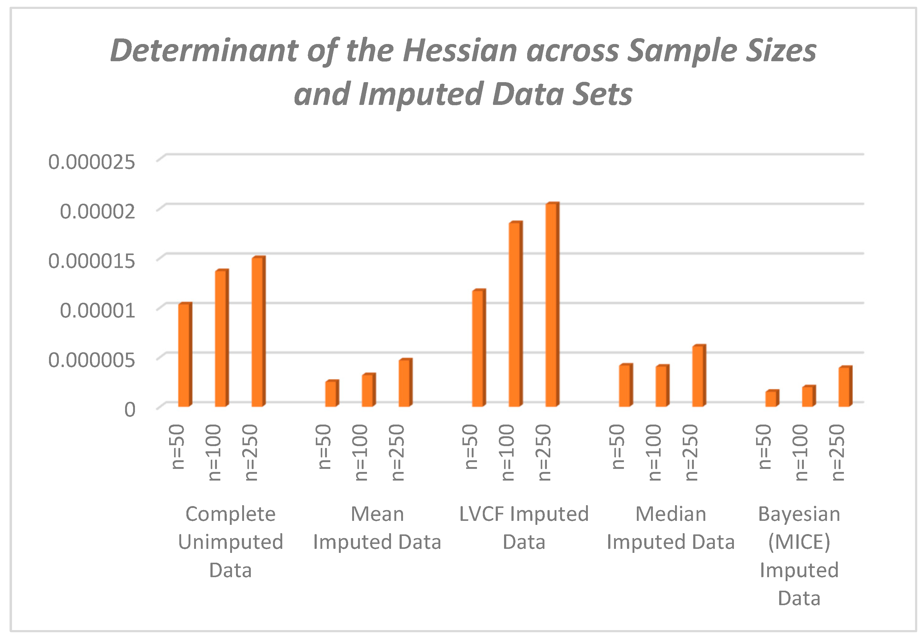
For each data set specified, we find the determinants of the Hessian matrices and plot against the corresponding data code for ease of comparison across sample sizes. We use the determinant of the Hessian matrix as a generalization of the second derivative test for single variable functions. As such if the determinant of the Hessian is positive we have an optimum or extreme value – a maximum if the matrix is negative (semi) – definite. This shows that the log likelihood is a concave function. The imputation techniques used herein are: mean imputation; median imputation; last value carried forward; multiple imputation with chained equations and Bayesian imputation.

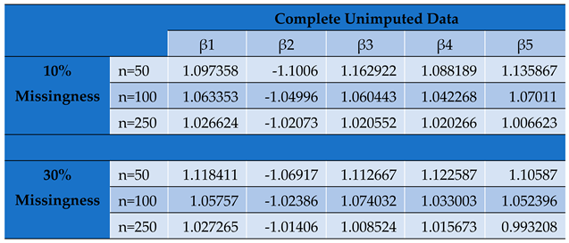
Table 2. Parameter Estimates by Conditional MLE for Complete Unimputed Panel Data Set.

Table 2. Parameter Estimates by Conditional MLE for Complete Unimputed Panel Data Set.

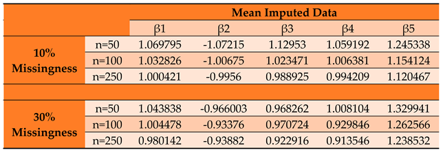
Table 3. Parameter Estimates by Conditional MLE for Mean Imputed Panel Data Set.

Table 3. Parameter Estimates by Conditional MLE for Mean Imputed Panel Data Set.

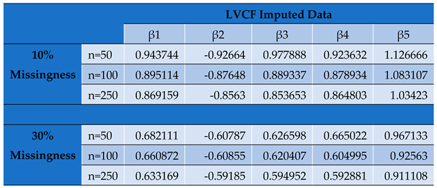
Table 4. Parameter Estimates by Conditional MLE for LVCF Imputed Panel Data Set.

Table 4. Parameter Estimates by Conditional MLE for LVCF Imputed Panel Data Set.

Table 5. Parameter Estimates by Conditional MLE for Median Imputed Panel Data Set.

Table 5. Parameter Estimates by Conditional MLE for Median Imputed Panel Data Set.

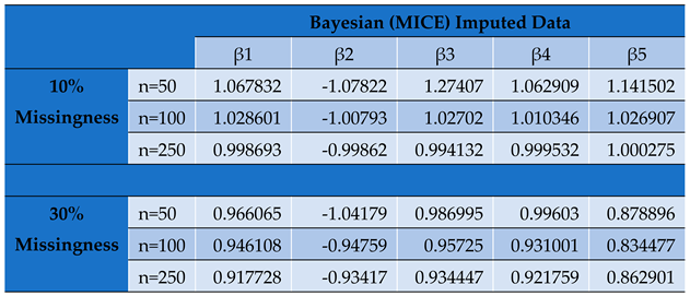
Table 6. Parameter Estimates by Conditional MLE for Bayesian (MICE) Imputed Panel Data Set.

Table 6. Parameter Estimates by Conditional MLE for Bayesian (MICE) Imputed Panel Data Set.

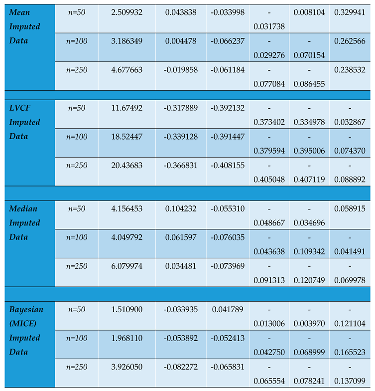
Table 7. Comparative Parameter Biases and Determinants of the Hessian Matrices across Different Imputed Panel Data Sets with Varying sample sizes.

Table 7. Comparative Parameter Biases and Determinants of the Hessian Matrices across Different Imputed Panel Data Sets with Varying sample sizes.

5. Dcussion, Conclusion and Recommendation

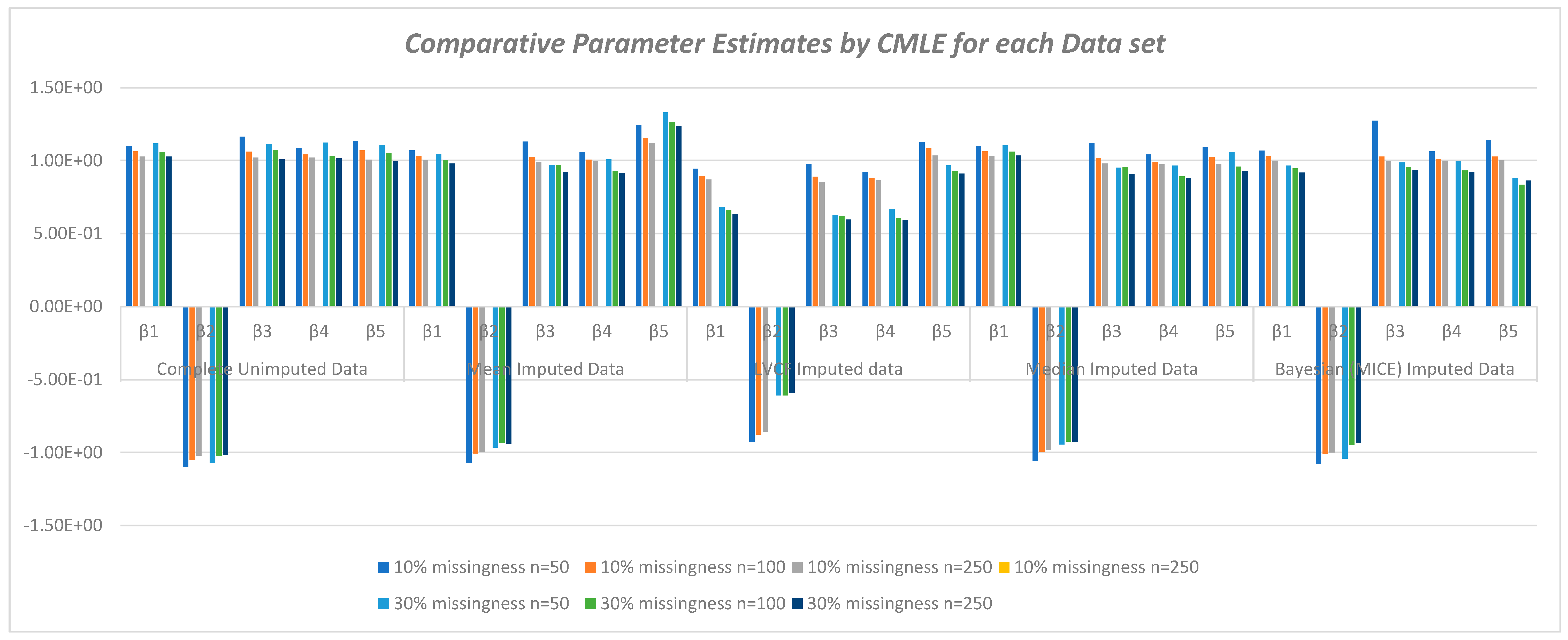
Through the variation of the simulated sample sizes, the study confirms the asymptomatic properties of parameter bias. The results show that the parameter estimates improve with increasing sample size. The precision of the estimates asymptotically increase thereby making them more statistically significant.

The key objectives of this study was to focus on a method used to modify the conditional likelihood function through partitioning of the covariate matrix in a bid to curb the incidental parameter problem and to assess the susceptibility of the Hessian matrix of the log likelihood function on the imputation techniques employed in completing a panel data set with missing covariates.

Undeniably, of all the classical imputation techniques, mean and median imputation do not introduce much undue bias into the data set and therefore perform relatively better than last value carried forward technique and mode imputation. However, model based technique for imputation like MICE yields even better estimates with even more reduced bias and precision [20]. Figure 1 shows the varying and reducing trends of the parameter estimates across sample sizes and across imputation methods used in this study.

The value of $∆{\mathit{x}}_{{\mathit{i}}_{\mathit{I}}}$ impacts inversely on the elements of the Hessian matrix and consequently its determinant. As seen, the study reveals that the smaller the determinant, the larger the parameter estimates which signifies an increased bias for smaller sample sizes. This indicates that by increasing the determinant of the hessian matrix through a reduction in $∆{\mathit{x}}_{{\mathit{i}}_{\mathit{I}}}$values, we reduce the product $\mathit{J}{\left({\mathit{\beta }}^{(h-1)}\right)}^{-1}\mathit{s}\left({\mathit{\beta }}^{(h-1)}\right)$ towards zero.

From the N-R algorithm (30), therefore, the inverse of the Hessian $\mathit{J}$ serves to reduce the product $\mathit{J}{\left({\mathit{\beta }}^{(h-1)}\right)}^{-1}\mathit{s}\left({\mathit{\beta }}^{(h-1)}\right)$ to yield convergence in the iterations of ${\mathit{\beta }}^{\left(h\right)}$. An increasing Hessian modulus therefore ensures faster convergence of the parameter estimates with more precision as seen from table 7 and figure 2. The positive moduli of the Hessian for the conditional MLEs are sufficient for concavity of the log likelihood function that give the optimum estimates of the parameters.

A key importance of deriving the estimators is to increase the theoretical understanding of the estimators and also reduce the computational complexity while estimating logit panel models. As observed from the Monte Carlo results, unbalancedness in a data set biases the parameter estimates and the different imputation techniques employed in this study respond differently to the concavity of the Hessian matrix, hence the bias and efficiency of the estimates are affected too.

Although studies show that the within estimator performs relatively well in many standard situations, this study has demonstrated the advantage of working with the conditional likelihood function over the unconditional likelihood as a working trick to eliminate the fixed effects from the estimation process thereby limiting our concentration on the parameter estimates only.

As a recommendation, further developments can be done on this study by considering multiple fixed effects and observed time periods greater than T=2.

References

- Janssen KJ, Donders ART, Harrell FE Jr., Vergouwe Y, Chen Q, Grobbee DE, Moons KG. Missing covariate data in medical research: to impute is better than to ignore. Journal of Clinical Epidemiology 2010; 63(7):721–727. [CrossRef]
- Donders ART, van der Heijden GJ, Stijnen T, Moons KG. Review: a gentle introduction to imputation of missing values. Journal of Clinical Epidemiology 2006; 59(10):1087–1091. [CrossRef]
- Knol MJ, Janssen KJ, Donders ART, Egberts AC, Heerdink ER, Grobbee DE, Moons KG, Geerlings MI. Unpredictable bias when using the missing indicator method or complete case analysis for missing confounder values: an empirical example. Journal of Clinical Epidemiology 2010; 63(7):728–736. [CrossRef]
- Cox, D.R. and Hinkley, D.V. (1974) Theoretical Statistics. Chapman and Hall, London.
- Firth, D. (1993) Bias Reduction of Maximum Likelihood Estimates. Biometrika, 80, 27-38. [CrossRef]
- Anderson, J.A. and Richardson, C. (1979) Logistic Discrimination and Bias Correction in Maximum Likelihood Estimation. Technometrics, 21, 71-78.
- McCullagh, P. (1986) The Conditional Distribution of Goodness-of-Fit Statistics for Discrete Data. Journal of the American Statistical Association, 81, 104-107. [CrossRef]
- Shenton, L.R. and Bowman, K.O. (1977) Maximum Likelihood Estimation in Small Samples. Griffin’s Statistical Monograph No. 38, London. [CrossRef]
- S. Lee, “Detecting differential item functioning using the logistic regression procedure in small samples,” Applied Psychological Measurement, vol. 41, no. 1, pp. 30–43, 2017.
- R. Puhr, G. Heinze, M. Nold et al., “Firth’s logistic regression with rare events: accurate effect estimates and predictions?” Statistics in Medicine, vol. 36, no. 14, pp. 2302–2317, 2017.
- D. Firth, “Bias reduction of maximum likelihood estimates,” Biometrika, vol. 80, no. 1, pp. 27–38, 1993. [CrossRef]
- Chamberlain, G., (1980). Analysis of Covariance with Qualitative Data, Review of Economic Studies 47, 225-238. [CrossRef]
- Matyas, L. and Lovrics, L. (1991). Missing observations and panel data- A Monte-Carlo analysis, Economics Letters 37(1), 39-44. [CrossRef]
- Neyman, J. and Scott, E.L., (1948). Consistent estimation from partially consistent observations. Econometrica 16, 1-32.
- Lancaster, T., (2000). The incidental parameter problem since 1948, Journal of Econometrics, 95, 391–413. [CrossRef]
- Baltagi, B.H. (2001). Econometric Analysis of Panel Data, 2nd edition, New York, John Wiley.
- Hsiao, C., (2003). Analysis of Panel Data, 2nd edition, New York, Cambridge University Press.
- Greene, W., (2004a). The behaviour of the maximum likelihood estimator of limited dependent variable models in the presence of fixed effects. Econometrics Journal 7(1): 98. [CrossRef]
- Opeyo P.O., Olubusoye O.E. and Odongo L.O. (2014), Conditional Maximum Likelihood Estimation for Logit Panel Models with Non-Responses, International Journal of Science and Research, 3(7), 2242-2254.
- Opeyo, P. , Cheng, W. and Xu, Z. (2023) Superiority of Bayesian Imputation to Mice in Logit Panel Data Models. Open Journal of Statistics, 13, 316-358. [CrossRef]