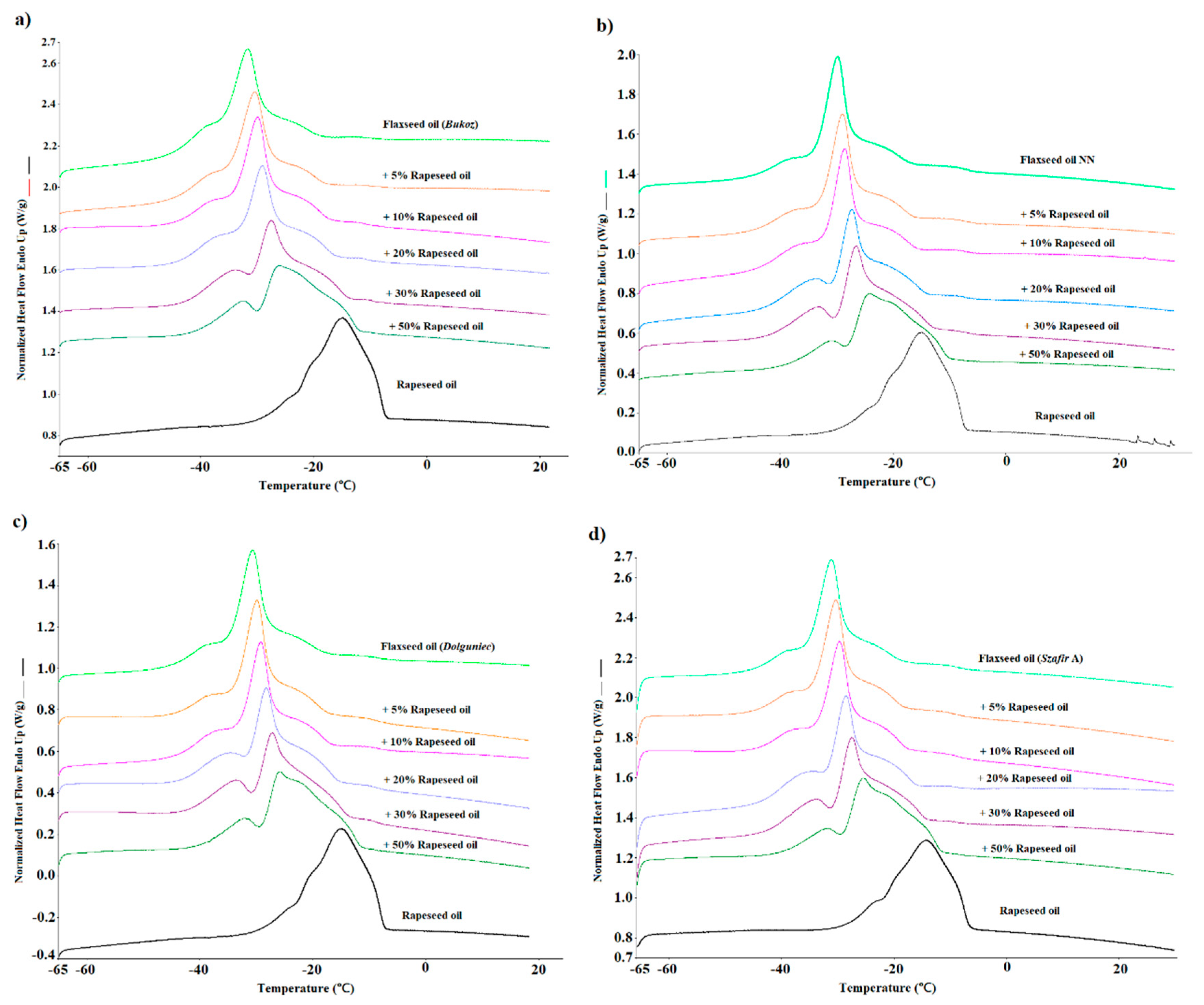
4.1. Classification models for predicting cold-pressed flaxseed oil adulteration levels
In order to assess the ability to build models that classify adulterated oil samples into appropriate classes, the LDA, MARS, SVM and ANNs methods were used. Linear discriminant analysis (LDA) was used to build the first classification model. LDA and the related Fisher's linear discriminant (FLD) are used in machine learning to find the linear combination of features that best distinguish between two or more classes of objects. The resulting combinations are used as a linear classifier. Discriminant analysis resulted in a statistically significant model with Wilks' Lambda = 0.00119 and
p ≤ 0.05. All variables (DSC parameters) except h3 have significant statistical discriminant power. From our study, five discrimination function were obtained based on Wilk’s Lambda statistics, with
p ≤ 0.05 for the first three functions. For purposes of classifying the cases, six classification functions were calculated. Each classification function represents a linear equation that combines the input variables (DSC parameters) to discriminate between six groups (G_1 to G_6) and thus provides different classes (C1 to C6). The case is classified by evaluating the values of the classification functions for that case and assigning it to the class associated with the highest C value. The six classification functions are as following:
Where, variables (i.e., T1, T2, T3, h1, h2, h3, P1, P2 and P3) are DSC parameters related to the case being classified, the constants (e.g., –71.3, –48.9, –127.8, etc.) are regression coefficients (slope), the constant term (e.g., –13488.8, –13326.2, etc.) represents the intercept in the linear equation.
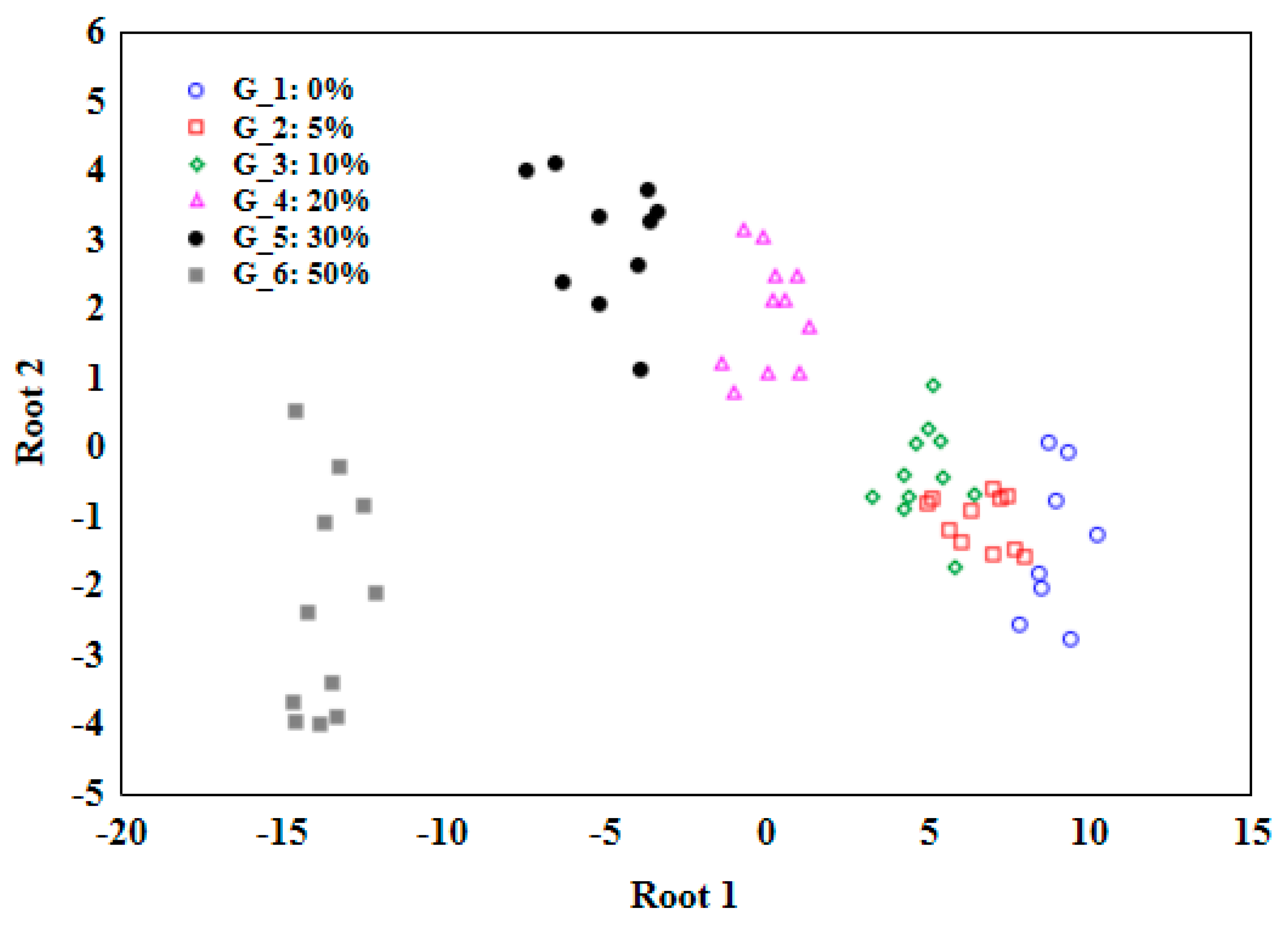
Figure 3 presents the results of the discriminant analysis. From each classification function, a (C) value can be calculated based on the linear combination of the DSC variables and their corresponding coefficients. The higher the C value, the more likely the case belongs to the corresponding class. It's important to note that the coefficients in the classification functions are obtained through the LDA algorithm, which allowed the separation between classes to be maximized, based on the available data from DSC melting curves. The confusion matrix indicated (
Table 2) that only one oil sample with 5% adulteration was classified as a 10% adulterated sample. Thus, the accuracy of the LDA model was 99.5%. A similar approach to detecting adulterations in peanut oil was adopted by other authors, where the identification accuracy was 97% [
14].
MARS regression was used to build the second classification model. Multivariate Adaptive Regression Splines (MAR Splines) is the implementation of a generalization of a technique introduced into wide use by Friedman [
50] and used to solve both regression and classification problems. MARS is a non-parametric procedure requiring no assumptions about the functional relationship between the dependent and independent variables. MAR Splines models this relationship with a set of coefficients and so-called basis functions that are entirely determined from the data. In this study, MARS models created for the data matrix included a maximum of 21 basis functions. The penalty was set to 2, and the threshold to 0.0005. The MARS model of the first order was created for classification purposes and the maximum number of terms was limited by pruning. The model has 6 basis functions and 7 terms with GCV=0.516. Increased numbers of basis functions did not decrease the GCV error. MARS model coefficients and knots are presented in
Table 4. The model developed here allows 90.3% correct classifications to be obtained. The confusion matrix indicated that six samples were incorrectly classified. Therefore, the accuracy of the model based on MARS analysis was about 95.7%, as presented in
Table 3. The MARS regression model was also used by other researchers to define the discriminant surface for studying the authentication of cod liver oil [
15].
Another model which was examined for its usefulness in classifying oil samples into different adulteration classes was the Support Vector Machines (SVM) model. SVM is a method for classifying samples on the basis of the variables (predictors) that describe them. It is a supervised technique, that is, with a supervisor, i.e., there are both variables describing the samples and their membership in defined classes in the learning sample. The support vector method performs classification tasks by constructing hyperplanes in a multidimensional space that separates samples belonging to different classes. For SVM model calculations, the datasets were divided into three subsets in a ratio of 2:1:1 (training, validation, and test set). Samples were classified by the C-SVM method with a linear Kernel type. As a result of learning, a model was obtained that allowed an almost 92% (
Table 2) correct classification of oil samples with 97.3% accuracy (
Table 3). Another study showed the classification accuracy of SVM as 96.25% while comparing chemometrics and AOCS official methods for predicting the shelf life of edible oil [
51].
The last classification model built was an Artificial Neural Network model (ANN). For calculating ANN model, the datasets were divided into three subsets in a ratio of 2:1:1 (training, validation, and test set). The ANN model was trained using selected parameters from the data set and was subsequently validated using an independent data set. Multilayer feed-forward connected ANN was trained with the Broyden-Fletcher-Goldfarb-Shanno (BFGS) learning algorithm (200 epoch). The search for an appropriate ANN model was done using multilayer perceptron (MLP) and radial basis function (RBF) networks. In total, 20 networks were evaluated and the best five were retained. The neural network consists of an input layer, one hidden layer and one output layer. The network architecture, mainly the size of the hidden layer, was selected empirically, taking into consideration the accuracy of predicting the results. The best five ANN-MLP networks are presented in
Table 5.
In the neural network obtained for oil sample classification, the Linear, Exponential and Tanh functions were used in the hidden layer, while Softmax and Exponential functions were used in the output layer. In the input layer, there are 9 neurons, which are DSC parameters. The number of neurons in hidden layer varies from 4 to 11, while the output layer contains 6 neurons representing each class of oil adulteration. A model consisting of the best five networks was used for oil sample classification. The accuracy of the resulting ANN model is almost 98% (
Table 3) with only 3 samples misclassified (
Table 2). This finding can be compared with the study conducted by Firouz et al. [
52], who employed the classification and quantification of sesame oil adulteration, and acquired 100% accuracy.
On the basis of the models’ performance parameters, it was determined that the best model is the LDA model, with the highest values for accuracy (99.5%) precision (98.4%), sensitivity (98.4%), specificity (99.7%) and F1-score (98.4%), and the lowest value of misclassification rate equal 0.54%. In contrast, the worst one was the MARS model, which had the lowest values for accuracy (95.7%), precision (87%), sensitivity (87%), specificity (97.4%) and F1-score (87%) and the highest value of misclassification rate equal 4.3%. The second-best model was the ANN model and the third was the SVM model. The accuracy of all these models was very high, which suggested its ability to predict adulterated oil samples into appropriate classes.
4.2. Regression models for predicting the concentration of refined rapeseed oil in cold-pressed flaxseed oil
Multiple regression analysis (MLR) was performed to formulate a general linear equation which will fit the variables from DSC melting curves against different concentrations of adulterants. This will provide the possibilities to detect the percentage of adulterants in any sample. The MLR model that was obtained was statistically significant with F (9.52) = 364.57 (p ≤ 0.05), R2=0.9844 and adjusted R²=0.9817. The standard error of estimation was 2.3028.
Table 6 demonstrates the summary of DSC parameters, where (b*) values refer to the standardized regression coefficient, and (b) values refer to the regular regression coefficient. Determining (b*) allowed for a direct comparison of the magnitude and importance of the independent variables, where we can see the highest values are presented for h2, T3 and h3 as –0.32, 0.27 and 0.16, respectively. On the other hand, (b) values signify the slope coefficient associated with an independent variable. It represents the change in the dependent variable for a one-unit change in the corresponding independent variable, while holding all other independent variables constant.
Table 6 shows that the h2 (–65.52) variable has the strongest and negative relationship with the concentration variables, indicating that with a decreased value of h2, the concentration of adulterants increased. On the other hand, h3 and T2 variables consequently increase or decrease linearly with the concentration values of adulterants. Accordingly, a model with statistically significant predictors was built.
Where T3 represents the third strongest significant independent variable (p = 0.000), h2 represents the highest strongest significant independent variable (p = 0.000), and h3 represents the second strongest significant independent variable (p = 0.000).
The goodness of fit of the model to the experimental data and the coefficient of determination R2 and the coded coefficient of determination were 0.978 and 0.977, respectively. Equation no. 7 can be used to estimate the percentage of adulterants (for this study, refined rapeseed oil) in a cold- pressed flaxseed oil sample based on three dependent variables: T3, h2, and h3. The equation implies that the variables T3, h2, and h3 are assumed to have a linear relationship with the percentage of the adulterant. The correlation between observed and predicted values was 0.992 with a low RMSE value of 2.12 (
Table 7). A similar study by Sim et al. [
12] showed that it was possible to predict adulteration of lard in palm oil olein using the MLR model, where the prediction performance was measured based on the percentage root mean square error (%RMSE).
MARS regression was used to build the second regression model. In this study, MARS models created for the data matrix included a maximum of 21 basis functions. The penalty was set to 2, and the threshold to 0.0005. The MARS model of the first order was created for classification purposes and the maximum number of terms was limited by pruning. The model has 10 basis functions and 11 terms with GCV=6.252. Equation 8 represents the MARS model for predicting the concentration of refined oil in the samples.
The correlation between the observed and predicted value was 0.995 with a low RMSE value of 1.65 (
Table 7).
Another model which was examined for its usefulness in predicting oil sample adulteration was the Support Vector Machines (SVM) model. SVM can be used for both classification and regression problems. In SVM regression, the search is for a functional dependence of the dependent variable y (% of adulteration) on a set of independent variables x (DSC parameters). For calculating the SVM model, the datasets were divided into three subsets in a ratio of 2:1:1 (training, validation, and test set) for model regression type 1 (C=10.000000, epsilon=0.100000) with radial basis function (gamma=0.111111) kernel type. Samples were classified by C-SVM method with linear kernel type. The correlation between the observed and predicted values was 0.992 with a low RMSE value of 2.1 (
Table 7).
The last regression model built was an Artificial Neural Network model (ANN). For calculating the ANN model, the datasets were divided into three subsets in a ratio of 2:1:1 (training, validation, and test set). The ANN was trained using selected parameters from the data set and was subsequently validated using an independent data set. Multilayer feed-forward connected ANN was trained with the Broyden-Fletcher-Goldfarb-Shanno (BFGS) learning algorithm (200 epoch). The search for an appropriate ANN model was performed using multilayer perceptron (MLP) and radial basis function (RBF) networks. In total, 20 networks were evaluated and the five best were retained. The neural network consists of an input layer, one hidden layer and one output layer. The network architecture, mainly the size of the hidden layer, was selected empirically, taking into consideration the accuracy of the results prediction. The five best ANN-MLP networks are presented in
Table 8.
In the neural network obtained for predicting oil adulteration, the Logistic and Tanh functions were used in the hidden layer, while Logistic, Tanh and Exponential functions were used in the output layer. In the input layer, there are 9 neurons, which are DSC parameters. The number of neurons in the hidden layer varies from 9 to 13, while the output layer contains 14 neurons representing the refined oil concentration. A model consisting of the best five networks was used for prediction purposes. The correlation between the observed and predicted values was 0.996 with a low RMSE value of 1.51(
Table 7). The study found that ANN regression analysis demonstrated robust models for adulteration phenomena in sesame oil generated by sunflower oil, canola oil and sunflower + canola oils quantitatively [
52]. Another study stated that using ANN as a pattern recognition technique for the data obtained from electronic nose could not detect the proportion of adulteration in camellia seed oil, but successfully quantified adulteration in sesame oil [
53].
Table 7 presents the goodness of fit parameters of the regression models obtained. The best model is based on ANN algorithms and exhibits the highest R (0.996), R2 (0.992), adjusted R2 (0.922) values with the lowest values of AIC (233), BIC (240) and RMSE (1.51). The MARS model was next, followed by the SVM, and the least fitting was the MLR model.
4.2.1. Principle component analysis (PCA) and Orthogonal partial least squares discriminant analysis (OPLS-DA)
This adulteration detection study involves analyzing multiple variables of DSC parameters simultaneously. Chemometric techniques like PCA and OPLS-DA are designed to handle multivariate data, allowing for a comprehensive analysis of the oil samples. For instance, PCA presented in
Figure 4 (a) reduced the dimensionality of the dataset by transforming the variables into a smaller set of principal components, capturing the most important variations in the data. Hence, as an unsupervised method, PCA represents the combinations of the original variables and can be difficult to interpret in the context of class separation. To solve this issue, OPLS-DA analysis was adopted for assessing the discrimination and classification of the adulterated flaxseed oil samples. As a fast and efficient screening tool for large datasets, OPLS-DA allowed us to evaluate the effectiveness of DSC melting profiles of adulterated flaxseed oils in classifying and detecting the percentage of adulterants concentration by differentiating them (
Figure 4 b.).
In
Figure 4 (a), DSC data matrix serves as the basis for conducting PCA analyses, which provided a visual representation of the data pattern for six concentrations of adulterants mixed with pure flaxseed oils. In the score plot, each point represents a sample (a specific concentration of adulterant mixed with flaxseed oil) in the space of two principal components, t[
1] and t[
2], which were able to explain 91.1% of the variation of the normalized heat flow results. Additionally, R
2X(cum) and Q
2 (cum) values (
Table 9) are the quantities useful for PC model diagnostics as the fraction of the explained variation R
2X and the fraction of predicted variation Q
2. The more significant a principal component, the closer its R
2X and R
2X (cum) will be to value 1 for a PC model with a sufficient number of components. For the PCA analysis presented in
Figure 4 (a), the R
2X (cum) value was 0.973, which indicates that the retained principal components capture a larger proportion of the overall variation in the dataset. This finding can help in determining the appropriate number of components to retain for further analysis. Besides this, the Q
2 (cum) value was 0.897 for the PCA model, which shows that the cumulative sum of the cross-validated predictive ability is high for the variables of the normalized heat flow of phase transition curves. This approach of employing PCA analysis can be compared to other studies, where researchers detected (with 100% accuracy) adulteration of flaxseed oil with rapeseed, corn, peanut, sunflower seed, soybean, and sesame oils [
25], or adulteration of virgin coconut oil with refined coconut oil [
16].
The next chemometric approach was analyzing the dataset of multiple variables using OPLS-DA, which can effectively enhance the separation of classes while maintaining the predictive power of the model by utilizing orthogonal projection in the score plot. The analysis aims to classify and distinguish different concentrations of adulterants (ranging from 0% to 50%) added to pure flaxseed oil. The model consists of 15 variables, where a total of 9 DSC parameters are considered as X variables and 6 different concentrations of adulterants added are considered as Y variables representing the 6 classes. Five predictive components (P1 to P5) capture the between-class variation, meaning they account for the differences between the different concentrations of adulterants. The orthogonal components capture the within-class variation, representing similarities within each concentration group. Within the framework of the OPLS-DA model, the systematic variation in data was described by two distinct components. The first component, known as the predictive component, exhibits a linear relationship with the classes (Y) and possesses the ability to make accurate predictions. In
Figure 4 (b), the X-axis represents the first component (t1=72.3%) and the Y-axis the second principal component [t2=11.4%]. The observations in the scatter plot are colored, based on their class, which corresponds to the different concentrations of adulterants added to pure flaxseed oil. The scatter plot serves as a visualization of how the modeled observations in the X space are positioned relative to each other. Observations that are close to each other in the plot indicate a higher degree of similarity compared to those that are farther apart.
Also, in
Table 9, the R
2X (cum) value was presented as 0.986, indicating that the OPLS-DA model fits the X data well, capturing a large portion of the variation present in the DSC parameters. On the other hand, a Q
2 (cum) value of 0.33 indicates that the OPLS-DA model can predict approximately 33% of the variation in the Y data, according to cross-validation. The range of Q
2 values suggests that the model has reasonable predictive ability for the concentration of adulterants based on DSC variables. OPLS-DA was also adopted by other authors to determine important variables when detecting flaxseed oil multiple adulteration by near-infrared spectroscopy. These authors also adopted the one-class partial least squares (OCPLS) method to build a detection model which provided a high accuracy of 95.8% [
17].
Although the model demonstrates a good fit to the X data (DSC parameters), a low Q
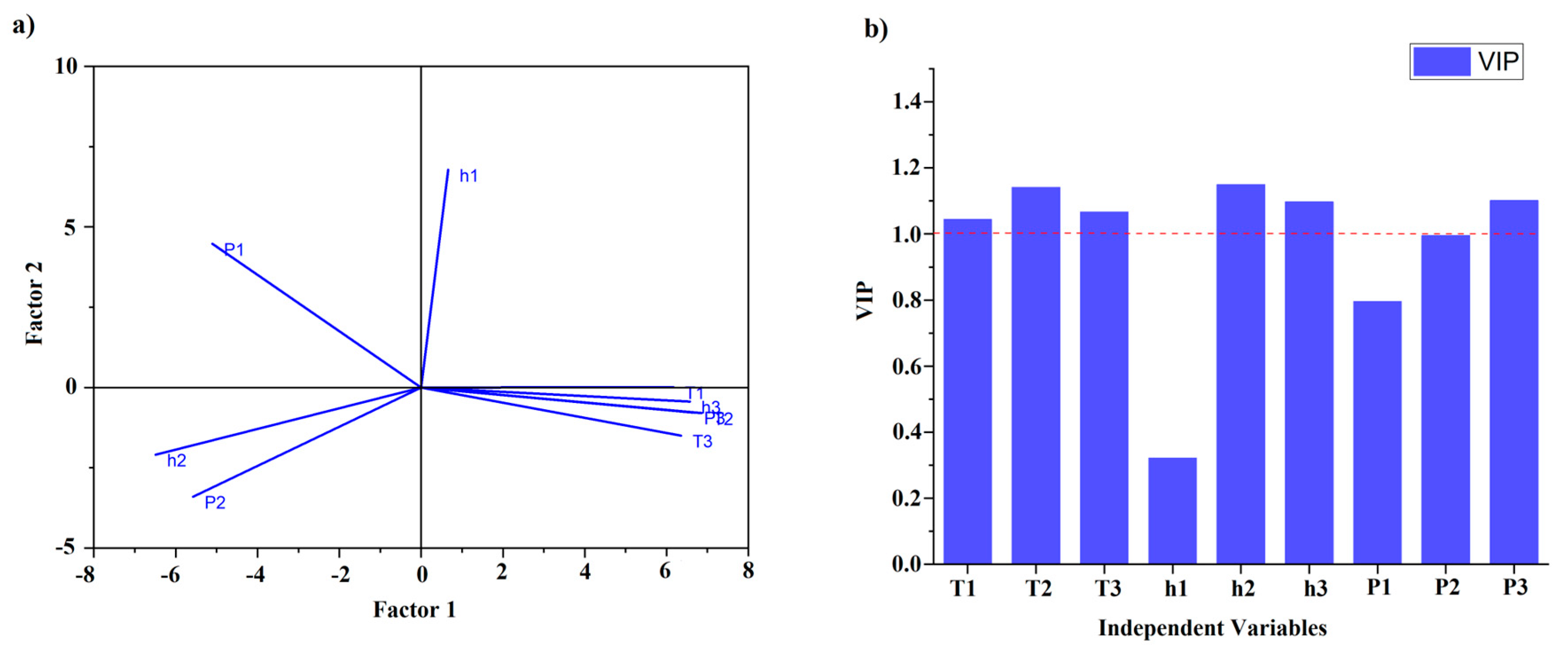
2 (cum) value (0.33) indicates that the model's ability to explain and predict the variation for the Y data (adulterant concentrations) was poor. Thus, the authors decided to explore an alternative modeling technique i.e., the Partial Least Squares (PLS) technique. In
Figure 5 (a), a loading plot of PLS analysis is presented for DSC parameters obtained from the melting curves. To obtain a comprehensive understanding of the model's performance and predictive ability, the R
2X (cum) value was calculated at a level of 0.953 and was lower than for OPLS-DA, while the predictive Q
2 (cum) value was higher than for OPLS-DA (0.973). The results obtained for R2X (cum) and Q
2 (cum) indicate that the PLS model had higher predictive power than OPLS-DA. Additionally,
Figure 5 (b) presents the variables’ influence on the projection (VIP) plot, which provides information about the importance of variables (DSC parameters) which are above value 1. As was the case with the MLR model (
Table 6), the parameter for the first peak height (h1) and percentage area (P1) were not significant.
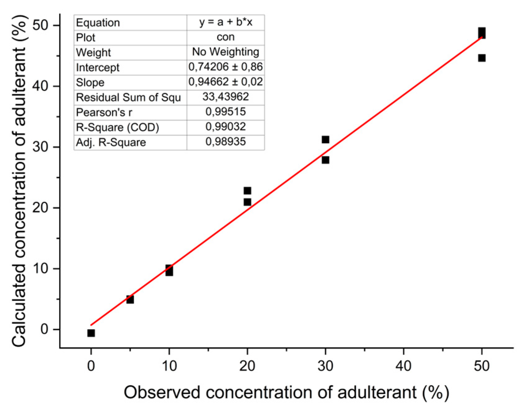
In addition to the approaches presented in the study, the observed and predicted value graph from the PLS model is presented in
Figure 6. By plotting the observed concentrations of adulterants (actual values) against the predicted concentrations (values predicted by the PLS model) on a graph, it was possible to assess visually how well the model predicts the adulterant levels in the flaxseed oil samples, based on the DSC parameters from melting curves. We can see that the observed and predicted values align closely along a diagonal line, which indicates that the PLS model accurately predicts the adulterant concentrations based on the DSC parameters. A Pearson's correlation coefficient (r) of 0.995 between the observed and predicted values indicates an extremely strong positive linear relationship between the two sets of values. This graph also shows that this model can effectively differentiate between pure flaxseed oil and adulterated samples, providing a reliable means of detecting and estimating the adulterant concentrations. By assessing this graph, it is also evident that the PLS model has successfully learned the relationship between the DSC parameters and the adulterant concentrations, which validates the model for this purpose. This finding can be compared with the study conducted by Rocha et al., who adopted the PLS method for the classification and quantification of different types of blended biodiesel synthesized from peanut, corn, and canola oils, and observed a Pearson's correlation coefficient of 0.969 between the real and predicted concentrations [
13].


