1. Introduction
The coronavirus infection is a highly contagious viral disease that has effect and spread to almost every country in the world. It is caused by a virus called Severe Acute Respiratory Syndrome coronavirus 2 (SARS-CoV-2) and that was firstly identified in December 2019. In March 2020, the World Health Organization (WHO) declared COVID-19 a pandemic due to its rapid spread and impact on millions of people worldwide [
1]. After certain time period COVID-19 has affected more people than previous outbreaks of MERS and SARS. The initial outbreak of COVID-19 cases was detected in Wuhan, China. Many individuals infected with proposed virus may not show any symptoms or only experience mild symptoms. However, those with symptoms typically experience a muscle or joint pain, dry cough, fever and in many active cases, specially shortness of breath which was more painful stage for effected people. COVID-19 poses a significant risk to individuals with pre-existing health conditions such as diabetes, kidney disease, cardiovascular and obesity disease. Most of the people with chronic respiratory diseases are especially vulnerable to severe complications and death from COVID-19. The primary mode of transmission is through direct contact with attenuated objects or surfaces, as well as consumption of respiratory aerosol from infected individuals, whether they show symptoms or not [
2].
The COVID-19 pandemic continuously to show mannerism a significant threat to people worldwide, particularly due to the increasing incidence of infection in certain countries. Consequently, it has become crucial to detect, assess, and understand the exempt feedback to SARS-CoV-2 disease. While diseases like Polio can be controlled by regular vaccination to the children below a certain 5 years of age and most of medicines and antibiotics can help to manage the outbreaks of infection, some infectious diseases such as TB, Cholera, and Malaria still cause fatalities globally [
3]. However, recently some effective and safe vaccines have been developed by many countries still rely on non pharmaceutical mediation like social distancing, lock downs, and face masks to contest the infection. Nonetheless, vaccination remains an effective and simple strategy in controlling infectious diseases, as demonstrated by the successful eradication of smallpox through vaccination [
4]. Consequently, scientists worldwide are agreeing in development of effective COVID-19 vaccines, recognizing their potential to safe countless lives as a new tool in the battle against the virus [
4].
In order to gain a deeper comprehension of how epidemic illnesses work and suggest more effective approaches to prevent their spread, mathematical models can be highly valuable. These models serve as helpful tools for predicting the patterns and progression of diseases, allowing us to implement strategies that can reduce the rate of infection and mortality. Recent advancements have introduced new mathematical models specifically designed to forecast disease dynamics and flatten the curves of infection and death [
5,
6]. Moreover, numerous compartmental mathematical models have been developed to explore the influence and significance of vaccination in combating various infectious diseases, as detailed in a range of studies [
7,
8,
9,
10].
Based on the existing literature, the focus of this study is to develop a new stochastic model that can analyzed the dynamics of COVID-19, taking into account the impact of vaccination. The proposed model incorporates a stochastic term to enhance its accuracy. The first objective of current research is to examine the transmission patterns of COVID-19, specifically in relation to Non-Pharmaceutical Interventions (NPIs) and the vaccination process. To establish the parameters of the model, actual pandemic cases in Pakistan are used for estimation. The study also presents the basic reproduction number and equilibrium points, along with conducting various fundamental analysis. The research findings from this study can be valuable for government authorities and public health agencies in formulating effective strategies to minimize the spread of future outbreaks.
This research paper is organized into different sections to provide a comprehensive analysis of the stochastic COVID-19 vaccination model. In
Section 2, we present the mathematical modeling of this model, which involves describing the various factors and variables that influence the spread of the virus and the effectiveness of vaccinations. To further enhance our understanding,
Section 3 reviews the application of Legendre polynomials and the spectral method in this context, as these mathematical tools have proven valuable in analyzing complex systems. In
Section 4, we briefly discuss the basic reproduction number, an important metric in epidemiology, and conduct a stability analysis to assess the robustness of our model. In
Section 5, we delve into the numerical results obtained from our simulations and discuss their implications for COVID-19 vaccination strategies. Finally, we conclude our research paper by summarizing our findings and highlighting the key takeaways in the last section.
2. Stochastic COVID-19 vaccine model
In this section, we focus on modeling a stochastic COVID-19 vaccination model to investigate the impact of certain non-pharmaceutical interventions (NPIs), specifically social distancing in combination with vaccination. Although the COVID-19 vaccine is currently in an experimental phase and only available to a limited extent, it plays a crucial role in controlling the pandemic alongside other pharmaceutical mediation. To construct mathematical model, we divide the total population into distinct classes: susceptible individuals (S(t)), vaccinated individuals (V(t)), exposed individuals (E(t)), asymptomatic infected individuals (), the symptomatic infected individuals (I(t)) and recovered from infection is denoted by (R(t)). Where, total population (N(t)) is the sum of all above classes.
The proposed model for the stochastic COVID-19 vaccine can be represented as a set of stochastic differential equations, which are nonlinear in nature. Mathematically, this model describes the relationship between various factors involved in the vaccine’s effectiveness and its impact on the spread of the disease. By using these equations, we can better understand and predict how the vaccine will interact with the virus and the human immune system, providing valuable insights into its potential efficacy.
with positive initial values
, respectively for each class.
In the considered system described by Eqs.
1, the parameter
represents the assumed birth rate, whereas
denotes the natural death rate within each class of the model. The rate at which susceptible individuals receive vaccinations is represented by
, and those who have been vaccinated become susceptible again at a rate of
. Latent individuals become infected at a rate of
, where the remaining individuals (proportion
r) join the group of asymptomatic infection. Where parameter
shows the COVID-19 convinced mortality rate, while
and
indicate the rate at which both symptomatically and asymptomatically infected individuals recover. The transmission of the disease is characterized by
, and the transmissibility coefficient of asymptomatic individuals is denoted by
.
It is expected that all the parameters have positive values.
In present research work, we implement the spectral method for the numerical solution of COVID-19 system. This method were initially applied for differential and integral system [
11,
12,
13]. Moreover, for numerical solutions of different diseases models the proposed method are applied by authors [
14,
15,
16,
17].
Since infectious diseases are subject to randomness in terms of the nature of transmission, the deterministic COVID-19 model given in Eqs.
1 is perturbed by white noise to obtain a stochastic model given in form:
In this study, we are focusing on the spectral method for obtaining the solution to a stochastic COVID-19 model described by Eqs.
2. In this model,
represents Brownian motion, which is a random process that exhibits erratic behavior over time. The parameter
is referred the intensity of Brownian motion, which determines the degree of randomness or volatility in the system. By developing an approximate solution to this stochastic model, we aim to better understand and predict the dynamics of COVID-19.
3. Spectral Method
Before apply spectral method, to provide an preview of Legendre polynomials given in [
18]. The
order Legendre polynomials denoted by
. Where the function
is approximated by:
indicates Legendre coefficients,
are collocation nodes and
denotes
-order. Where the Legendre polynomials are:
Spectral method procedure we considered the Legendre-Gauss-Lobatto points .
For this, taking integral on Eq.
2 from
.
where
are initial conditions on the functions of each class respectively. To convert the present interval to
interval, we transform
s like:
, then Eqs.
5 becomes:
where the semi discretized spectral system Eqs.
6 are:
where the weight function refer [
12,
13], for Eq.
1 is given by
L is the Lagrange polynomials.
Also the weight function for Eq.
2 is given by
Now the spectral solution of each
and
R by using the above Eq.
5
Legendre coefficients of each of functions
,
,
,
,
and
are in the form:
, respectively. Now using the solution Eqs.
9 becomes:
We take
. The proposed system Eqs.
9 gives of
of unknowns in which
nonlinear equations. Using initial conditions say:
Eqs.
10 and Eqs.
9 of a system of
equations. Therefore, the solving the above two systems gives the solution of corresponding all unknowns. In last using the unknown values in Eqs.
8, and get a solution to the model given in Eqs.
2.
4. Stability Analysis
Stability analysis is a crucial tool for investigating the behavior of a dynamical system. In this particular section, we delve into the examination of the stability of equilibrium solution. These equilibrium solutions are associated with both deterministic and stochastic systems, which are represented by equations labeled as Eqs.
1 and Eqs.
2 respectively. By studying the stability of these solutions, we gain insights into how the system’s dynamics unfold over time, accounting for both deterministic and random influences.
The COVID-19 model described by Eqs.
1 can have up to two equilibrium solutions. The first one, called the infection-free equilibrium
, represents a steady state solution where there is no disease in the population. The second equilibrium solution is known as the endemic equilibrium, which occurs when the disease persists within the population.
4.1. Basic reproductive number () by Next-generation
matrices method
The system of Eqs.
2 provide the simple vaccination model that describes the coronavirus disease. Now the infectious subsystem of Eqs.
2 gives that,
So the jacobian matrix of the Eqs.
11 is computed as
As seen below, the Jacobi matrix is split into two matrices
And the transition matrix inversion is
By analyzing the following classes instances, the basic reproductive equation (
) may be constructed. Now the NGM with large domain is denoted by
is given by:
In light of this, the basic reproduction formula for a matrix with a large domain is
Following equation gives the reproduction number for the system given by Eqs.
1
Theorem 4.1.
If , then disease-free equilibrium is a stable solution for a system described by equations Eqs. 1 on the entire region , which means that disease will not be spread and the population will remain healthy. On the other hand, if , then the endemic equilibrium solution (with values , , , , , and ) of the system described by equations Eqs. 1 is asymptotically stable on the region . This implies that the disease will persist in the population.
Proof. The endemic equilibrium
of system given by Eq.
1, has stationary system is given by:
To solve system in Eq.
16. We will discuss two major cases:
- a.
infected classes I and equal to zero
- b.
I and greater than zero.
- (a):
If
: then from the last equation of Eqs.
16, we get
, where from equation number four of Eqs.
16, we get
, and using equation first, we get
. Similarly from the fifth equation we get
. Therefore, we get the disease free equilibrium
, having a case
- (b):
If and , for the lake of calculation using Maple-13 software to found the proposed endemic equilibrium In this case should be .
□
Lemma 4.2. Total region say is positive invariance set for the proposed model given in Eqs. 1.
Proof. For
, then using model Eqs.
1, we get:
Therefore, Eq.
18 takes the form:
Hence in the total region
the system Eq.
1 is positively invariant. □
The following lemma are proved by using method refer [
19],.
Lemma 4.3.
The solution of system Eqs. 1 has above properties for each initial condition :
and similarly for each class.
Definition 4.4. Individuals that are infected in population I and are termed extinctive for model Eqs. 2 if and only if .
Theorem 4.5.
Since, or with , then both the infected classes I and of Eq. 2 are exponentially tends to zero. Conversely, if , the each class of the model Eqs. 2 are present, where
Proof. Suppose the solution of the proposed vaccination model Eq. (
2) in the form of
along with initial conditions
. Also assume that
, then by using It
formula we get:
Apply integral from 0 to
t, we have
here we discuss the two cases, if
, then
Divide Eq. (
21) by
, then
By taking
and using Lemma 4.3, then Eq. (
22) converted to
Which shows,
The second case, when
, and using Eq. (
20) we get
Dividing Eqs. (
23) by
t where
we obtain
Again by taking
and use Lemma 4.3, Eq. (
24) becomes
Which shows that
□
5. Numerical Results
Current section focuses on presenting some numerical problems and their corresponding graphical results. The numerical results are captured and explained for both deterministic system Eqs.
1 and the stochastic system Eqs.
2. To find these numerical results, the spectral collocation method is employed. The obtained results are then visualized in
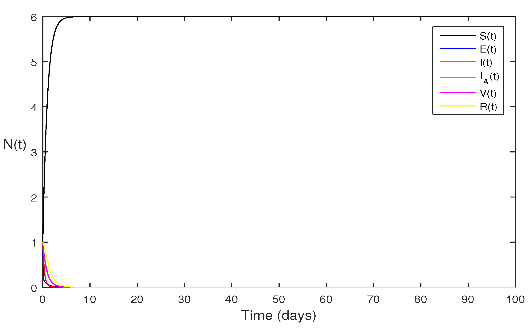
Figure 1,
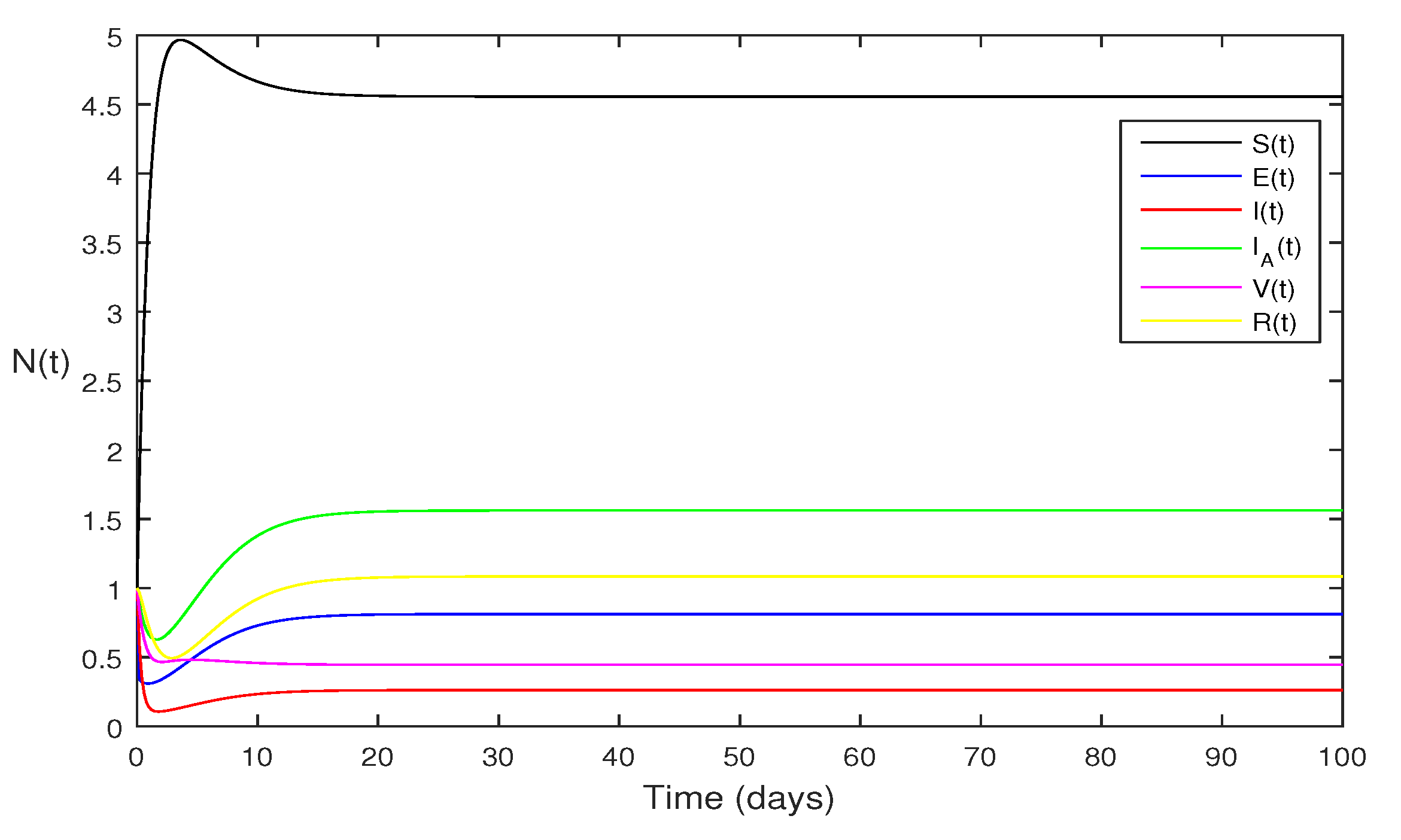
Figure 2,
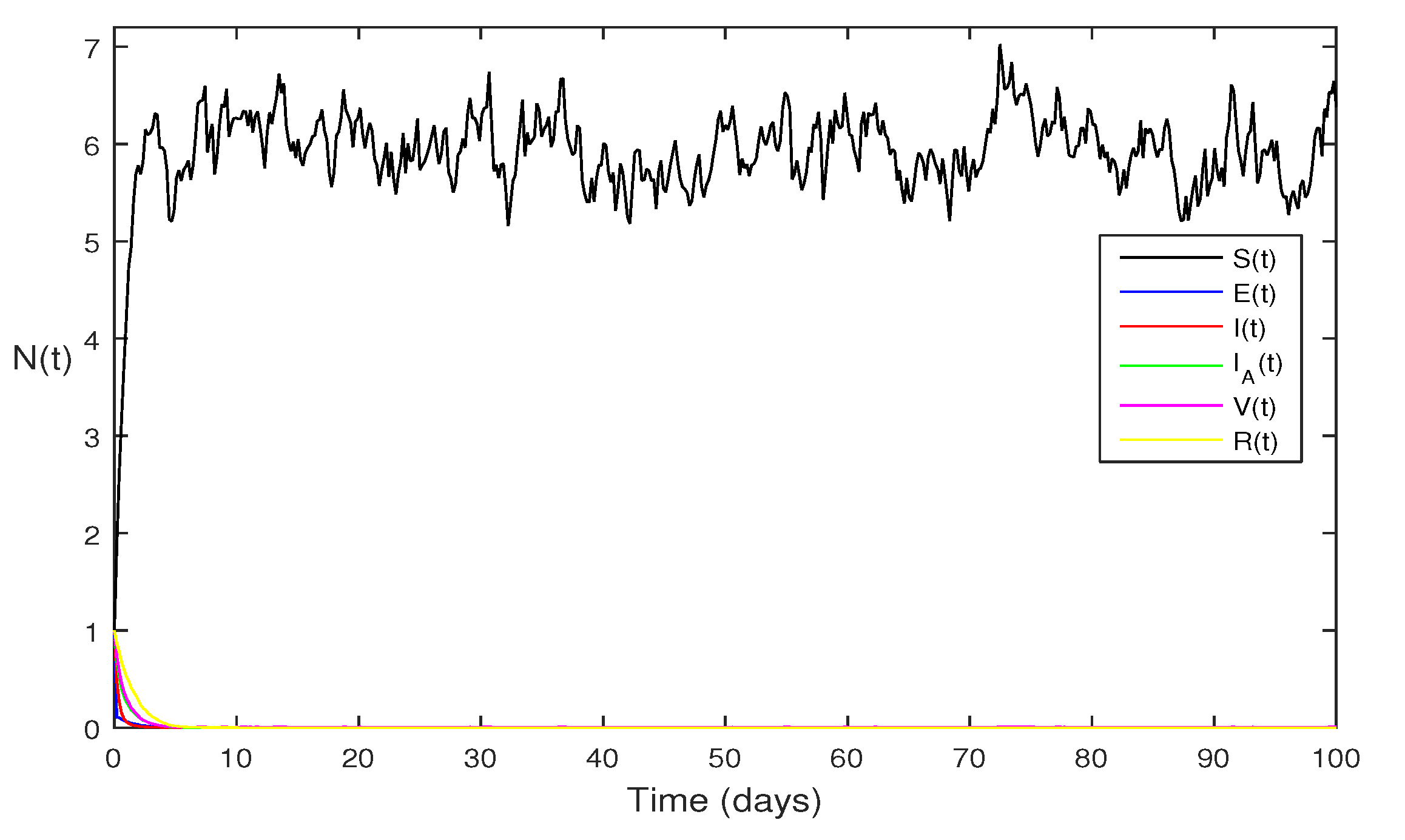
Figure 3,
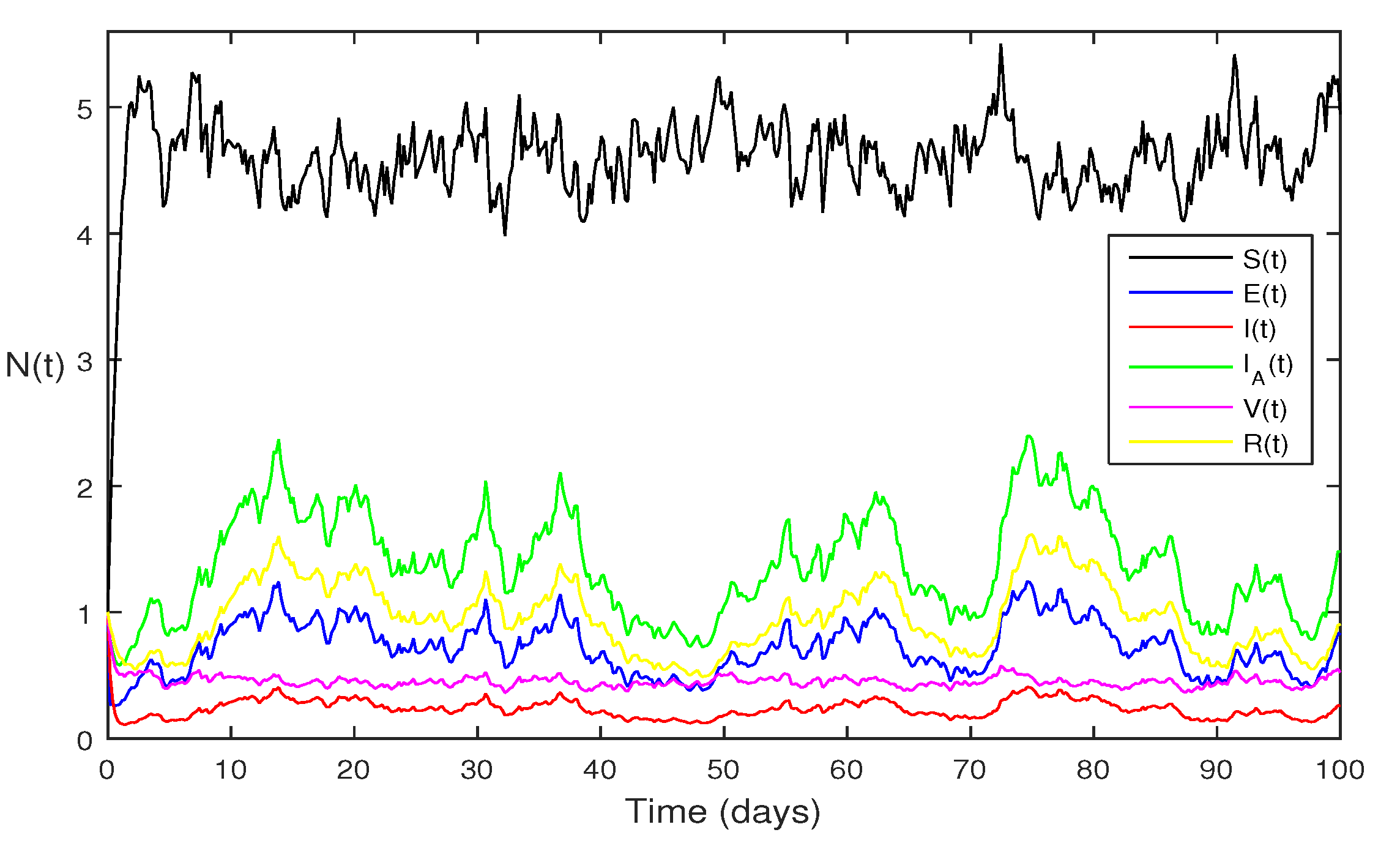
Figure 4,
Figure 5,
Figure 6,
Figure 7,
Figure 8. The computations for this study are performed on a personal computer using Maple and Matlab software. To simplify the calculations, each initial value is assumed to be equal to 1.
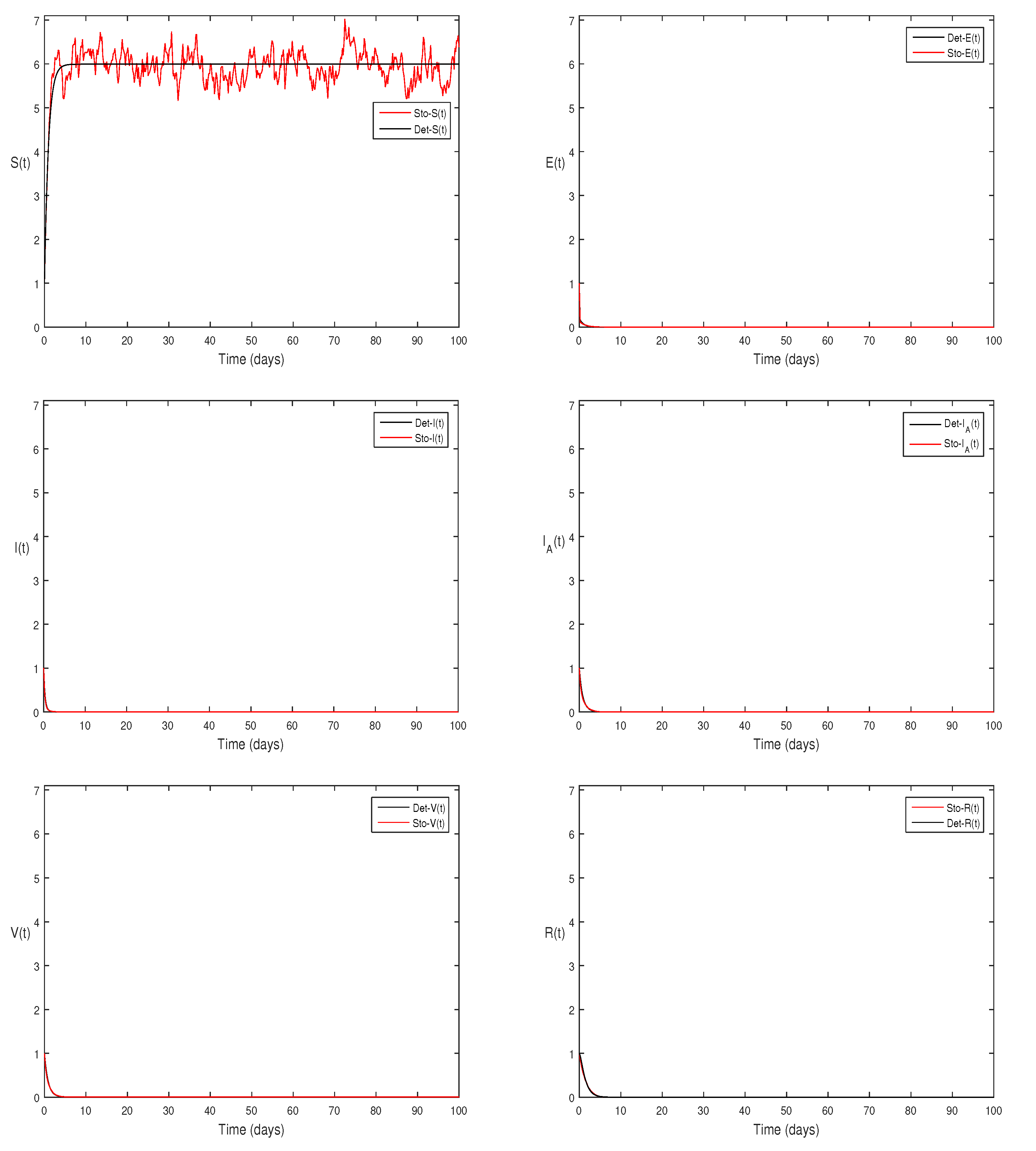
Figure 1 Following parameter values are assumed for deterministic system Eqs.
1 as
. The computations gives reproduction number becomes
, by using given parameter values. By using theorem 4.1, we see the model Eqs.
1 has stable infectious free equilibrium
where
is in the form
.
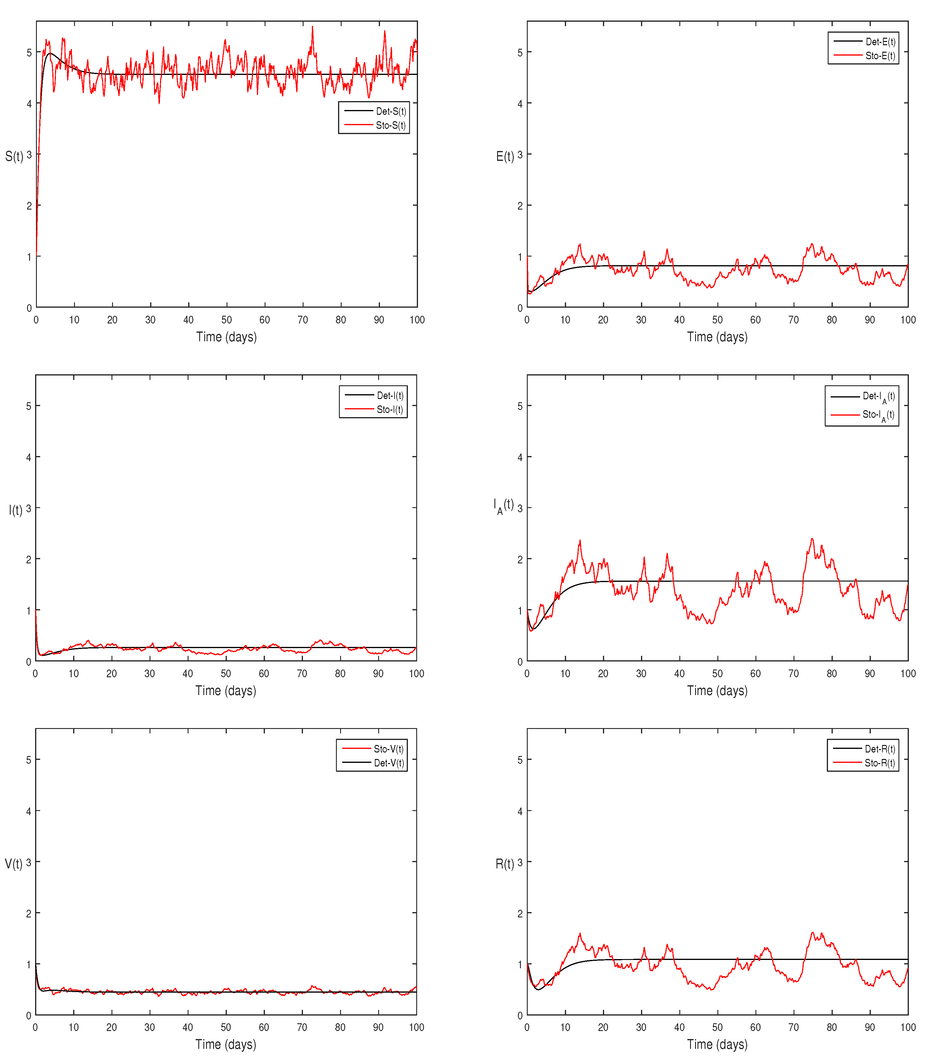
Figure 2 If we change
and
and remaining the same as in
Figure 1. Then we got
and using theorem 4.1 the model Eqs.
1 has stable endemic equilibrium and all the compartments are then zero as given in
Figure 2.
Figure 3 When we chosen parameter values
for stochastic system Eqs.
2. The above simulation shows that
and
along with theorem 4.5 the infected classes of model Eqs.
2 becomes zero.
Figure 4 Choose
and
and remaining the same parameter values of
Figure 3, then the stochastic model Eqs.
2, satisfy
, with
using theorem 4.5, shows that each class are presents of Eqs.
2, this can be performed in
Figure 4.
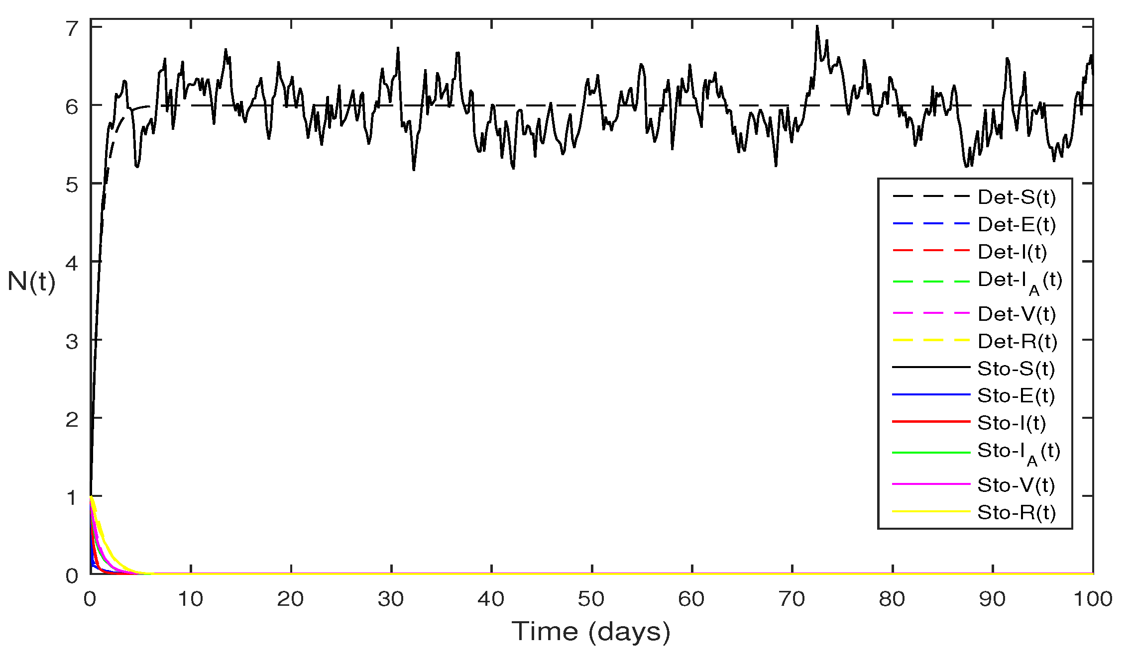
Figure 5 Present figure show the comparison of the solutions Eqs.
1 and Eqs.
2 for each classes, where using parameter values
. The simple computation shows that for model Eqs.
1 , where for stochastic model Eqs.
2 with
Using the theorems 4.1 and 4.5, we see both the systems satisfy the disease free equilibriums.
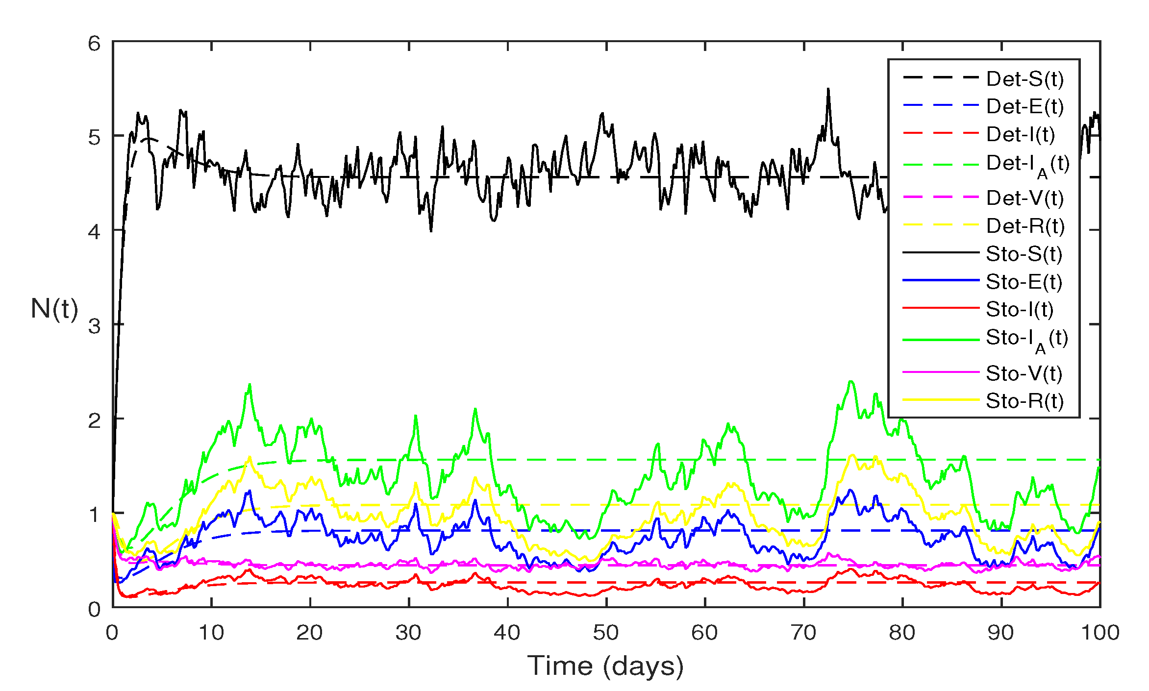
Figure 6 Comparison of both models given in Eqs.
1 and Eqs.
2 for each classes, using following values of parameter
and
and remaining the same parameter values as in
Figure 5. Using such parameter values the Eqs.
1 , also for stochastic model Eqs.
2 with
Using the theorems 4.1 and 4.5, we see both the systems satisfy endemic equilibriums.
Figure 7 Above same parameter values as given in
Figure 5 to compare both the deterministic and stochastic solutions.
Figure 8 The same parameter values as given in
Figure 6 to compare both the deterministic and stochastic solutions.
6. Conclusions
The use of mathematical modeling combined with numerical analysis using spectral techniques has been shown to be a highly effective approach for gaining deeper insights into the transmission dynamics of diseases. This research introduces a new epidemic model that is analyzed rigorously mathematically to investigate the transmission dynamics of the COVID-19 pandemic, taking into account the impact of vaccination. The crucial measure of disease spread, known basic reproduction number, is found using the next-generation method. Stability of the disease-free equilibrium is proven to be asymptotically stable when the basic reproduction number becomes (). On the other hand, the stable endemic equilibrium is established when is greater than 1. To incorporate the effects of vaccination, a vaccination strategy is incorporated into the model. After conducting a various analysis, the proposed models are solved numerically using a highly efficient spectral approach called the high order spectral scheme, which utilizes Legendre collocation nodes. Finally, with the estimated parameter values, the model is simulated to assess the impact of non-pharmaceutical mediation and the effectiveness of vaccination on the transmission dynamics and also to control of the proposed pandemic. In conclusion, the results indicate that by increasing the low transmission rate through preventive calculated like social distancing and following strict SOPs, along with achieving herd immunity through a highly effective vaccine, the pandemic can be effectively curtailed.
Funding
Project number (RSPD2023R576), King Saud University, Riyadh, Saudi Arabia.
Acknowledgments
Researchers Supporting Project number (RSPD2023R576), King Saud University, Riyadh, Saudi Arabia.
Conflicts of Interest
The authors declare no conflict of interest.
References
- Ullah, S.; Khan, M.A.; Farooq, M.; Gul, T. Modeling and analysis of tuberculosis (TB) in Khyber Pakhtunkhwa, Pakistan. Mathematics and Computers in Simulation 2019, 165, 181–199. [Google Scholar] [CrossRef]
- Adams, J.; MacKenzie, M.J.; Amegah, A.K.; Ezeh, A.; Gadanya, M.A.; Omigbodun, A.; Silverman, M. The conundrum of low COVID-19 mortality burden in sub-Saharan Africa: myth or reality. Global Health: Science and Practice 2021, 9, 433. [Google Scholar] [CrossRef] [PubMed]
- Mhlanga, A. Dynamical analysis and control strategies in modelling Ebola virus disease. Advances in Difference Equations 2019, 1–27. [Google Scholar] [CrossRef]
- Bhavya, B.M.; Doddamani, S.H.; Shubhashree, M.N. An Overview on Ayurvedic Remedies in Overcoming Communicable Illnesses and Its Contemporary Relevance WSR COVID-19. Rivista Medicine 2022, 149–152. [Google Scholar]
- Koca, I. Analysis of rubella disease model with non-local and non-singular fractional derivatives. An International Journal of Optimization and Control: Theories and Applications (IJOCTA) 2018, 8, 17–25. [Google Scholar] [CrossRef]
- Upadhyay, R.K.; Roy, P. Spread of a disease and its effect on population dynamics in an eco-epidemiological system. Communications in Nonlinear Science and Numerical Simulation 2014, 19, 4170–4184. [Google Scholar] [CrossRef]
- Cai, L.M.; Li, Z.; Song, X. Global analysis of an epidemic model with vaccination. Journal of Applied Mathematics and Computing 2018, 57, 605–628. [Google Scholar] [CrossRef] [PubMed]
- Li, X.P.; Gul, N.; Khan, M.A.; Bilal, R.; Ali, A.; Alshahrani, M.Y.; Islam, S. A new Hepatitis B model in light of asymptomatic carriers and vaccination study through Atangana-Baleanu derivative. Results in Physics 2021, 29, 104603. [Google Scholar] [CrossRef]
- Sulayman, F.; Abdullah, F.A.; Mohd, M.H. An SVEIRE model of tuberculosis to assess the effect of an imperfect vaccine and other exogenous factors. Mathematics 2021, 9, 327. [Google Scholar] [CrossRef]
- Khan, Muhammad Altaf, et al. Global stability and vaccination of an SEIVR epidemic model with saturated incidence rate. International Journal of Biomathematics 2016, 9, 1650068. [Google Scholar]
- Gul, Naseeb, et al. Transmission dynamic of stochastic hepatitis C model by spectral collocation method. Computer Methods in Biomechanics and Biomedical Engineering 2022, 25, 578–592. [Google Scholar] [CrossRef] [PubMed]
- Ali, Asad, et al. On dynamics of stochastic avian influenza model with asymptomatic carrier using spectral method. Mathematical Methods in the Applied Sciences 2022. [Google Scholar]
- Khan, Sami Ullah and Ali, Ishtiaq. Application of Legendre spectral-collocation method to delay differential and stochastic delay differential equation. AIP Advances 2018, 8, 035301. [Google Scholar] [CrossRef]
- Khan, Sami Ullah and Ali, Mushtaq and Ali, Ishtiaq. A spectral collocation method for stochastic Volterra integro-differential equations and its error analysis. journal Advances in Difference Equations 2019, 1, 161. [Google Scholar]
- Khan, Sami Ullah and Ali, Ishtiaq. Numerical analysis of stochastic SIR model by Legendre spectral collocation method. Advances in Mechanical Engineering 2019, 11. [Google Scholar]
- Ali, Ishtiaq, and Sami Ullah Khan. Analysis of stochastic delayed SIRS model with exponential birth and saturated incidence rate. Chaos, Solitons and Fractals 2020, 138, 110008. [Google Scholar] [CrossRef]
- Khan, Sami Ullah and Ali, Ishtiaq. Convergence and error analysis of a spectral collo- cation method for solving system of nonlinear Fredholm integral equations of second kind. Computational and Applied Mathematics 2019, 38, 125. [Google Scholar] [CrossRef]
- Khan, Sami Ullah, and Ishtiaq Ali. Applications of Legendre spectral collocation method for solving system of time delay differential equations. Advances in Mechanical Engineering 2020, 12, 1687814020922113. [Google Scholar]
- Song, Y.; Miao, A.; Zhang, T.; Wang, X.; Liu, J. Extinction and persistence of a stochastic SIRS epidemic model with saturated incidence rate and transfer from infectious to susceptible. Advances in Difference Eqnarrays 2018, 2018, 293. [Google Scholar] [CrossRef]
|
Disclaimer/Publisher’s Note: The statements, opinions and data contained in all publications are solely those of the individual author(s) and contributor(s) and not of MDPI and/or the editor(s). MDPI and/or the editor(s) disclaim responsibility for any injury to people or property resulting from any ideas, methods, instructions or products referred to in the content. |
© 2023 by the authors. Licensee MDPI, Basel, Switzerland. This article is an open access article distributed under the terms and conditions of the Creative Commons Attribution (CC BY) license (http://creativecommons.org/licenses/by/4.0/).
