Submitted:
27 July 2023
Posted:
28 July 2023
You are already at the latest version
Abstract
Keywords:
1. Introduction
2. Methodology
2.1. Color Data Acquisition Based on Spectral Reconstruction
2.2. Color Fastness Prediction Methods
2.2.1. Existing Methods
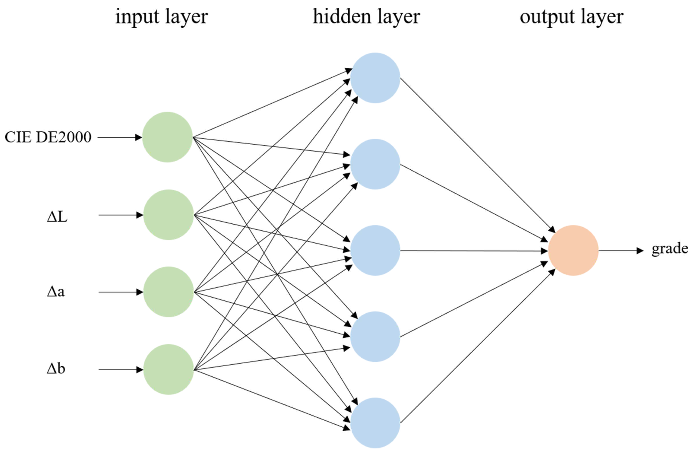
2.2.2. The Proposed Method
2.3. Evaluation Metrics
3. Experiment
3.1. The Rubbing Color Fastness Experiment
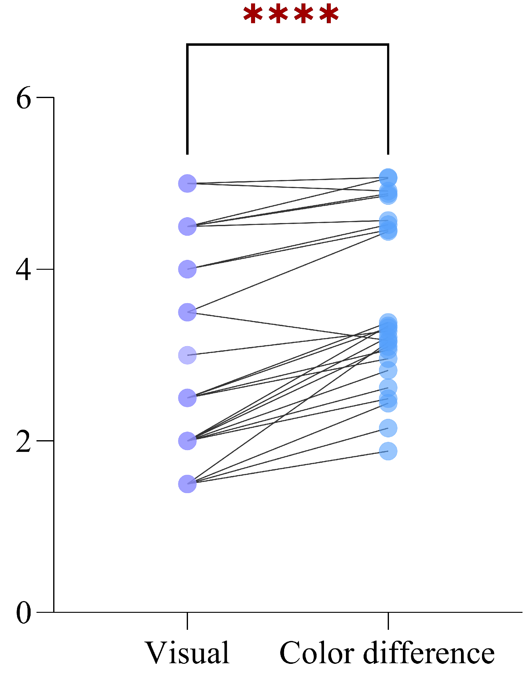
3.2. The Visual Rating Experiment
3.3. The BP Neural Network Modeling
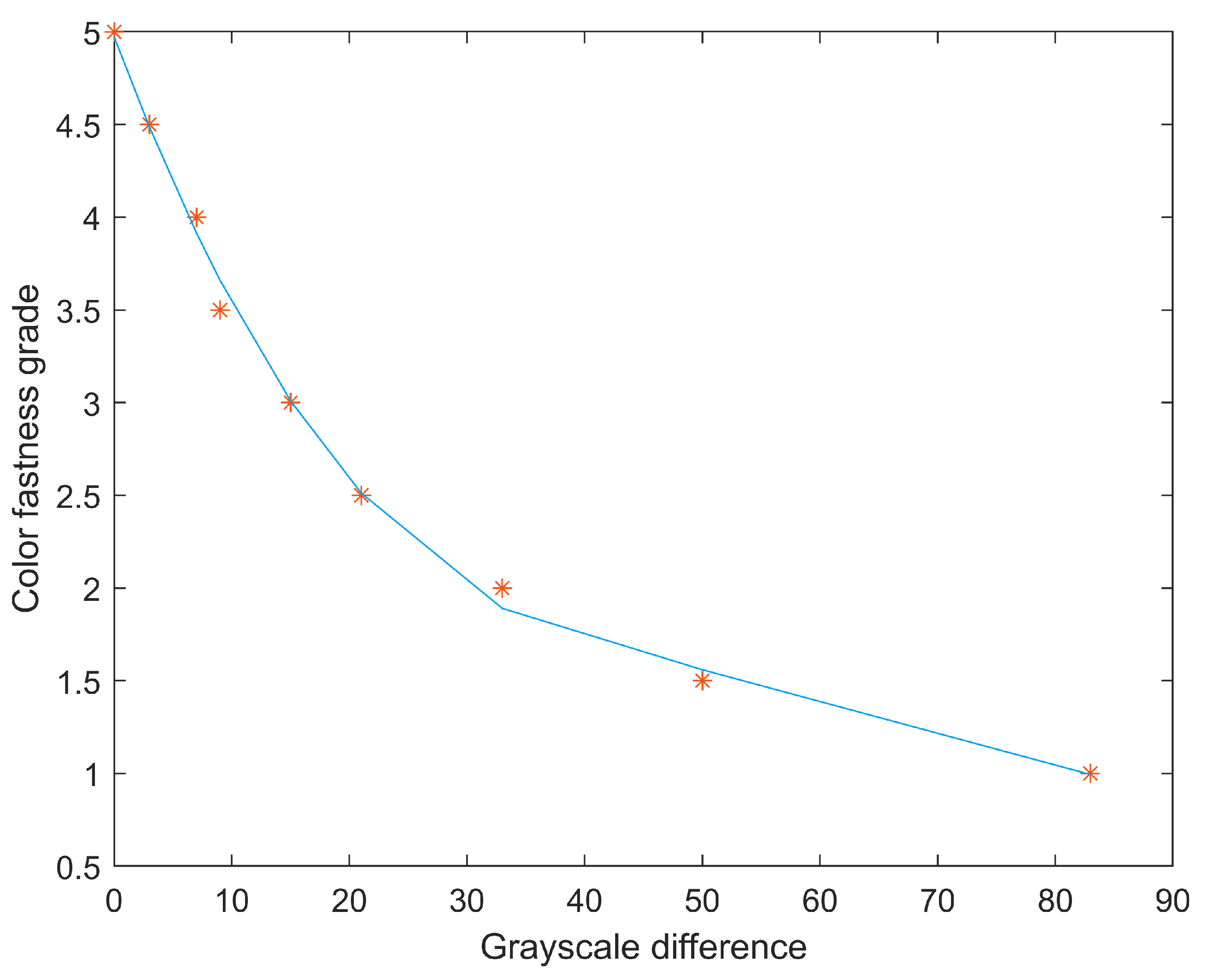
3.4. Testing of Existing Methods
4. Results and Analysis
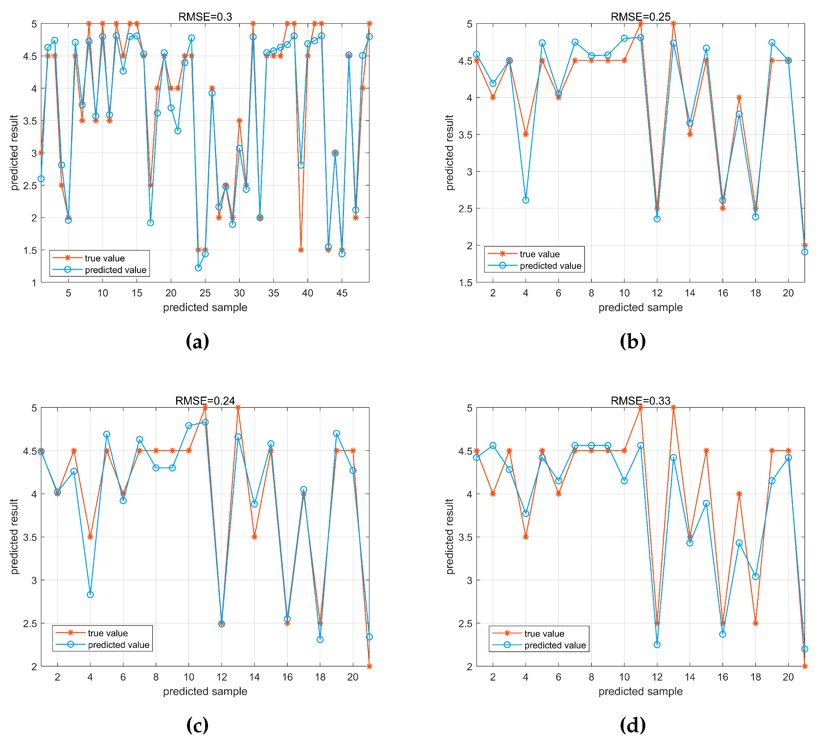
5. Conclusions
Author Contributions
Funding
Institutional Review Board Statement
Informed Consent Statement
Data Availability Statement
Conflicts of Interest
References
- Yu, X.; Wang, H. Support vector machine classification model for color fastness to ironing of vat dyes. Textile Research Journal 2021, 91, 1889–1899. [Google Scholar] [CrossRef]
- Popa, S.; Radulescu-Grad, M.E.; Perdivara, A.; Mosoarca, G. Aspects regarding colour fastness and adsorption studies of a new azo-stilbene dye for acrylic resins. Scientific Reports 2021, 11, 5889. [Google Scholar] [CrossRef] [PubMed]
- Liu, J.; Yuan, Y.; Zhang, X.; Lixia, S. Development of intelligent grade system for textiles color fastness. Cotton Textile Technology 2019, 47. [Google Scholar]
- Huang, S.; Tu, X.; Zhou, S. Application of Kappa Coefficient Consistency test in visual evaluation of color fastness. Knitting Industries 2022, p. 5.
- Development of a low-cost UV-Vis spectrophotometer and its applicatiorn for the detection of mercuric ions assisted by chemosensors. Sensors 2020, 20, 906. [CrossRef]
- Deidda, R.; Sacre, P.Y.; Clavaud, M.; Coïc, L.; Avohou, H.; Hubert, P.; Ziemons, E. Vibrational spectroscopy in analysis of pharmaceuticals: Critical review of innovative portable and handheld NIR and Raman spectrophotometers. TrAC Trends in Analytical Chemistry 2019, 114, 251–259. [Google Scholar] [CrossRef]
- An, Y.; Xue, W.; Ding, Y.; Zhang, S. Evaluation of textile color rubbing fastness based on image processing. Journal of Textile Research 2023, 43, 131–137. [Google Scholar]
- Salueña, B.H.; Gamasa, C.S.; Rubial, J.M.D.; Odriozola, C.A. CIELAB color paths during meat shelf life. Meat science 2019, 157, 107889. [Google Scholar] [CrossRef]
- Lin, C.J.; Prasetyo, Y.T.; Siswanto, N.D.; Jiang, B.C. Optimization of color design for military camouflage in CIELAB color space. Color Research & Application 2019, 44, 367–380. [Google Scholar]
- Cui, G.; Luo, M.; Rhodes, P.; Rigg, B.; Dakin, J. Grading textile fastness. Part 2; Development of a new staining fastness formula. Coloration technology 2003, 119, 219–224. [Google Scholar] [CrossRef]
- Cui, G.; Luo, M.; Rigg, B.; Butterworth, M.; Dakin, J. Grading textile fastness. Part 3: Development of a new fastness formula for assessing change in colour. Coloration technology 2004, 120, 226–230. [Google Scholar] [CrossRef]
- Zheng, C. Discussion on Evaluation of Color Fastness Grade of Fabrics by Image Method. Light and Textile Industry and Technology 2010, 39, 3. [Google Scholar]
- Zhang, Q.; Liu, J.; Gao, W. Grade evaluation of color fastness to laundering based on image analysis. Journal of Textile Research 2013, 34, 100–105. [Google Scholar]
- Liang, J.; Xin, L.; Zuo, Z.; Zhou, J.; Liu, A.; Luo, H.; Hu, X. Research on the deep learning-based exposure invariant spectral reconstruction method. Frontiers in Neuroscience 2022, 16, 1031546. [Google Scholar] [CrossRef]
- Zhao, Y.; Po, L.M.; Yan, Q.; Liu, W.; Lin, T. Hierarchical regression network for spectral reconstruction from RGB images. In Proceedings of the Proceedings of the IEEE/CVF Conference on Computer Vision and Pattern Recognition Workshops, 2020, pp. 422–423.
- Liang, J.; Wan, X. Optimized method for spectral reflectance reconstruction from camera responses. Optics Express 2017, 25, 28273–28287. [Google Scholar] [CrossRef]
- Xiao, K.; Zhu, Y.; Li, C.; Connah, D.; Yates, J.M.; Wuerger, S. Improved method for skin reflectance reconstruction from camera images. Optics Express 2016, 24, 14934–14950. [Google Scholar] [CrossRef]
- Kert, M.; Gorjanc, M. The study of colour fastness of commercial microencapsulated photoresponsive dye applied on cotton, cotton/polyester and polyester fabric using a pad-dry-cure process. Coloration Technology 2017, 133, 491–497. [Google Scholar] [CrossRef]
- Sezgin Bozok, S.; Ogulata, R.T. Effect of silica based sols on the optical properties and colour fastness of synthetic indigo dyed denim fabrics. Coloration Technology 2021, 137, 209–216. [Google Scholar] [CrossRef]
- Kumar, R.; Ramratan, K.A.; Uttam, D. To study natural herbal dyes on cotton fabric to improving the colour fastness and absorbency performance. J Textile Eng Fashion Technol 2021, 7, 51–56. [Google Scholar]
- Liang, J.; Xiao, K.; Pointer, M.R.; Wan, X.; Li, C. Spectra estimation from raw camera responses based on adaptive local-weighted linear regression. Optics express 2019, 27, 5165–5180. [Google Scholar] [CrossRef]
- Liu, Y.; Li, J.; Wang, X.; Li, X.; Song, Y.; Li, R. A study of spectral reflectance reconstruction using the weighted fitting algorithm based on the Sino Colour Book. Coloration Technology 2023. [Google Scholar] [CrossRef]
- Han, J.X.; Ma, M.Y.; Wang, K. Product modeling design based on genetic algorithm and BP neural network. Neural Computing and Applications 2021, 33, 4111–4117. [Google Scholar] [CrossRef]
- Song, S.; Xiong, X.; Wu, X.; Xue, Z. Modeling the SOFC by BP neural network algorithm. International Journal of Hydrogen Energy 2021, 46, 20065–20077. [Google Scholar] [CrossRef]
- Li, Y.; Liu, P.; Zhou, J.; Ren, Y.; Jin, J. Center extraction of structured light stripe based on back propagation neural network. Acta Optica Sinica 2019, 39, 1212005. [Google Scholar]
- Luo, Y.; Pei, L.; Zhang, H.; Zhong, Q.; Wang, J. Improvement of the rubbing fastness of cotton fiber in indigo/silicon non-aqueous dyeing systems. Polymers 2019, 11, 1854. [Google Scholar] [CrossRef] [PubMed]
- Lei, Z. Study on Test of Color Fastness to Rubbing of Textiles 2020. 793, 012017.
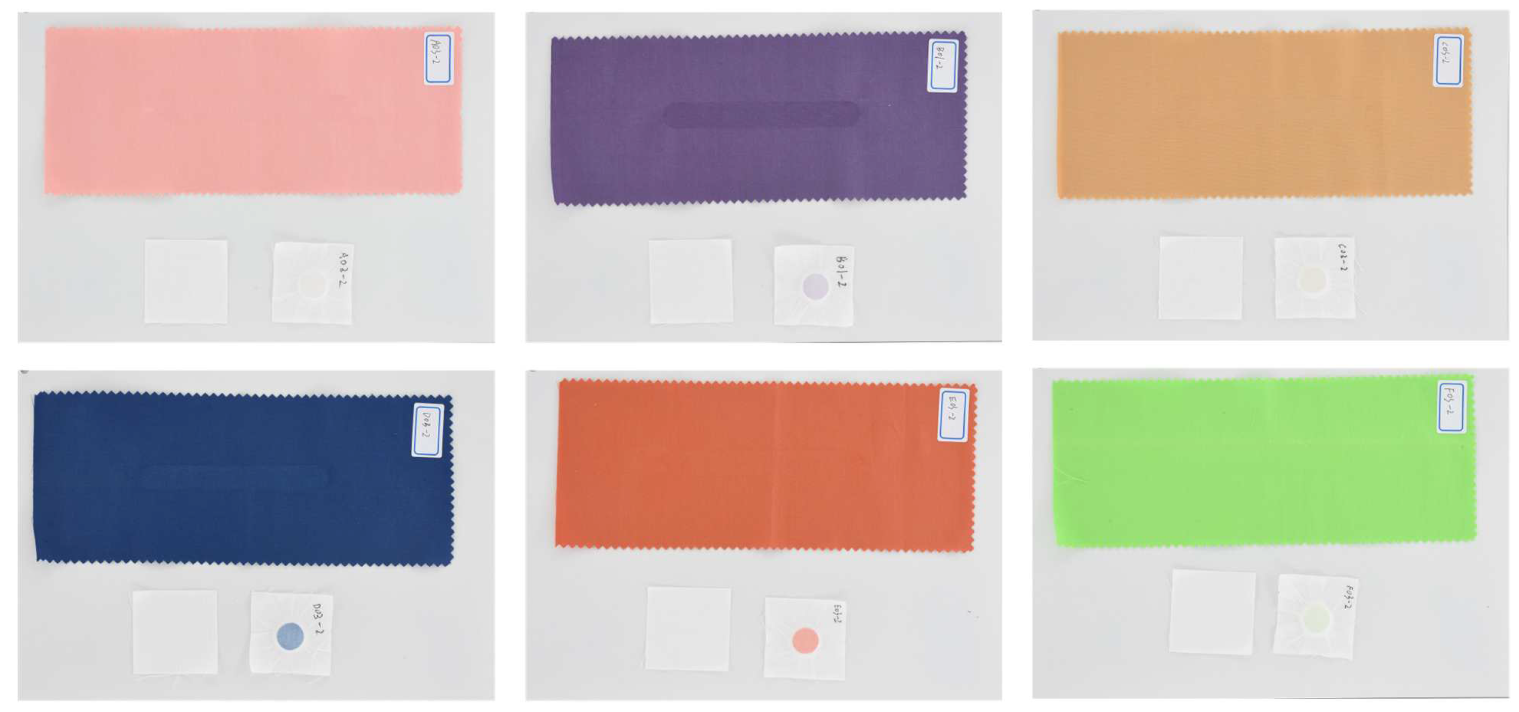
| Texture | 100% cotton twill |
| Size | 10*25cm |
| Yarn count | 40 counts |
| Density | 133*72 |
| Color | pink, purple, yellow, blue, orange, green |
| Model | Unstandardized Coefficients | Standardized Coefficient | t | Significance (p-Value) | Covariance Statistics | ||
|---|---|---|---|---|---|---|---|
| B | Standard Error | Tolerance | VIF | ||||
| Constant | -0.292 | 0.048 | -6.088 | 0.000 | |||
| L | -0.042 | 0.009 | -0.550 | -4.730 | 0.000 | 0.744 | 1.344 |
| a | -0.028 | 0.014 | -0.281 | -2.037 | 0.046 | 0.527 | 1.896 |
| b | -0.001 | 0.012 | -0.008 | -0.057 | 0.954 | 0.498 | 2.010 |
| Curve Fitting | Fitting Equation | Correlation coefficient |
|---|---|---|
| third-order polynomial | D = p1*x + p2*x + p3*x + p4 | R=0.99 |
| p1 = -1.72e-05 | ||
| p2 = 0.0029 | ||
| p3 = -0.17 | ||
| p4 = 4.97 |
| Sample No. | Visual result | BP Model | Color Difference Conversion | Curve Fitting |
|---|---|---|---|---|
| 1 | 4.5 | 4.58 | 4.49 | 4.42 |
| 2 | 4 | 4.18 | 4.02 | 4.56 |
| 3 | 4.5 | 4.49 | 4.26 | 4.28 |
| 4 | 3.5 | 2.61 | 2.83 | 3.77 |
| 5 | 4.5 | 4.73 | 4.69 | 4.42 |
| 6 | 4 | 4.04 | 3.92 | 4.15 |
| 7 | 4.5 | 4.74 | 4.63 | 4.56 |
| 8 | 4.5 | 4.56 | 4.3 | 4.56 |
| 9 | 4.5 | 4.57 | 4.3 | 4.56 |
| 10 | 4.5 | 4.79 | 4.79 | 4.15 |
| 11 | 5 | 4.81 | 4.83 | 4.56 |
| 12 | 2.5 | 2.35 | 2.49 | 2.25 |
| 13 | 5 | 4.73 | 4.66 | 4.42 |
| 14 | 3.5 | 3.65 | 3.88 | 3.43 |
| 15 | 4.5 | 4.66 | 4.58 | 3.89 |
| 16 | 2.5 | 2.60 | 2.55 | 2.37 |
| 17 | 4 | 3.77 | 4.05 | 3.43 |
| 18 | 2.5 | 2.38 | 2.31 | 3.04 |
| 19 | 4.5 | 4.74 | 4.7 | 4.15 |
| 20 | 4.5 | 4.50 | 4.27 | 4.42 |
| 21 | 2 | 1.91 | 2.34 | 2.2 |
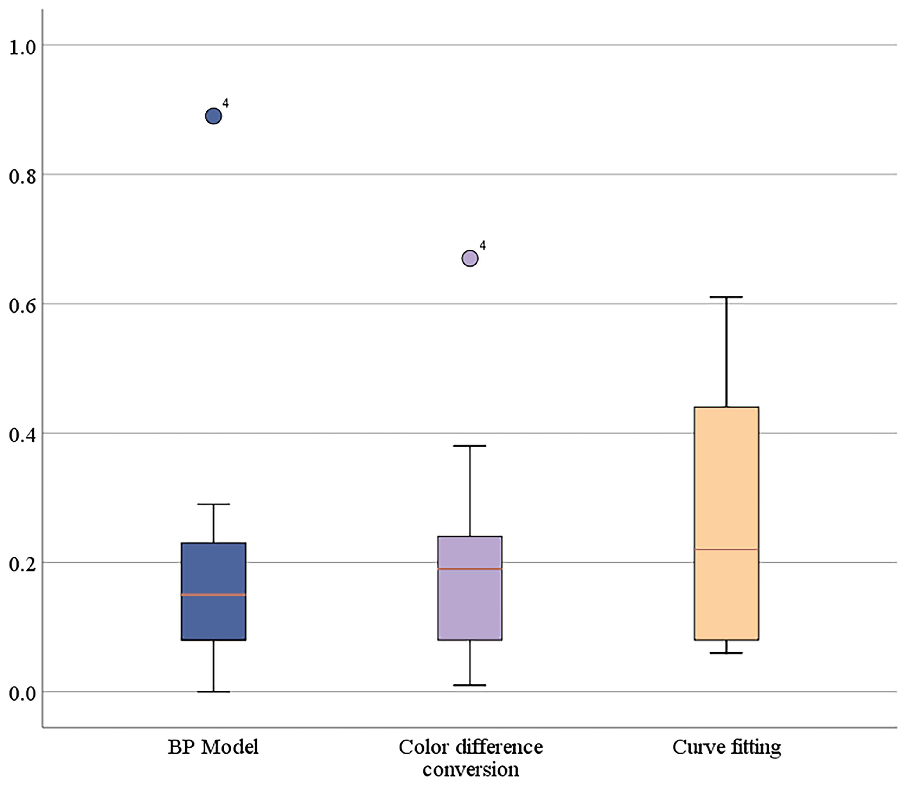
| BP Model | Color Difference Conversion | Curve Fitting | |
|---|---|---|---|
| RMSE | 0.25 | 0.24 | 0.33 |
| Maximum Error | 0.89 | 0.67 | 0.61 |
| Minimum Error | 0 | 0.01 | 0.06 |
| Median Error | 0.15 | 0.19 | 0.22 |
Disclaimer/Publisher’s Note: The statements, opinions and data contained in all publications are solely those of the individual author(s) and contributor(s) and not of MDPI and/or the editor(s). MDPI and/or the editor(s) disclaim responsibility for any injury to people or property resulting from any ideas, methods, instructions or products referred to in the content. |
© 2023 by the authors. Licensee MDPI, Basel, Switzerland. This article is an open access article distributed under the terms and conditions of the Creative Commons Attribution (CC BY) license (http://creativecommons.org/licenses/by/4.0/).


