
Submitted:
01 August 2023
Posted:
03 August 2023
You are already at the latest version
Abstract
In this paper, a robust nonlinear dynamic controller is designed for a wind turbine with a permanent magnet synchronous generator. The wind turbine is subject to variations in all the parameters appearing in its mathematical model. Furthermore, the wind velocity is considered unavailable for direct measurement. This situation is of particular interest in practical applications, where only the nominal parameter values are known, and accurate wind velocity measurement is challenging due to perturbations caused by the turbine itself, even with appropriate sensors. The problem addressed in this work involves tracking the reference angular velocity corresponding to the wind velocity. To achieve accurate tracking, appropriate compensation of the perturbation terms resulting from parameter uncertainties and wind estimation errors is required. To address this problem, an estimator of the wind velocity is utilized, along with high–order sliding mode parameter estimators, to ensure high–performance operation of the turbine.
Keywords:
Wind Turbine
; Nonlinear Control
; Parameter Variations
; High–Order Sliding Mode
1. Introduction
Recently, Wind Turbine Convertion Systems (WTCSs) have received great attention by the scientific community for the exploitation of renewable energies. Many works available in the literature focus on the nonlinear control of small and large scale wind energy generation systems. In particular, Permanent Magnet Synchronous Generators (PMSGs) are used as wind turbine generators due to their advantages regarding the efficient and reliable performance. These advantages are linked to their properties of self–excitation and of low speed, which results in direct–drive WTCSs. In fact, PMSGs have a simpler mechanical structure, may have direct coupling to the wind turbine shaft avoiding gears, and do not need an external excitation system, so avoiding the corresponding copper losses.
The aim is to maximize the power generated by the Wind Turbine (WT) under the condition of variable wind speed. This is achieved maintaining the so–called tip–speed ratio, i.e. the ratio between the blade tip linear velocity and the wind velocity, at an optimal value. For a given wind velocity, this optimal value of the tip–speed ratio corresponds to a certain angular velocity, which is considered as a reference to be tracked. Therefore, the problem of the optimal energy extraction can be expressed as a tracking problem of the reference angular velocity corresponding to the given wind velocity.
This tracking problem is here solved in the presence of some difficulties that normally arise in practical cases. The first difficulty is that the measurement of the real wind velocity value is unrealistic for industrial WTs. In fact, the wind velocity can not be measured with accuracy since, even in the presence of appropriate sensors, the wind velocity field is perturbed by the turbine itself. A second difficulty arises from the fact that the parameters appearing in the mechanical and electrical equations are usually subject to parameter variations or uncertainties. Examples are the winding resistance, air density, etc., which are subject to variations, and the PMSG rotor inertia, friction, etc., which are known with a certain uncertainty. In practice, only the nominal values of these parameters can be assumed known. In order to solve the tracking problem in the presence of these two difficulties, in this work an estimator of the wind velocity is used. Furthermore, high–order sliding mode estimators are used to estimate the perturbation terms arising in the dynamical equations due to the parameter uncertainties. This allows a compensation of the perturbation terms due to the parameter uncertainties and of the wind estimation error, ensuring an accurate tracking of the reference angular velocity.
Regarding parameter variations and uncertainties, the First Order Sliding Mode (FOSM) technique constitutes an interesting methodology that can be used to compensate their effects. This is achieved thanks to the inherent robustness of this technique [1]. Examples of FOSM control of WTs are given in [2,3,4] which presented robust controllers designed for variable speed WTs with doubly fed induction generators. A FOSM control is also designed in [5] for a turbine model considering the mechanical dynamics only, along with a modified Newton–Rapshon algorithm to estimate the wind speed. Another FOSM controller, using the blade pitch as input, was designed in [6] in the presence of uncertainties, in order to regulate the rotor speed to a fixed rated value. A FOSM control for a variable speed WT with PMSG was considered in [7], under the assumption of measurability of the wind speed. In [8], an algorithm based on the combination of FOSM and fractional–order SM was proposed, where the latter ensures finite–time convergence to zero of the angular velocity tracking error. In [9], a novel robust FOSM control was proposed, using nonlinear perturbation observers for WTs with a doubly–fed induction generator. Finally, an integral terminal FOSM controller was proposed in [10] to enhance the power quality of WTs under unbalanced voltage conditions.
FOSM control schemes may suffer from the well–known chattering problem, i.e. high frequency oscillations due to actuator bandwidth limitations, unable to reproduce exactly the sign “function” used in FOSM, which has clear negative consequences. In order to overcome this difficulty, and to consider SM surfaces with relative degree greater than one [11], High–Order Sliding–Mode (HOSM) techniques can be used. These techniques, also called Super–Twisting Sliding–Mode (STSM) techniques, have other appealing properties, since they ensure finite–time convergence to the origin, and robustness with respect to perturbation acting on the system. Such techniques were developped starting from the seminal paper of [12] and successively fully developped in succesive papers [13,14,15,16,17,18,19]. HOSM techniques were first used for smooth control systems, and successively as finite–time differentiators. They were also applied successfully to a number of applications [11,20,21,22,23,24,25,26,27]. Recently, extensive research has been undertaken to control PMSG for wind energy conversion applications using HOSM techniques. In [28], an efficient controller based on a HOSM was proposed and applied to a PMSG. [29] presented an output HOSM power control of a Wind Energy Conversion System (WECS) based on a PMSG, which integrates a stand–alone hybrid system for the optimum power conversion and power regulation operational mode. In [4,30], a HOSM control scheme was developed for a PMSG, consisting of a robust aerodynamic torque observer based on the super–twisting algorithm in order to eliminate the sensors for the wind speed measurement, and a robust wind turbine speed control to regulate the rotor currents. [31] proposed an adaptive sliding mode speed control algorithm with an integral–operation sliding surface for a variable speed wind energy experimental system. Besides, the proposed controller includes an estimator that deals with the unknown turbine torque and inaccuracies in the mathematical model of the system and attempts to achieve zero steady-state error. [32] present a Super Twisting (ST) algorithm using an Adaptive Second-Order Sliding Mode Control (SOSMC) to derive a robust and fast current control for PMSG–based WECS. The aim of the controller is to force the PMSG to deliver the requested power to the grid via controlling the winding current. A conventional sliding mode (SMC) and second-order sliding mode (SOSMC) control schemes based on pulse width modulation (PWM) for the rotor side converter (RSC) and grid side converter (GSC) feeding a doubly fed induction generator (DFIG) are presented in [33,34]. In is worth nothing that all these works do not deal with parameter uncertainties in the PMSG dynamics.
In this paper, a robust nonlinear dynamic controller is designed for a WT with a PMSG, which guarantees the maximization of the power extracted by the WT from the wind. The control objective is to track an appropriate angular velocity signal, ensuring the asymptotic stability of the closed–loop system despite variations in all the parameters present in the WT mathematical model. The original contributions of this paper are centered around solving the tracking problem in the presence of the following factors:
- Unknown wind velocity, which is estimated based on measurements of the produced power.
- Parameter variations and uncertainties in the WT model, estimated using high–order sliding mode estimators.
It is worth noting that the unavailability of wind velocity measurement is not considered in the available literature.
2. Mathematical Model of a WT
The power extracted by the WT from the wind is given by [35]
where is the air density, R is the WT rotor radius, is the wind speed, is the turbine shaft speed, and is the tip speed ratio, with the tip speed of the turbine blade. Moreover, is the power coefficient, depending on the blade design. The power coefficient is function of the blade pitch angle and of the tip speed ratio . It represents the turbine efficiency to convert the kinetic energy of the wind into mechanical energy. The power coefficient is a nonlinear function of which, for , can be approximated as [36,37]
where are experimental coefficients depending on the shape of the blade and on its aerodynamic performance.
To maximize the power generated by the WT for a given wind velocity , one has to maximize the power coefficient . Since this latter depends on and , also its maximum depends on these two variables. Nevertheless, usually is changed occasionally, and in the following it will be considered constant and equal to a value deg. Therefore, the maximization of is achieved maximizing , which has its maximum for . Obviously, the same reasoning can be followed for other values of the blade pith angle .
The model of a PMSG in the reference frame, rotating synchronously with the generator rotor, is [37]
where , are the d, q–axis stator currents, , are the d, q–axis stator voltages, is the winding resistance and is the winding inductance on axis d and q, is the flux linkage of the permanent magnet, is the electrical angular speed of the generator rotor, and p is the number of pole pairs. In the mechanical equation, is the electrical torque, with the torque constant. The developed torque of the motor is proportional to the current because of the assumption that there is no reluctance torque in the considered PMSG. Furthermore, J is the mechanical inertia, and f is the coefficient of the viscous friction. The torque extracted from the wind is . It summarizes the effect of the aerodynamic torque, generally known with large inaccuracy.
In this work, all the parameters appearing in the electric and mechanical dynamics (1) are assumed to be subject to variation. Let , , , , , be the nominal values of , L, , , J, f, and
the nominal value of , where is the nominal value of , is the nominal value for R, , and is the nominal function
with , the nominal values of . Finally, the nominal value of is .
In what follows it will be assumed that the parameter variations , , , , , , are bounded by certain values , , , , , , , respectively. This is an acceptable assumption from a physical point of view.
The control problem consists of designing a dynamic controller to track a reference angular velocity , which will be determined later, in the presence of uncertainties on all the parameters appearing in the model.
Considering the maximization of , which is obtained imposing the value , and using the definition of the tip speed ratio, one obtains the reference angular velocity , that should be imposed. However, one observes that such a function is not known, as and are not known. Therefore, in the following an estimation of the wind velocity will be determined, while will be substituted by its (known) nominal value .
3. Design of the Dynamic Controller for the Tracking of the Angular Velocity Reference
The first step in the design of the desired controller is to estimate the wind velocity, in order to obtain a known angular velocity reference.
3.1. Design of the Wind Velocity Estimator
As already commented, the measurement of the real velocity value is unrealistic for industrial WTs. In the following, the wind velocity can be estimated from the measurement of the produced power . In fact, considering the nominal value and the function
it is possible to determine the value of imposing . To this aim, among the other methods, a Newton–Raphson method can be used [38]. Hence, one can look for the solutions of the equation considering the iterative estimations
for a fixed integer , where
From the definition of , and using the estimation , one computes the wind velocity estimation
and the following reference angular velocity
can be defined, with the (known) maximum value of . This is the reference angular velocity that the controller has to track, in the presence of parameter uncertainties.
3.2. Design of the Dynamic Controller for the Tracking of the Angular Velocity Reference
Given the model (1), and considering the nominal values , , , , , , one obtains the following model
with the perturbation terms
The final perturbation term for the dynamics of will be given by the sum of and additional terms arising from the derivative of the reference imposed on . This will become clearer in the subsequent computations.
The following result solves the posed control problem for the system (4).
Theorem 1.
If the signals , , ω are measurable, the dynamic controller
, with , , , and
bounded function with bounded derivative, and with
ensures that the tracking error , converges to zero asymptotically. Moreover, the errors , converge asymptotically to zero. ⋄
Proof.
Let us define the angular velocity tracking error . The dynamics of are
where , with as in (7), and . The dynamics of are
with the derivative of given by
, as in (8), and with the (unknown) perturbation term given by
Using the controller (5), one works out
with . Considering (9), (10), one finally gets the coupled dynamics
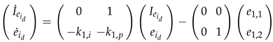
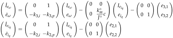 where the dynamics of the errors , , , , are
The errors , tend to zero in finite time. The proof of the global convergence to the origin in finite time of , can be demonstrated with Lyapunov arguments [39,40], considering the Lyapunov candidate
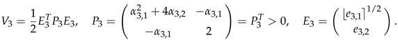
This candidate is continuous but not differentiable. As explained in [39], the use of the classical version of Lyapunov’s theory [41], instead of nonsmooth versions [42,43], is allowed since is differentiable almost everywhere, i.e., except when . The fact that the trajectories of (12) may pass through for time instants constituting a set of null measure before reaching the origin from a certain finite-time instant on allows using the classical version of Lyapunov’s theory. Therefore, considering the necessary modifications with respect to the proof given in [39]
where
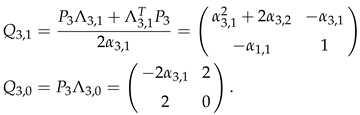
We will proof later that, with the proposed controller, remains bounded, with for all time instants. To take into account the perturbation , can be bounded as follows
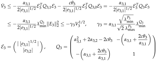 with α3,1>0, Q3>0 under the conditions (6), and
  Also here, slight modifications with respect to the proof of [39] were necessary. This proves the finite−time convergence of E3 to the origin.
Also here, slight modifications with respect to the proof of [39] were necessary. This proves the finite−time convergence of E3 to the origin.With the same arguments, also the errors , can be proved to tend to zero in finite time, considering the Lyapunov candidate

Also in this case it will be shown that remains bounded, with .
Since , , , tend to zero in finite time, the tracking error dynamics (11) has the origin globally asymptotically stable, namely , , , tend to zero asymptotically.
Finally, considering the expression of the reference as in (7) and the control as in (5), for the error one obtains
where
With the same arguments used before, , tend to zero in finite time, since . As a consequence, the closed–loop dynamics
 has the origin globally asymptotically stable, namely tend to zero asymptotically.
We can now show what stated before, namely, that remain bounded for all time instants. In fact, since the initial tracking errors , , are finite, so are
and
and the right sides of the equations (4) for . Since the functions involved are also locally Lipschitz, this remains true for finite time intervals , . This implies that the dynamics (12), (15) converge to zero for . This reasoning can be iterated, so that the local Lipschitzianity implies that remain bounded for all time instants.
This concludes the proof. □
4. Simulation results
The proposed dynamic controller (5) has been tested by simulation using the mathematical model (1). The simulation of the wind speed profile was considered from realistic measurements [44], shown in Figure 1. The main parameters of the considered WT are shown in Table 1. Variations of some of these mechanical and electrical parameters have been considered, as indicated in Table 2.
Some of the performances achieved by the proposed controller (5) using the gains given in Table 3 have been reported in Figure 2, Figure 3 and Figure 4 with the initial conditions A, A, rad/s. Figure 2 show the stator voltages and , while Figure 3 shows the behavior of the d–axis stator current and its reference , the q–axis stator current and its reference , and the tracking error . Finally, Figure 4 shows the angular velocity and its reference , along with the tracking error . The parameter estimations, shown in Figure 5 and Figure 6, have been determined considering the gains reported in Table 4. The reported simulation results demonstrate the accurate tracking achieved by the proposed controller. These performances ensure the maximization of the power extracted by the WT from the wind.
5. Conclusions
In this work, a robust nonlinear dynamic controller has been designed for a WT with a PMSG. This controller ensures the maximization of the power extracted by the WT from the wind. To design the controller, a tracking problem was solved, ensuring the accurate tracking of an angular velocity reference for the WT blades. The wind velocity was assumed to be unavailable for direct measurement, and an estimator of the wind velocity was employed. Furthermore, a High–Order Sliding Mode (HOSM) parameter estimator was utilized to compensate for the unknown perturbation terms, resulting in high–performance control of the WT. The simulations demonstrate the good performance of the controller.
References
- V.I. Utkin, Sliding Modes in Control and Optimization, Springer–Verlag, Berlin, 1992. [CrossRef]
- Barambones O., Sliding Mode Control Strategy for Wind Turbine Power Maximization, Energies, Vol. 5, No. 7, pp.2310-2330, 2012. [CrossRef]
- Barambones and J. M. González de Durana,Wind Turbine Control Scheme Based on Adaptive Sliding Mode Controller and Observer, 2015 IEEE 20th Conference on Emerging Technologies Factory Automation (ETFA), pp. 1–7, 2015.
- Barambones and J. M. González de Durana, Second Order Sliding Mode Controller and Observer for a Wind Turbine System, 2017 IEEE International Conference on Environment and Electrical Engineering and 2017 IEEE Industrial and Commercial Power Systems Europe (EEEIC / I CPS Europe), pp. 1–6, 2017.
- Rajendran S., and Jena D., Backstepping Sliding Mode Control of a Variable Speed Wind Turbine for Power Optimization, Journal of Modern Power Systems and Clean Energy, Vol. 3, No. 3, pp. 402–410, 2015. [CrossRef]
- M.L., Ippoliti G., and Orlando G., A Sliding Mode Pitch Controller forWind Turbines Operating in High Wind Speeds Region, in Proceedings of International Conference on Control, Decision and Information Technologies, pp. 1–6, 2017. [CrossRef]
- Gajewski P., and Pie ´nkowski K., Analysis of Sliding Mode Control of Variable Speed Wind Turbine System with PMSG, in International Symposium on Electrical Machines (SME), pp. 1–6, 2017. [CrossRef]
- Ardjal A., Mansouri R. and Bettayeb M., Fractional sliding mode control of wind turbine for maximum power point tracking, Transactions of the Institute of Measurement and Control, Vol. 41, No. 2, pp. 447-457, 2018. [CrossRef]
- Yang B., Yu T., Shu H., Dong J., and Jiang L., Robust sliding–mode control of wind energy conversion systems for optimal power extraction via nonlinear perturbation observers, Applied Energy, Vol. 210, pp. 711-723, 2018. [CrossRef]
- Mohammad J. M., Afef F., A Sliding Mode Approach to Enhance the Power Quality of Wind Turbines Under Unbalanced Voltage Conditions, IEEE/CAA Journal of Automatica Sinica, Vol. 2, No. 2, 2019. [CrossRef]
- Fridman L, Moreno J, Iriarte R. Sliding Modes after the first Decade of the 21st Century: State of the Art. Lecture Notes in Control and Information Sciences 412. Springer–Verlag Berlin 2011.
- Emelyanov SV, Korovin SK, Levantovsky LV. Higher Order Sliding Regimes in the Binary Control Systems. Soviet Physics 1986; 31(4): pp. 291–3.
- Edwards C, Spurgeon SK. Sliding Mode Control: Theory and Application 1999; Taylor and Francis Ltd., London.
- Bartolini G, Pisano A, Usai E. First and Second Derivative Estimation by Sliding Mode Technique. Journal of Signal Processing 2000; 4: pp. 167–76.
- Fridman L, Levant A. Higher Order Sliding Modes. Sliding Mode Control in Engineering 2002: Marcel Dekker, New York, pp. 53–101, 2002.
- Floquet T, Barbot JP, Super Twisting Algorithm based Step–by–Step Sliding Mode Observers for Nonlinear Systems with Unknown Inputs. In: Special Issue of International Journal of Systems Science on Advances in Sliding Mode Observation and Estimation 2007; 10(10): pp. 803–15.
- Levant A. Higher–Order Sliding Modes, Differentiation and Output Feedback Control. International Journal of Control 2003; 76(9,10); pp. 924–941.
- Fridman L, Shtessel Y, Edwards C, Yan XG. Higher–Order Sliding–Mode Observer for State Estimation and Input Reconstruction in Nonlinear Systems. International Journal of Robust and Nonlinear Control 2008; 18(4,5): pp. 399–413. [CrossRef]
- Levant A. Homogeneity Approach to High–Order Sliding Mode Design. Automatica 2005; 41(5): pp. 823–30. [CrossRef]
- Basin MV, Yu P, Shtessel YB. Hypersonic Missile Adaptive Sliding Mode Control Using Finite– and Fixed–Time Observers. IEEE Transactions on Industrial Electronics 2018; 65(1): pp. 930–41. [CrossRef]
- Deng H, Li Q, Chen W, Zhang G. High–Order Sliding Mode Observer Based OER Control for PEM Fuel Cell Air–Feed System. IEEE Transactions on Energy Conversion 2018; 33(1): pp. 232–44. [CrossRef]
- Kommuri SK; Lee SB, Veluvolu KC. Robust Sensors–Fault–Tolerance With Sliding Mode Estimation and Control for PMSM Drives. IEEE/ASME Transactions on Mechatronics 2018; 23(1): pp. 17–28. [CrossRef]
- Pan Y, Yang C, Pan L, Yu H. Integral Sliding Mode Control: Performance, Modification, and Improvement. IEEE Transactions on Industrial Informatics 2018; 14(7): pp. 3087–96.
- Panathula CB, Rosales A, Shtessel YB, Fridman LM. Closing Gaps for Aircraft Attitude Higher Order Sliding Mode Control Certification via Practical Stability Margins Identification. IEEE Transactions on Control Systems Technology 2018; 26(6): pp. 2020–34. [CrossRef]
- Liu J, Gao Y, Su X,Wack M,Wu L. Disturbance Observer Based Control for Air Management of PEM Fuel Cell Systems via Sliding Mode Technique. IEEE Transactions on Control Systems Technology 2018; pp. 1–10. [CrossRef]
- Gao Y., Liu J, Sun G, Liu M, Wu L. Fault Deviation Estimation and Integral Sliding Mode Control Design for Lipschitz Nonlinear Systems. Systems & Control Letters 2019; 123(2019): pp. 8–15.
- Van M. An Enhanced Tracking Control of Marine Surface Vessels Based on Adaptive Integral Sliding Mode Control and Disturbance Observer. ISA Transactions 2019; In Press. [CrossRef]
- Karim B., Sami B.S., and Adnane C., Higher Order Sliding mode control For PMSG in Wind power Conversion System, in Proceedings of International Conference on Control Engineering and Information Technology, pp. 1–6, 2016. [CrossRef]
- Valenciaga F., and Puleston P. F., High-Order Sliding Control for aWind Energy Conversion System Based on a Permanent Magnet Synchronous Generator, IEEE Transactions on Energy Conversion, Vol.23, No. 3, pp. 860-867, 2008. [CrossRef]
- Barambones O., and Gonzalez de Durana J. M., Adaptive sliding mode control strategy for a wind turbine systems using a HOSM wind torque observer, in IEEE International Energy Conference (ENERGYCON), pp. 1–6, 2016. [CrossRef]
- Merabet A., Adaptive Sliding Mode Speed Control for Wind Energy Experimental System, Energies, Vol. 11, No. 2238, 2018. [CrossRef]
- Matraji I., Al-Durra A., Errouissi R., Design and experimental validation of enhanced adaptive second-order SMC for PMSG-based wind energy conversion system, Electrical Power and Energy Systems, Vol. 103, No. 2018, pp. 21–30, 2018. [CrossRef]
- Fdaili M., Essadki A., Kharchouf I., and Nasser T., An overall modeling of wind turbine systems based on DFIG using conventional sliding mode and second-order sliding mode controllers, in International Conference on Wireless Technologies, Embedded and Intelligent Systems (WITS), pp.1–6. [CrossRef]
- Zargham F., Mazinan A. H., Super-twisting sliding mode control approach with its application to wind turbine systems, Energy Syst, Vol. 10, No. 1, pp. 211–229. [CrossRef]
- F.D. Bianchi, H.N.D. Battista, and R.J. Mantz, Wind Turbine Control Systems: Principles, Modelling and Gain Scheduling Design, Springer–Verlag, Berlin, Germany, 2007.
- H. Siegfried, Grid Integration ofWind Energy Conversion Systems, Wiley, New York, NY, USA, 1998.
- J. Zaragoza, J. Pou, A. Arias, C. Spiteri, E. Robles, and S. Ceballos, Study and Experimental Verification of Control Tuning Strategies in a Variable Speed Wind Energy Conversion System, Renewable Energy, Vol. 36, No. 5, pp. 1421–1430, 2011. [CrossRef]
- S. Bhowmik, R. Spee, and J.H.R. Enslin, Performance Optimization for Doubly Fed Wind Power Generation Systems, IEEE Transactions on Industrial Applications, Vol. 35, No. 4, pp. 949–958, 1999. [CrossRef]
- J. A. Moreno and M. Osorio, A Lyapunov Approach to Second–Order Sliding Mode Controllers and Observers, Proceedings of the 47th IEEE Conference on Decision and Control, Cancun, Mexico, pp. 2856–2861, 2008. [CrossRef]
- J.A. Moreno, Lyapunov Approach for Analysis and Design of Second Order Sliding Mode Algorithms, in Sliding Modes after the First Decade of the 21st Century: State of the Art, Lecture Notes in Control and Information Sciences, No. 412, M. Thoma, F. Allgöwer, M. Morari Eds., Springer–Verlag, Berlin, Germany, 2011. [CrossRef]
- H.K. Khalil, Nonlinear Systems, 3rd Edition, Prentice–Hall, Englewood Cliffs, New Jersey 2002.
- F.H. Clarke, Y. Ledyaev, R.J. Stern, and P.R. Wolenski, Nonsmooth Analysis and Control Theory, New York, Springer–Verlag, 1998. [CrossRef]
- J. Cortés, Discontinuous Dynamical Systems: A Tutorial on Solutions, Nonsmooth Analysis, and Stability, IEEE Control Systems Magazine, Vol. 28, No. 3, pp. 36–73, 2008. [CrossRef]
- Introduction to Wind speed monitoring for wind turbines (2021), Avaible in https://www.windlogger.com/blogs/news/5116392-introduction-to-wind-speed-monitoring-for-wind-turbines.
Figure 1.
Wind velocity profile .
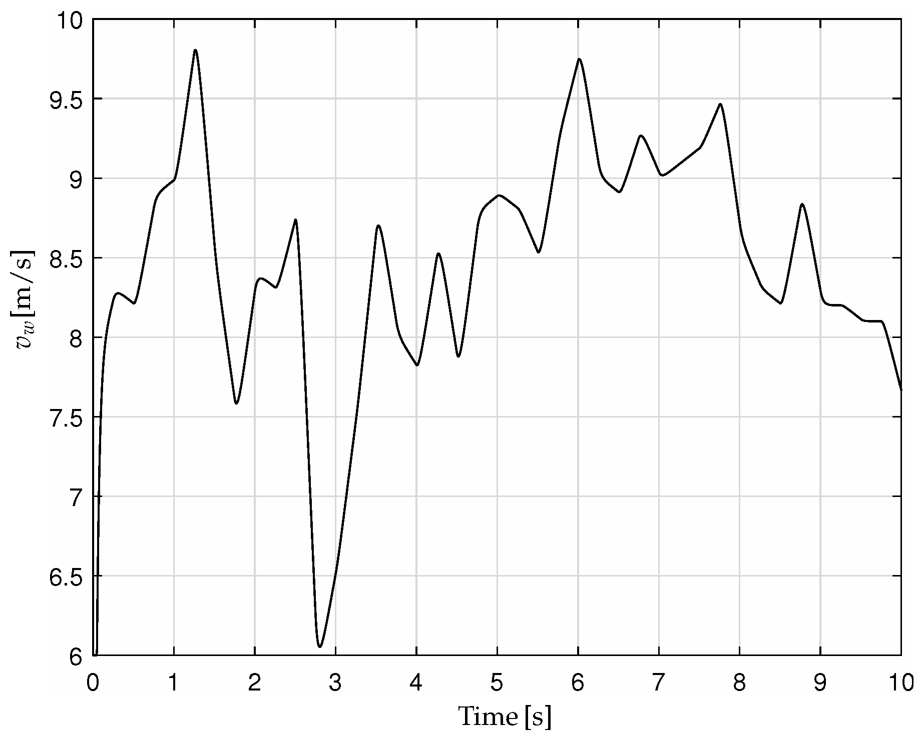
Figure 2.
a) Stator voltage ; b) Stator voltage .
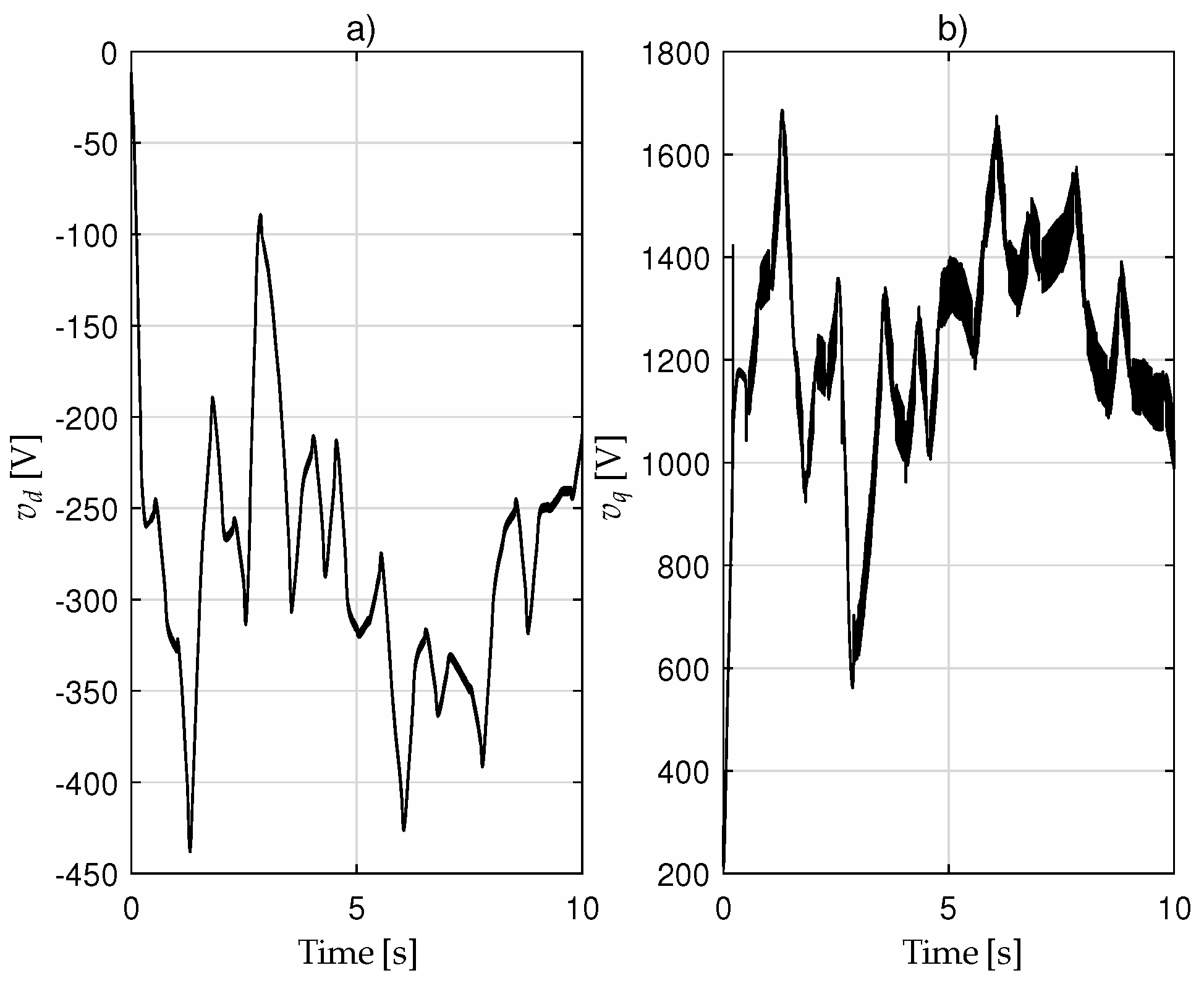
Figure 3.
a) Stator current and its reference ; b) Stator current (black) and reference (red); c) Tracking error .
Figure 3.
a) Stator current and its reference ; b) Stator current (black) and reference (red); c) Tracking error .
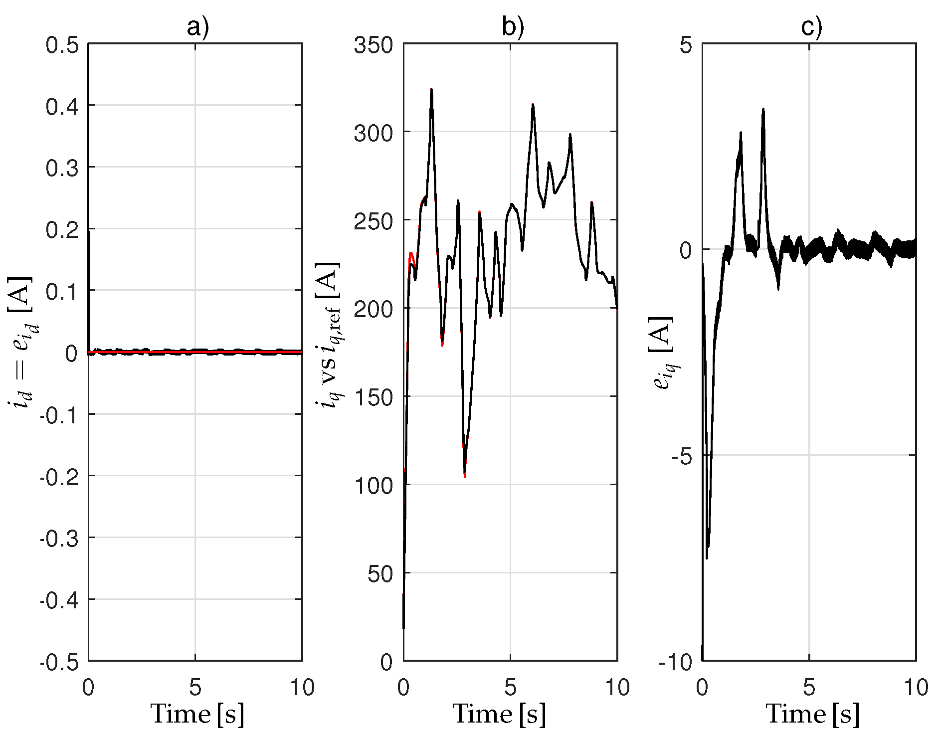
Figure 4.
a) Angular velocity (black) and reference (red); b) Tracking error .
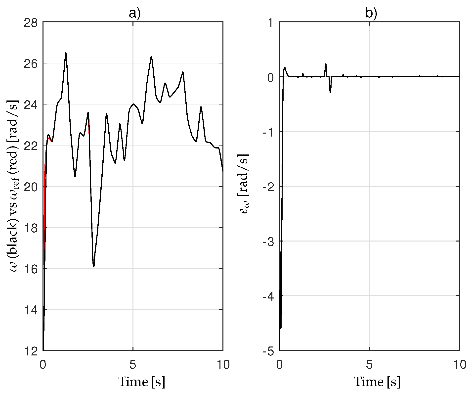
Figure 5.
Error estimations. a) (red) and tracking error (black); b) (red) and tracking error (black); c) (red) and tracking error (black); d) ; e) ; f) .
Figure 5.
Error estimations. a) (red) and tracking error (black); b) (red) and tracking error (black); c) (red) and tracking error (black); d) ; e) ; f) .
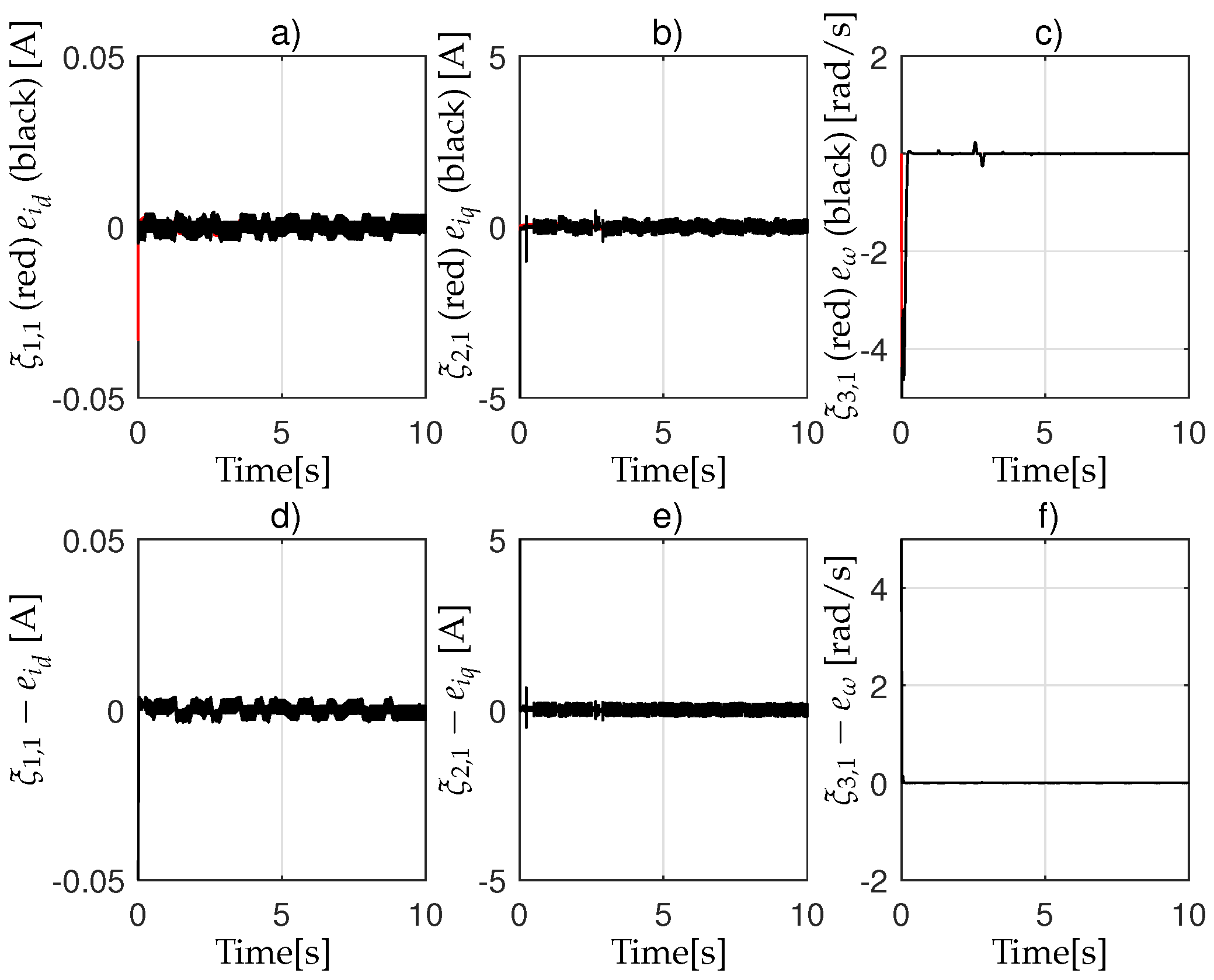
Figure 6.
Velocity error estimations. a) (red) and (black); b) (red) and (black); c) (red) and (black); d) ; e) ; f) .
Figure 6.
Velocity error estimations. a) (red) and (black); b) (red) and (black); c) (red) and (black); d) ; e) ; f) .
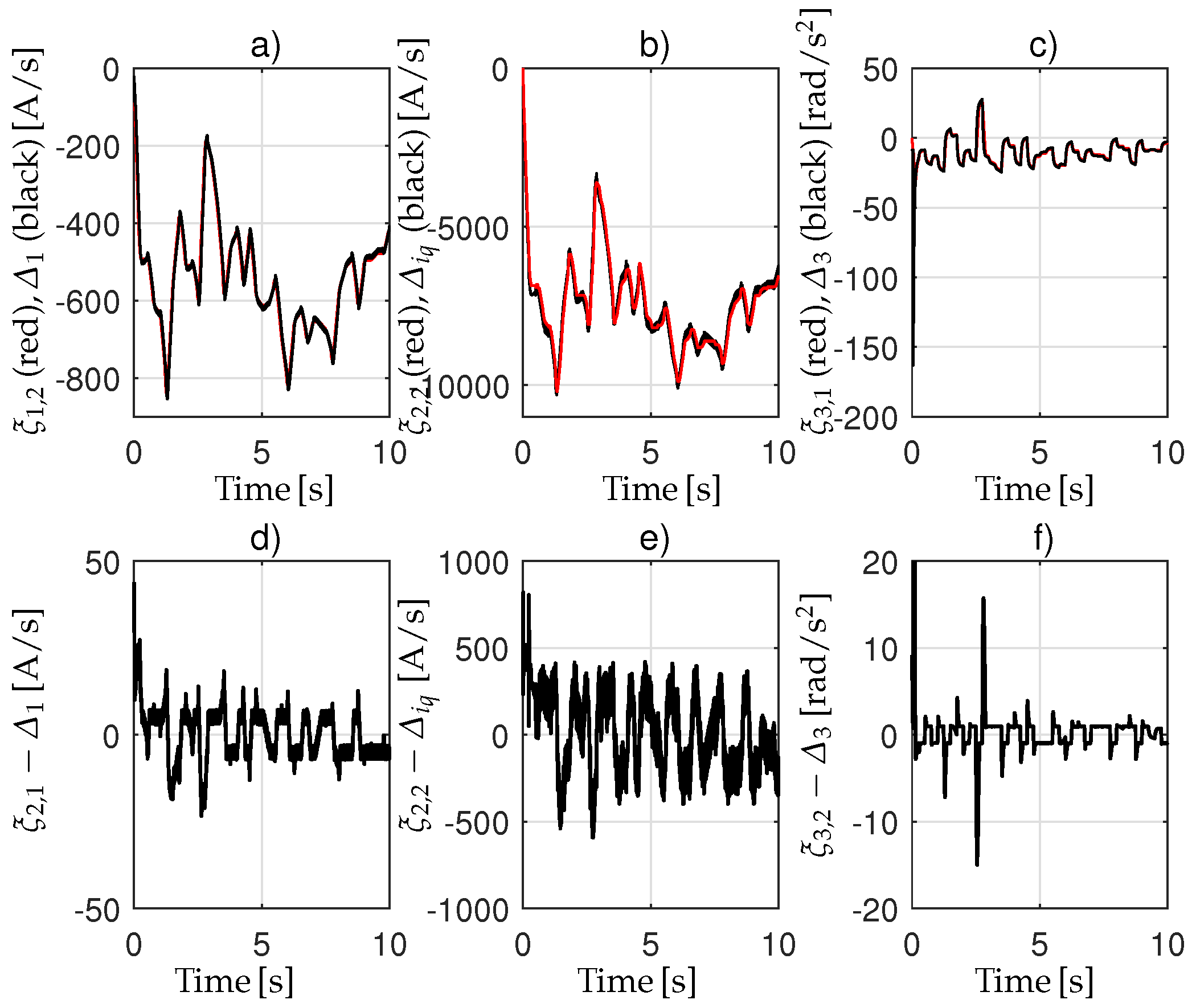

Table 1.
WT nominal values.
| Rotor radius | 46.6 m | |
| Winding resistance | 0.821 | |
| Windings inductance | 1.5731 H | |
| Flux linkage | 5.8264 Wb | |
| p | Poles number | 26 |
| Mechanical inertia | 34.6 Kg m | |
| Coefficient of viscous friction | 1.5 Kg m/s | |
| Normal air density | 1.225 |
Table 2.
WT real values.
| Kg m | Kg m/s |
Table 3.
Controller gains.
Table 4.
HOSM estimator gains.
Disclaimer/Publisher’s Note: The statements, opinions and data contained in all publications are solely those of the individual author(s) and contributor(s) and not of MDPI and/or the editor(s). MDPI and/or the editor(s) disclaim responsibility for any injury to people or property resulting from any ideas, methods, instructions or products referred to in the content. |
© 2023 by the authors. Licensee MDPI, Basel, Switzerland. This article is an open access article distributed under the terms and conditions of the Creative Commons Attribution (CC BY) license (http://creativecommons.org/licenses/by/4.0/).
Copyright: This open access article is published under a Creative Commons CC BY 4.0 license, which permit the free download, distribution, and reuse, provided that the author and preprint are cited in any reuse.


