An Improved Fault Diagnosis Approach for Pumps Based on Neural Networks with Improved Adaptive Activation Function

Due to the complex underground environment, pumping machines are prone to produce numerous failures. The indicator diagrams of faults are similar in a certain degree, which produces indistinguishable samples. As the samples increases, manual diagnosis becomes difficult, which decreases the accuracy of fault diagnosis. For accurately and quickly judging the fault type, we propose an improved adaptive activation function and apply it to five types of neural networks. The adaptive activation function improves the negative semi-axis slope of the ReLU activation function by combining the gated channel conversion unit to improve the performance of the deep learning model. The proposed adaptive activation function is compared with the traditional activation function through the fault diagnosis data set and the public data set. The results show that the activation function has better nonlinearity, can improve the generalization performance of deep learning model, the accuracy of fault diagnosis. In addition, the proposed adaptive activation function can also be well embedded in other neural networks.

Keywords:

Subject: Computer Science and Mathematics - Artificial Intelligence and Machine Learning

1. Introduction

The fault diagnosis of the pumping unit in the process of petroleum collection has been a critical research topic. Due to the complex underground environment, during the reciprocate movement of the sucker rod, there are many unknown factors, which are prone to result in the failure of the pumping machine and then form a safety hazard. Load (P) and displacement (S) are the parameters generated when the donkey head of the pumping unit moves up and down, and the closed curve formed by them is the indicator diagram. It can reflect the influence of gas, oil, water, sand, wax and other factors on pumping unit in real time [1]. If the pump is in the fault state for a long time, the wear of the pump will be aggravated and the service life of the equipment will be further reduced.

The traditional method for fault diagnosis of pumping unit is to measure the load change with displacement at the suspension point, draw the suspension point indicator diagram, and then diagnose the working condition of the pumping unit according to the shape of the indicator diagram. The disadvantages of the traditional method are as follows: first, the fault of the pumping unit is judged mainly by the method of manual identification of indicator diagram, which has great influence on human factors and low recognition accuracy. Secondly, due to the large number and wide distribution of pumped Wells, manual detection of Wells is time-consuming and laborious. However, as the complexity and high cost of pump units, there is less tolerance for performance degradation, productivity decrease, and safety hazards, therefore, it is necessary to detect and identify all potential faults rapidly [2,3]. It means that it is imperative to replace the manual fault diagnosis of the pumping unit with a computer.

With the continuous progress of deep learning technology, using deep learning technology for fault diagnosis has become a new trend. For example, Convolutional Neural Network [4] , Generation Adversarial Network [5], and Long Short Term Memory[6] et.al show superior performance in fault diagnosis.

At present, the deep learning technology used in fault diagnosis of pumping unit is to classify the indicator diagram of different kinds of faults. Automatic feature extracted from raw data is an outstanding advantage of deep learning technology, and it will not depend on the diagnostic knowledge of specialists [7].

In 2018, Y.Duan[8] proposed an improved Alexnet model to realize the automatic recognition of indicator graphs, and compared it with the current common neural network model. In 2019, J. Sang [9] proposed a PSO-BP neural network algorithm, aiming at the problems of slow convergence and unstable results of the traditional BP neural network algorithm, designed the adjustment rules of the inertia weight and learning factor of the PSO algorithm, and adjusted the weight coefficient of the output layer and the hidden layer of the BP neural network algorithm. In 2020, L.Zhang [10] used Freeman chain code and differential code to extract the characteristics of dynamometer card data of pumping unit group. Then a diagnosis model based on BP neural network was proposed, and the fault type of pump group can be automatically identified according to dynamometer card. In 2022, H.Hu[11] proposed a model based on the ResNet-34 residual network to identify the indicator diagrams, which added a residual block structure to the traditional convolutional neural network to establish a direct connection between the upper layer input and the lower layer output and achieved the recognition and classification of six power diagrams through parameter adjustment. In the same year, T.Bai[12] proposed a fault diagnosis method based on time series transformation generative adversation network (TSC-DCGAN).

Because of the complexity of pumps working conditions, there are different shapes of indicator diagrams in different working states. The indicator diagrams of different kinds of faults are similar in a certain degree thus indistinguishable samples are produced. This will lead to poor generalization ability of deep learning models and difficulty in between indistinguishable samples. The function of activation function is to carry out nonlinear transformation of data and solve the problem of insufficient expression and classification ability of linear model. If the network is all linear transformation, then the multi-layer network can be directly converted into a layer of neural network through matrix transformation. Therefore, the existence of activation function can make the deep learning model perform better with the increase of the number of layers. Therefore, we will propose a new activation function to imporove the generalization performance of the deep learning model, so that the faults of the pumping unit can be distinguished in a high dimensional space.

Rectifying linear unit(ReLU)[13], which has low computational complexity and fast convergence speed, can solve the problems of gradient disappearance and gradient saturation. In recent years, there have been many improved versions of ReLU (rectified linear unit). To solve the Dead ReLU phenomenon, the negative part of ReLU is substituted for a non-zero slope and Leaky ReLU [14] is proposed. Hence Leaky ReLU is more inclined to activate in the negative area.

In deep learning, the selection of activation function is generally determined according to the specific situation, and there is no fixed choice. As the adaptive activation function can be automatically adjusted to adapt to the network structure and practical problems, it has been widely developed. Parametric Rectified Linear Unit (PReLU) [15]is also used to solve the Dead ReLU phenomenon. The slope of the negative part can be obtained by learning from the data, rather than from defined fixed values. Therefore, PReLU has all the advantages of ReLU in theory and is more flexible than Leaky ReLU. In 2017, the Swish activation function was proposed. It has the characteristics of lower bound, no upper bound and non-monotonic. It is very smooth with its first derivative [16], and its performance is better than ReLU in many aspects. In 2021, H.Hu [17] proposed a new scheme to explore the optimal activation function with greater flexibility and adaptability by adding only a few parameters on the basis of traditional activation functions such as Sigmoid, Tanh and ReLU. This method avoids local minima by introducing a few parameters into a fixed activation function. In the same year, M.Zhao [18] used the specially designed subnetwork of Resnet-APReLU as an embedded module in order to adaptively generate the multiplicative coefficient in nonlinear transformation.

Based on the above discussions, an adaptive activation function combined with the gate-controlled channel transfer unit module (GCT)[19] is designed in this paper. The main contributions are as follows:

We propose an improved adaptive activation function. Each layer of deep learning generates different activation functions, improves the generalization performance of deep learning models, and has strong adaptability to different deep learning models.
We apply the proposed activation function to the fault diagnosis of pumping unit, so as to better extract features from the contours of the indicator diagram. The proposed activation function improves the accuracy of fault diagnosis and has a better search ability, which is verified and comprared with AlexNet[20], VGG-16[21], GoogleNet[22], ResNet[23] and DenseNet[24].
The propose activation function is extended to the public datasets CIFAR10 which proves that the proposed activation function is suitable and universal.

The rest of this paper is organized as follows. In section 2, we introduce the pumping unit data set. In section 3, we introduce the common adaptive activation function, and propose the composition of our adaptive activation function. In section 4, the experimental analysis and the discussion on the pumping unit failure data set and the public dataset are presented. In section 5, we conclude the paper.

2. Experiment Design and Measurement

2.1. Introduction to pumping unit

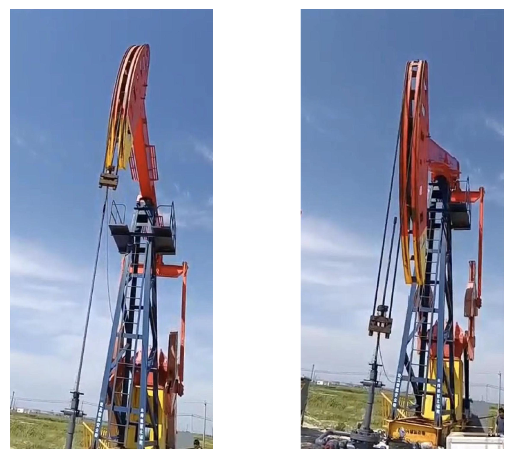
At present, about 80 % of oil wells in most oil fields in China use rod pumping equipments, and the most widely used is the beam pumping unit[25]. The failure data set of pumping unit comes from the real data generated by the pumping unit operation in a certain oil field of Northeast China. The pumping unit is a part of a rod pumping unit. Rod pumping equipment is mainly composed of three parts: oil pumping unit, well pumping pump and sucker rod. The Rod pumping equipment is shown in Figure 1.

The pumping unit is driven by a motor and through the reducer transmission system and the execution system, the rod and the pump plunger are driven to move up and down, and finally the crude oil is lifted from the well to the surface. The operation of the pumping unit is shown in Figure 2.

2.2. Fault types of pumping unit

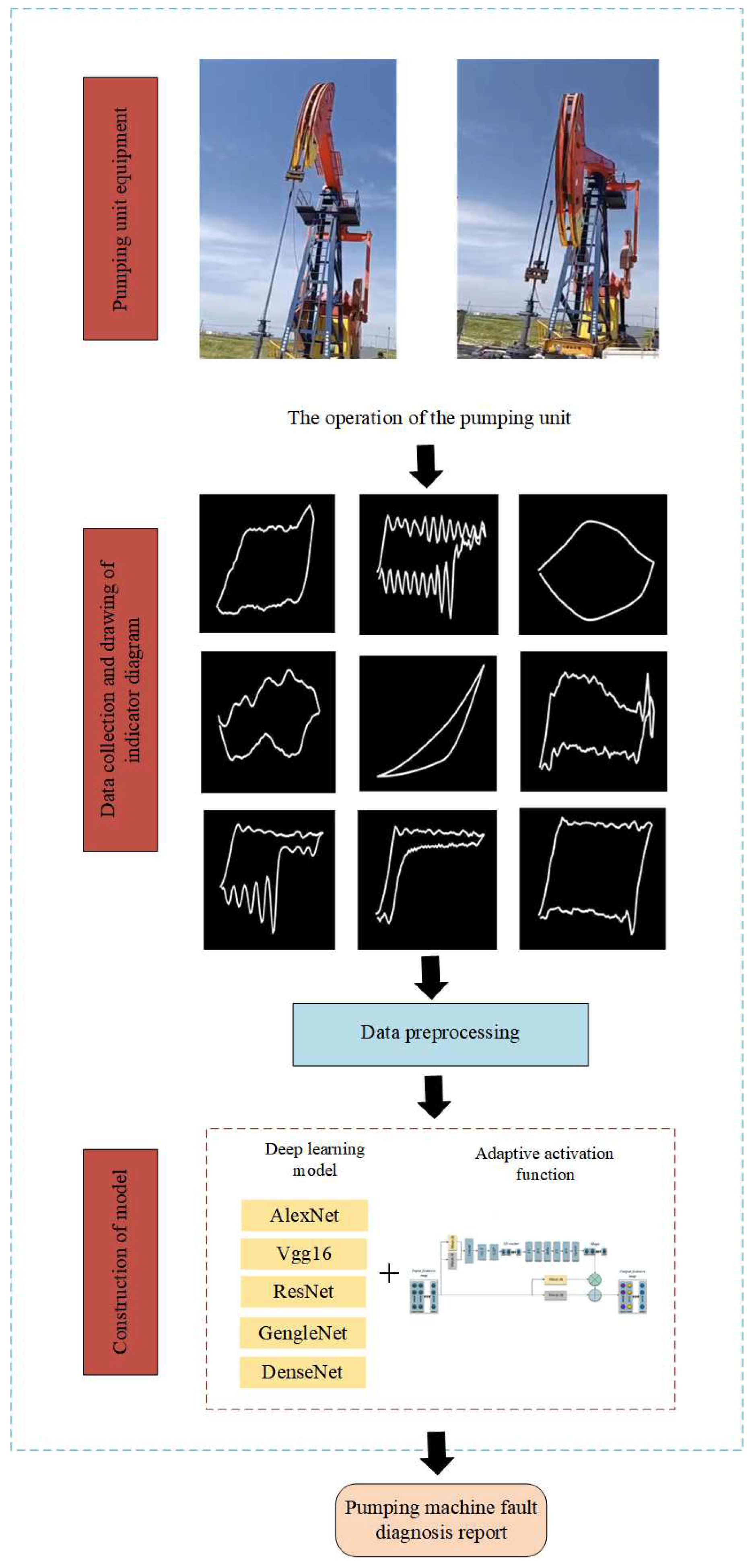
The fault data set of pumping unit consists of nine types of indicator diagrams: normal, insufficient fluid supply, contain sand, piston stuck, gas influence, pump up touch, pump down touch, double valve leakage, and pumping rod detachment. The following details will be introduced:

Normal

The pump work diagram made by normal operation refers to the position shift of the end suspension point relative to the lower dead point as the transverse setting mark, the self-weight force of the rod and the cumulative load received by the pump plug as the longitudinal setting mark. Drawn in parallel quadrilateral shape.
Insufficient fluid supply

The shortage of liquid supply is due to the insufficient amount of crude oil in the well, and the plunger pump inhales a large amount of air while drawing crude oil each time. As a result, a large amount of gas in the pump cannot be fully operated.
Contain sand

Because the well contains sand, the plunger creates an additional resistance in an area during movement. The additional resistance on the up stroke increases the load at the suspension point and on the down stroke at the same position. The increased resistance reduces the load at the suspension point. Because the distribution of sand particles in the pump barrel is not the same, its influence on the load varies greatly in various places, so it will lead to severe fluctuations in the load in a short time.
Piston stuck

When the pump plunger is stuck near the bottom dead point, the rod is in a stretched state during the up stroke and the down stroke since the whole stroke is actually the process of elastic deformation of the rod, the well work diagram at this time is approximately an oblique line.
Gas interference

The gas interference is the situation that the gas precent in the oil of the pumping well is high, while the crude oil precent is relatively low. This causes the pump barrel to extract most of the gas, resulting in a significant difference between the actual load and the theoretical load.
Pump down touch

When the anti-impact distance is too large, the piston running up is approaching the upper dead point, and the continuous upward movement of the piston collides with the moving val, which leads to the sudden loading of the piston and the bunching at the upper dead point.
Pump up touch

When the anti-impact distance is too small, it is attached to the lower dead point, and the piston moves down and collides with the fixed Val, resulting in sudden unloading of the piston and bunching at the lower dead point.
Double valve leakage

Double valve leakage refers to the situation where both the moving valve leakage and the fixed valve leakage happen at the same time, and the leakage may be caused by a combination of multiple faults.
Pumping rod detachment

The pumping unit’s power cannot be transmitted to the pump due to the detachment of the sucker rod, resulting in the inability to extract oil.

The failure of pumping unit will cause great economic losses and security risks. Therefore, rapid and accurate fault diagnosis of pumping unit is very necessary. The fault diagnosis process in this paper is as follows: Firstly, the displacement and load data of the pumping unit are collected by wireless dynamometer. Secondly, the indicator diagram of various faults is drawn by the collected data. Finally, the indicator diagram is preprocessed, and then the indicator diagram is input into the deep learning model to output the fault type. The fault diagnosis flow chart of the pumping unit in this paper is shown in Figure 3.

3. Theoretical Analysis

3.1. Common adaptive activation functions

PReLU activation function is a further improvement on the fixed predefined slope of LeakyReLU, which can be changed by backpropagation. It has better adapt ability [13] than LeakyReLU. The formula of activation function is as follows:

f (x) = M a x (x, 0) + δ M i n (x, 0)

(1)

where x is the input,

δ

is the trainable multiplicative coefficient (i.e., slope). Each layer has its own

δ

, which improves the nonlinear capability. In PReLU,

δ

in Eq.(1) is the learnable parameter during training, but it is

δ

constant and cannot be adjusted during testing.

The design of Swish activation function [16] is inspired by Long Short-term Memory (LSTM) neural network. The Swish activation function can prevent the gradient from gradually approaching zero and leading to saturation during training. It plays an important role in optimization and generalization. The formula of Swish activation function is as follows:

f (x) = x S i g m o i d (ζ x)

(2)

where

β

is the learnable parameter or constant. When

ζ

= 0, the Swish activation function becomes the linear function

f (x) = x / 2

. When

ζ

=∞, the Swish activation function becomes 0 or x, which is equivalent to ReLU activation function. Therefore, the Swish activation function can be considered as a smooth function between linear function and ReLU activation function.

Compared with ReLU, Mish activation function is smoother at the origin [26]. The formula is as follows:

f (x) = x tanh (I n (1 + e^{x}))

(3)

From Eq.(3), Mish Activation function has no upper limit, but only a lower limit, which can ensure no saturated region, thus there will be no vanishing gradient during the training. At the same time, it has a faster convergence speed.

3.2. The structure of adaptive activation functions

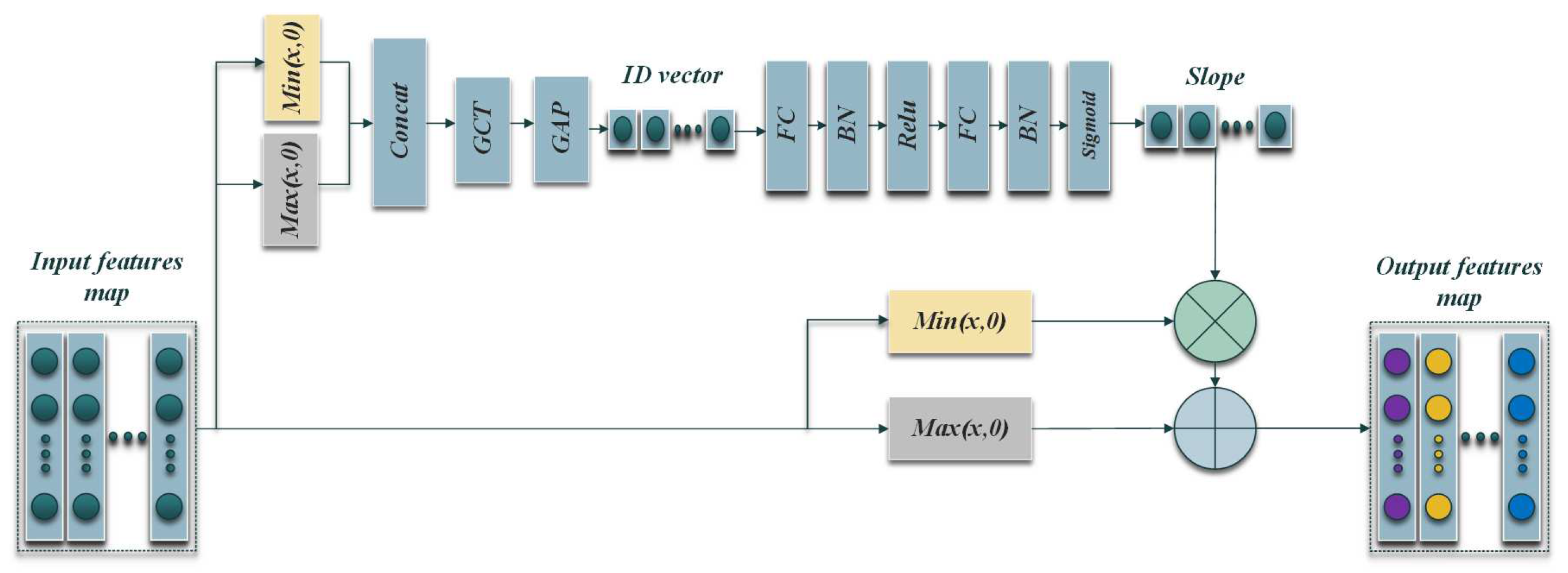
The structure of adaptive activation functions are shown in Figure 4. The input of the subnetwork is concatenated by the one-dimensional vector obtained from the two inputs. The two inputs are positive features after separation and negative features after separation. The separation of positive and negative features can highlight the key features. The following calculation paths are GCT→GAP→FC→ Batch Nomoalation(BN)→ ReLU→ FC→ BN→ Sigmoid →Scales. The function of each layer is described in following section.

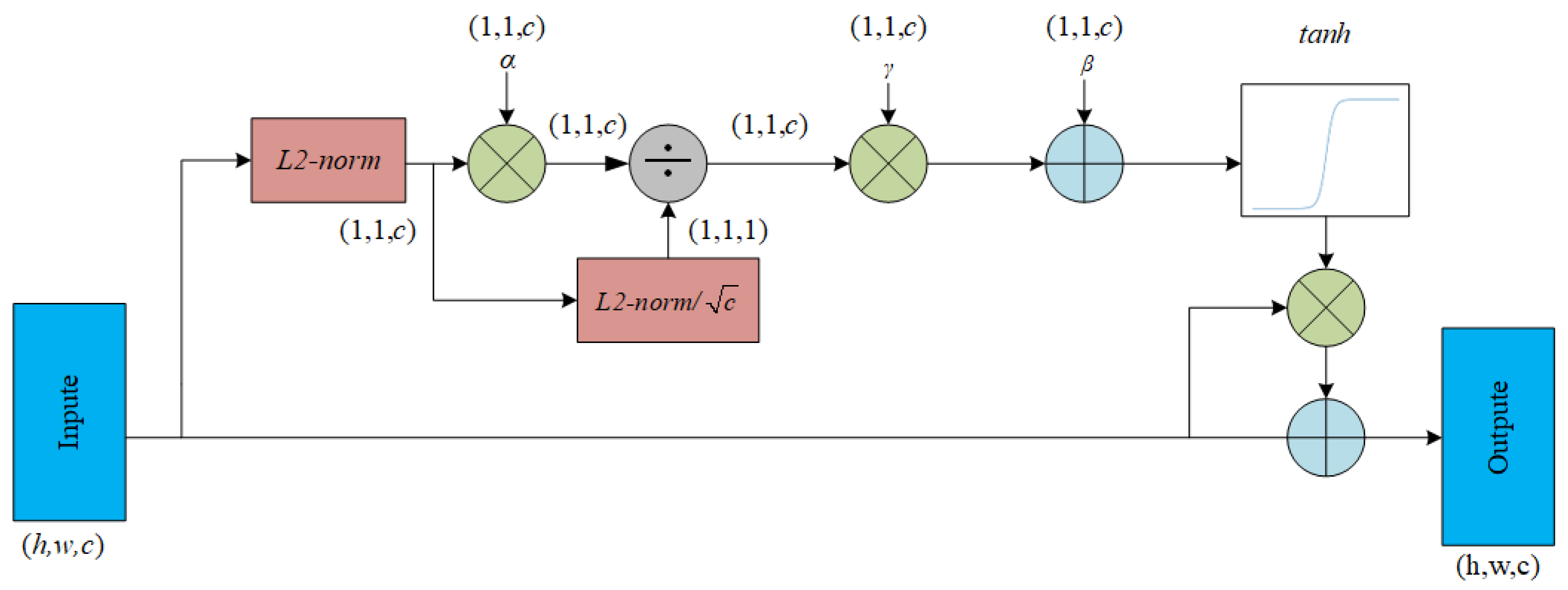
GCT combines normalization methods and attention mechanisms, which makes it easy to analyze the relationships (competition orcooperation) between channels. As shown in Figure 5, The GCT module introduces three trainable parameters

α

β

and

γ

to evaluate the communication channels. Among them,

α

helps embed the output adaptive ability, while

β

and

γ

are used to control the activation threshold, which determines the behavior of GCT in each channel. h and w are the dimensions of feature vectors, c is the number of channals, and L2-norm is the normalization of L2.

Global average pooling (GAP) can replace the fully connected (FC) layer to achieve dimensionality reduction. Eespically, it retains the spatial information extracted from the previous convolutional layers and pooling layers and can also strengthen the relationship between categories and feature maps [27].

ReLU is selected as the activation function of FC in the first layer to reduce the computational complexity and keep the gradient value within a reasonable range for feature extraction. The formula is as follows:

f (x) = \{\begin{matrix} x, x \geq 0 \\ 0, x < 0 \end{matrix}

(4)

Then we add BN layer, which is a way to unify the scattered data and is similar to normal data standardization. It is also a way to optimize the neural network. The data with unified specifications can make it easier to learn the rules in the data for the deep learning model [28] and can also solve the problem of vanishing gradient. The normalization is described by the following formula:

μ = \frac{1}{N_{b a t c h}} \sum_{i = 1}^{N_{b a t c h}} x_{i}

(5)

σ^{2} = \frac{1}{N_{b a t c h}} \sum_{i = 1}^{N_{b a t c h}} (x_{i} - μ)^{2}

(6)

x_{i}^{\land} = \frac{x_{i} - μ}{\sqrt{σ^{2} + ε}}

(7)

y_{i} = ψ x_{i}^{\land} + θ

(8)

where

x_{i}

and

y_{i}

are the observed input and output of each Nbatch,

μ

represents the mean of the input,

σ^{2}

represents the variance of the input,

ε

is a constant near zero, and

θ

ψ

are learnable parameters governing the scaling and shifting distributions. The activation function of the second FC layer is Sigmoid, which can limit the output value during the interval (0,1) and prevent excessive slope from affecting the performance of the activation function.

To summarize the above contents, the proposed adaptive activation function has the ability to automatically learn complex features. Different nonlinear transformation is applied to different inputs to improve the generalization performance of deep learning model, which will well solve the problems in extracting feature contour of indicator diagram and sparsity of indicator diagram in pumping unit fault diagnosis. The following experimental simulation will verify the effectiveness of the designed adaptive activation function.

4. Experimental simulation

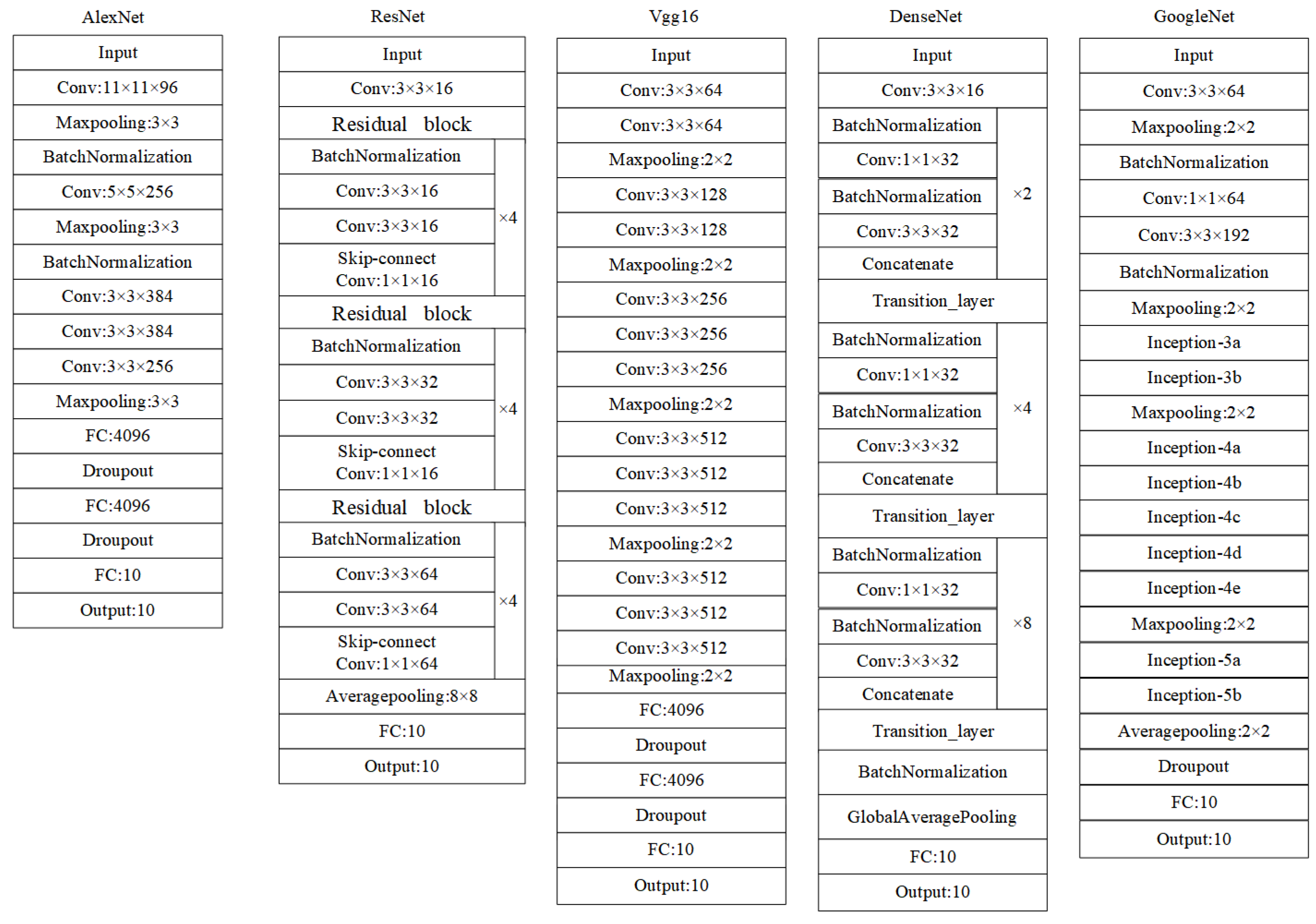
This section mainly verified the performance of our activation function which was tested on AlexNet[20], VGG-16[21], GoogleNet [22], ResNet [23] and DenseNet [24]. The structure diagrams of these five networks are shown in Figure 6. Moreover, we compared our activation function with the traditional activation functions such as ReLU, Sigmoid, Tanh, LReLU and PReLU.

The experiment is mainly divided into two parts. The first part is the simulation on the fault diagnosis dataset of pumping unit. This will prove that the proposed adaptive activation function can extract the features of the indicator diagram and solve the sparsity problem of the indicator diagrams. The improvement in fault diagnosis accuracy indicates that indistinguishable samples are correctly classified. The second part is to verify the superiority of the designed adaptive activation function on the public dataset CIFAR10.

4.1. The dataset of pumping

Adaptive Moment Estimation (Adam) was used here, and the initial learning rate was 0.001. The epoch of training was no less than 200. The average accuracy of each model is shown in Table 1. In the fault diagnosis data set of pumping unit, the adaptive activation function proposed in this paper has the greatest accuracy improvement in the ResNet model. Compared to traditional activation function ReLU, Tanh, Sigmoid, LeakReLU, PReLU, Mish, Swish, the average accuracy of ResNet model with our activation function respectively increased by 1.7%, 5.09%, 5.72%, 2.54%, 1.46%, 1.75%, 1.56%.

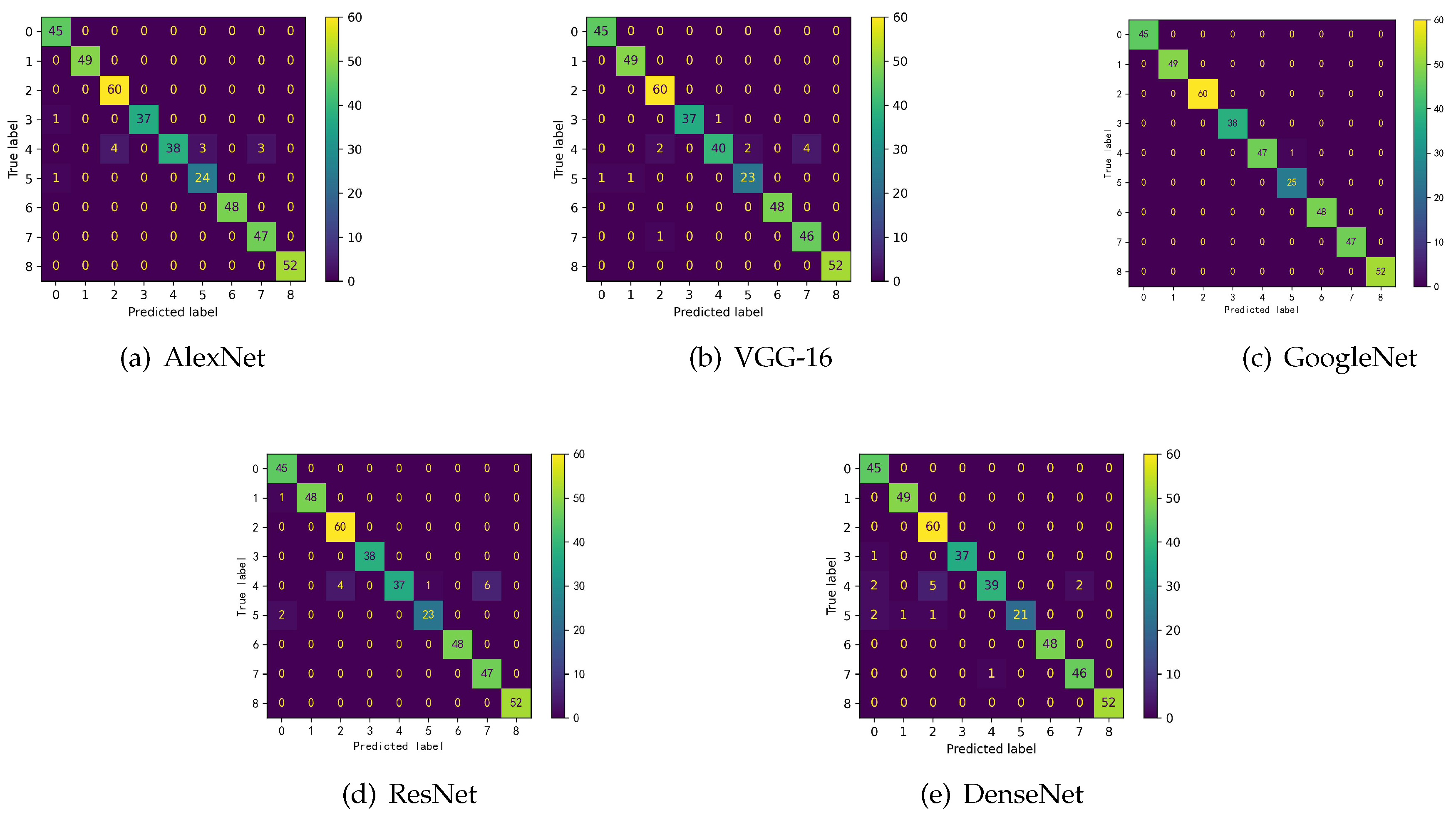
Confusion matrix is a common index and visualization tool to evaluate the results of the classification model and it can judge the advantages and disadvantages of classifiers. The rows of the matrix represent the true value, and the columns of the matrix represent the predicted value. The confusion matrix can respectively count the number of the wrong classification and the right classification, and then display the results in a matrix. Figure 7 shows the confusion matrix of the five models for the pumping unit fault data set. It can be seen that the designed adaptive activation function can effectively represent the mapping relationship between the displacement and the load in the indicator diagram, and extract the features of the indicator diagram, thus those indistinguishable samples are correctly classified. Table 2 gives the accuracy of various types of faults for the five models, which proves that the proposed adaptive activation function can be well applied in the five models and has great adaptability to the models.

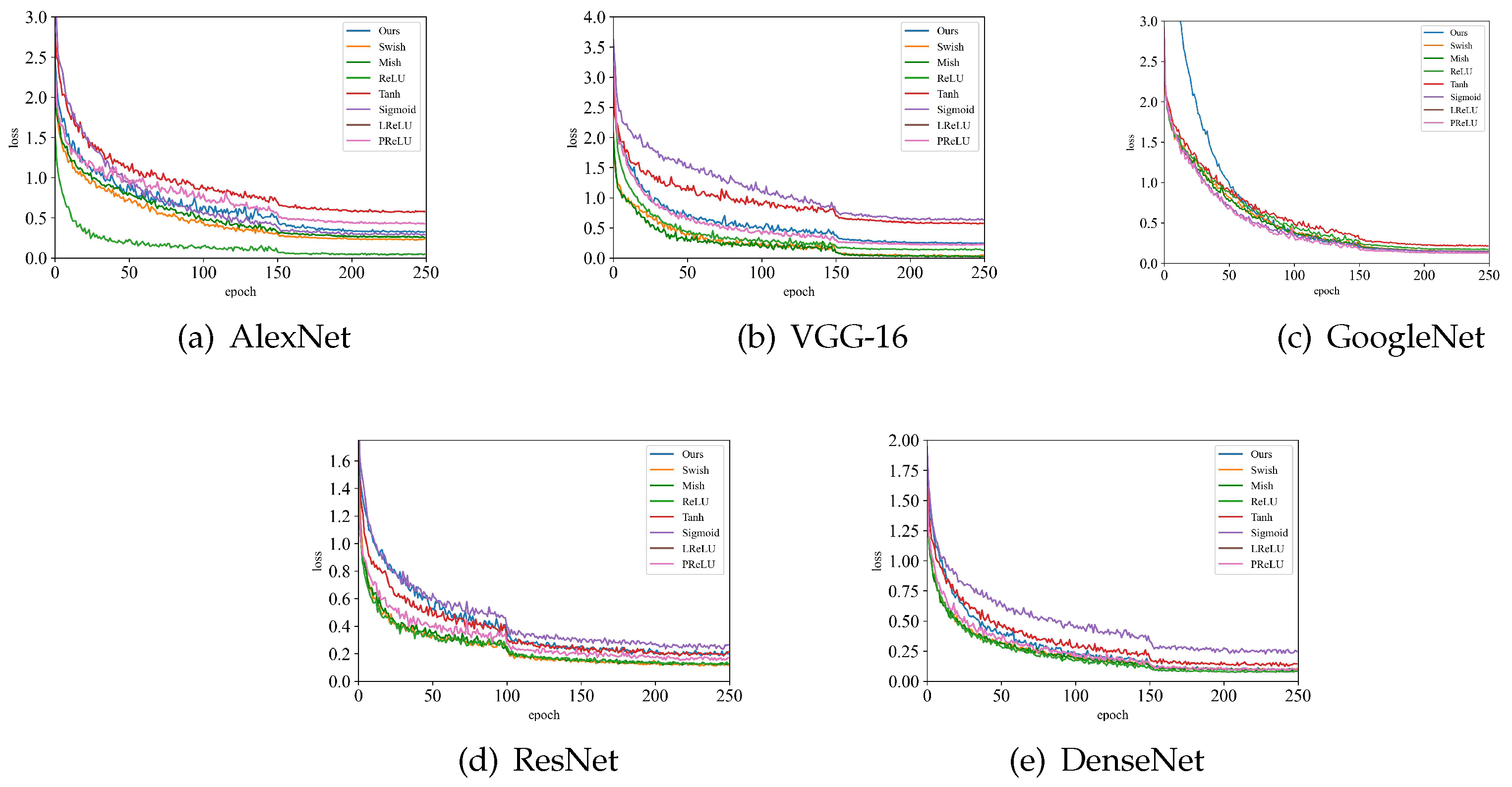
The loss function curve is shown in Figure 8. Among them, (a) AlexNet, (b) VGG-16 and (e) DenseNet have fast convergence speed. The loss functions of (d) ResNet and (e) GoogleNet decline relatively slowly, but eventually converge to the optimal value.

4.2. CIFAR10

We used CIFAR10 data set to conduct experiments and analysed AlexNet, VGG-16, GoogleNet, ResNet and DenseNet models with our activation function and the traditional activation functions. We augmented the data to reduce overfitting. The Adam was used with the initial learning rate 0.001. The epoch of training was no less than 200. The average accuracy of each model is shown in Table 3, where the designed activation function improves the performances of those. Among them, AlexNet, VGG-16 and DenseNet have the best performance. Compared with the traditional activation functions ReLU, Tanh, Sigmoid, LeakReLU, PReLU, Swish, and Mish, our activation function in AlexNet model is improved respectively by 1.84%, 4.11%, 5.45%, 0.79%, 2.74%, 1.91%, 2.04%; our activation function in VGG-16 model is improved respectively by 3.1%, 4.54%, 4.45%, 0.48%, 2.02%, 4.69%, 3.94%; our activation function in DenseNet model is improved respectively by 1.88%, 5.1%, 9.63%, 1.07%, 0.61%, 0.35%, 0.37%. The above data indicate the superiority of the proposed activation function.

5. Conclusions

In this paper, a new adaptive activation function is designed and applied to five models of neural networks. Specifically, the adaptive activation function improves the negative semi-axis slope of the ReLU activation function by combining the gated channel conversion unit to enhance the performance of the deep learning model. The activation function in each layer of neural network is unique, thus the input signal of each layer has a unique nonlinear transformation. Therefore, compared with the traditional fixed activation function, our activation function has a better nonlinear transformation ability and it can be well embedded in five models. Such as through the fault diagnosis data set of pumping unit, it is proved that our activation function can effectively display the mapping relationship between displacement and load in the indicator diagram, thus extract the features of the indicator diagram and solve the sparsity problem of the indicator diagrams. Indistinguishable samples are correctly classified. Through CIFIAR10 dataset, it verifies the superiority and universality of our adaptive activation function.

In short, the proposed adaptive activation function increases the accuracy of fault diagnosis and has a better generalization performance and search ability. Moreover, the proposed adaptive activation functions also can be well embedded in other models of neural networks.

Author Contributions

Conceptualization, Yebin Li and Fangfang Zhang; Funding acquisition, Dongri Shan; Validation, Dongri Shan and Fengying Ma; Resources, Yuanhong Liu; Data Curation, Yebin Li ; Writing—original draft, Yebin Li ; Writing—review & editing, Fangfang Zhang; All authors have read and agreed to the published version of the manuscript.

Funding

This work is supported by the Project of Shandong Provincial Major Scientific and Technological Innovation(Nos.2019JZZY010444, 2019TSLH0315), the Project of 20 Policies of Facilitate Scientific Research in Jinan Colleges (No.2019GXRC063)and the industry-university-research collaborative innovation fund project of Qilu University of Technology (Shandong Academy of Sciences) (Nos.2021CXY-13, 2021CXY-14).

Institutional Review Board Statement

Studies not involving humans or animals.

Data Availability Statement

Not applicable.

Conflicts of Interest

The authors declare no conflict of interest.

References

J. Du, a. K. S. J. Du, a. K. S. Zhigang Liu, and E. Yang, Fault diagnosis of pumping machine based on convolutional neural network, Journal of University of Electronic Science and Technology of China (2020), 751-757.
Gao, Z.; Cecati, C.; Ding, S.X. A Survey of Fault Diagnosis and Fault-Tolerant Techniques—Part I: Fault Diagnosis With Model-Based and Signal-Based Approaches. IEEE Trans. Ind. Electron. 2015, 62, 3757–3767. [Google Scholar] [CrossRef]
Gao, Z.; Cecati, C.; Ding, S.X. A Survey of Fault Diagnosis and Fault-Tolerant Techniques Part II: Fault Diagnosis with Knowledge-Based and Hybrid/Active Approaches. IEEE Trans. Ind. Electron. 2015, 62, 1–1. [Google Scholar] [CrossRef]
Tang, A.; Zhao, W. A Fault Diagnosis Method for Drilling Pump Fluid Ends Based on Time–Frequency Transforms. Processes 2023, 11, 1996. [Google Scholar] [CrossRef]
Fu, Z.; Zhou, Z.; Yuan, Y. Fault Diagnosis of Wind Turbine Main Bearing in the Condition of Noise Based on Generative Adversarial Network. Processes 2022, 10, 2006. [Google Scholar] [CrossRef]
Agarwal, P.; Gonzalez, J.I.M.; Elkamel, A.; Budman, H. Hierarchical Deep LSTM for Fault Detection and Diagnosis for a Chemical Process. Processes 2022, 10, 2557. [Google Scholar] [CrossRef]
Xu, G.; Liu, M.; Jiang, Z.; Shen, W.; Huang, C. Online Fault Diagnosis Method Based on Transfer Convolutional Neural Networks. IEEE Trans. Instrum. Meas. 2019, 69, 509–520. [Google Scholar] [CrossRef]
Y. Duan et al., Improved alexnet model and its application in well dynamogram classification, Computer Applications and Software (2018), 226-230+272.
Sang, J. Research on pump fault diagnosis based on pso-bp neural network algorithm. 2019, 1748–1752. [CrossRef]
Zhang, L.; Du, Q.; Liu, T.; Li, J. A Fault Diagnosis Model of Pumping Unit Based on BP Neural Network. 2020, 454–458. [CrossRef]
Hu, H.; Li, M.; Dang, C. Research on the fault identification method of oil pumping unit based on residual network. 2022, 940–943. [CrossRef]
Bai, T.; Li, X.; Ding, S. Research on Electrical Parameter Fault Diagnosis Method of Oil Well Based on TSC-DCGAN Deep Learning. 2022, 753–761. [CrossRef]
V. Nair and G. E. Hinton, Rectified linear units improve restricted boltzmann machines, International Conference on Machine Learning.
L. Maas, Rectifier nonlinearities improve neural network acoustic models.
He, K.; Zhang, X.; Ren, S.; Sun, J. Delving deep into rectifiers: Surpassing human-level performance on imagenet classification. In Proceedings of the International Conference on Computer Vision, Las Condes, Chile, 11–18 December 2015; pp. 1026–1034. [Google Scholar]
P. Ramachandran, B. P. Ramachandran, B. Zoph, and Q. V. Le, Swish: a self-gated activation function, arXiv: Neural and Evolutionary Computing (2017).
Hu, H.; Liu, A.; Guan, Q.; Qian, H.; Li, X.; Chen, S.; Zhou, Q. Adaptively Customizing Activation Functions for Various Layers. IEEE Trans. Neural Networks Learn. Syst. 2022, 34, 6096–6107. [Google Scholar] [CrossRef] [PubMed]
Zhao, M.; Zhong, S.; Fu, X.; Tang, B.; Dong, S.; Pecht, M. Deep Residual Networks With Adaptively Parametric Rectifier Linear Units for Fault Diagnosis. IEEE Trans. Ind. Electron. 2020, 68, 2587–2597. [Google Scholar] [CrossRef]
Yang, Z.; Zhu, L.; Wu, Y.; Yang, Y. Gated Channel Transformation for Visual Recognition. 2020, 11791–11800. [CrossRef]
Krizhevsky, A.; Sutskever, I.; Hinton, G.E. Imagenet classification with deep convolutional neural networks. Advances in neural information processing systems 2012, 25, 1097–1105. [Google Scholar] [CrossRef]
K. Simonyan and A. Zisserman, Very deep convolutional networks for large-scale image recognition, (2015).
C. Szegedy et al., Going deeper with convolutions, 2015 IEEE Conference on Computer Vision and Pattern Recognition (CVPR) (2014), 1–9.
K. He et al., Deep residual learning for image recognition, 2016 IEEE Conference on Computer Vision and Pattern Recognition (CVPR) (2015), 770–778.
G. Huang, Z. G. Huang, Z. Liu, and K. Q.Weinberger, Densely connected convolutional networks, 2017 IEEE Conference on Computer Vision and Pattern Recognition (CVPR) (2016), 2261–2269.
Cao, L.; Zhao, T. Pumping Unit Design and Control Research. 2019, 1738–1743. [CrossRef]
D. Misra, Mish: A self regularized non-monotonic neural activation function, ArXiv abs/1908.08681 (2019).
M. Lin, Q. Chen, and S. Yan, Network in network, ArXiv abs/1312.4400 (2013).
S. Ioffe and C. Szegedy, Batch normalization: Accelerating deep network training by reducing internal covariate shift, ArXiv abs/1502.03167 (2015).

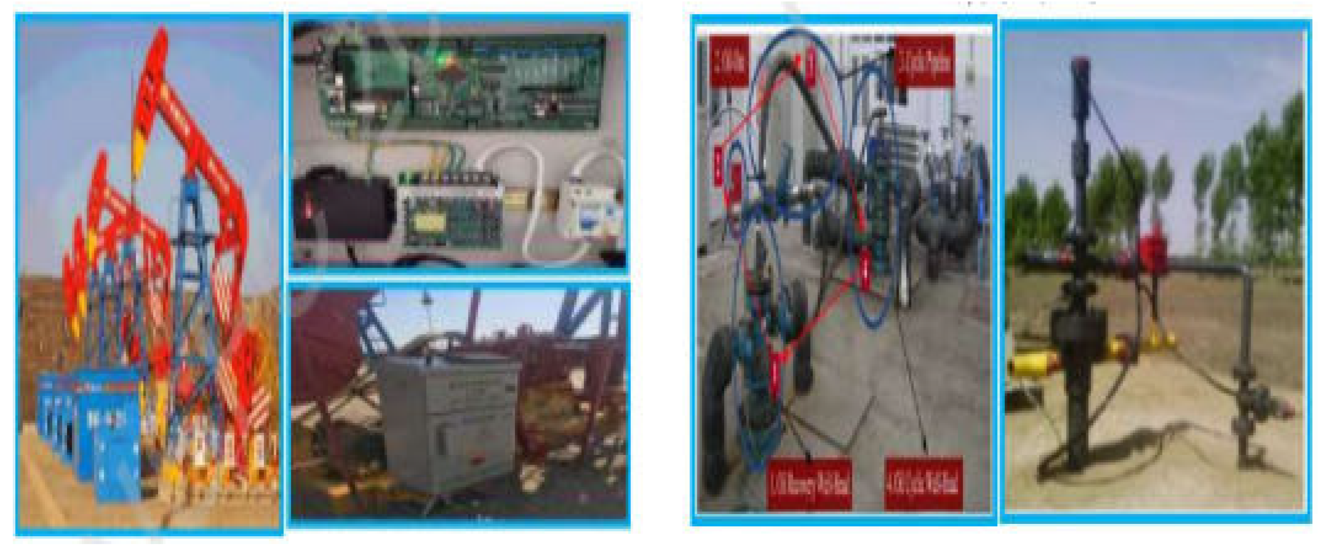
Figure 1. Pumping machine equipment

Figure 2. The operation of the pumping unit.

Figure 3. Fault diagnosis flow chart of pumping unit

Figure 4. Graph of adaptive activation functions

Figure 5. GCT structure drawing

Figure 6. Network architectures of AlexNet,VGG-16,GoogleNet,ResNet, DenseNet

Figure 7. The confusion matrix of the five models of the pumping unit fault diagnosis dataset.

Figure 8. The decline curve of the loss function.

Table 1. CLASSIFICATION PRECISION OF VARIOUS ACTIVATION FUNCTIONS FOR DIFFERENT MODELS ON PUMPING MACHINE FAULT DIAGNOSIS

Methods	AlexNet(%)	VGG-16(%)	GoogleNet(%)	ResNet(%)	DenseNet(%)
Ours	97.91±0.4997	97.57±0.2658	99.13±0.1941	97.82±0.4061	97.52±0.4706
ReLU	97.33±0.5534	96.94±0.9537	98.56±0.3220	96.12±0.6140	96.89±0.0970
Sigmoid	94.51±0.4930	96.41±0.3567	96.17±0.2831	92.14±0.2145	94.17±0.6584
Tanh	96.41±0.3220	97.04±0.4706	97.91±0.3632	94.66±0.3070	95.05±0.4231
LReLU	97.48±0.8209	97.14±0.5405	98.74±0.2830	95.28±0.9029	96.36±0.5091
PReLU	97.43±0.6254	97.04±0.3220	98.74±0.6584	96.36±0.5091	97.04±0.3883
Mish	97.23±0.6063	96.02±0.6254	98.74±0.2830	96.07±0.3883	97.17±0.1144
Swish	97.72±0.3292	95.15±0.8547	98.74±0.1816	96.26±0.3943	96.75±0.5661

Table 2. DIAGNOSTIC ACCURACY OF FIVE MODELS FOR EACH FAULT TYPE OF PUMPING UNIT

The type of fault	AlexNet	VGG-16	GoogleNet	ResNet	DenseNet
Pump up touch	0.96	0.98	0.90	0.96	0.90
Pumping rod detachment	1.00	0.98	0.96	0.98	1.00
Insufficient liquid supply	0.94	0.95	0.93	0.95	0.91
Contain sand	1.00	1.00	1.00	1.00	1.00
Piston stuck	1.00	0.98	0.98	1.00	0.97
Gas influence	0.89	0.92	0.98	0.92	1.00
Double valve leakage	1.00	1.00	1.00	1.00	1.00
Pump down touch	0.94	0.92	0.93	0.90	0.96
Normal	1.00	1.00	1.00	1.00	1.00

Table 3. CLASSIFICATION PRECISION OF VARIOUS ACTIVATION FUNCTIONS FOR DIFFERENT MODELS ON CIFAR10

Methods	AlexNet(%)	VGG-16(%)	GoogleNet(%)	ResNet(%)	DenseNet(%)
Ours	91.10±0.0445	93.86±0.0406	90.35±0.1070	91.73±0.0231	92.30±0.0681
ReLU	89.26±0.0576	90.76±0.0987	89.00±0.0337	90.27±0.0034	90.42±0.0846
Sigmoid	85.65±0.0365	89.32±0.1127	87.23±0.0485	88.06±0.0835	82.67±0.2110
Tanh	86.99±0.2432	89.41±0.0189	83.69±0.0402	88.68±0.0414	87.20±0.0745
LReLU	90.31±0.2147	93.38±0.0414	89.70±0.0527	91.24±0.1059	91.23±0.0684
PReLU	88.36±0.0436	91.84±0.0633	89.31±0.0454	91.08±0.0637	91.69±0.0755
Mish	89.07±0.0847	89.92±0.0577	88.64±0.0729	91.12±0.7960	91.97±0.0758
Swish	89.19±0.0628	89.19±0.0618	88.94±0.1161	90.93±0.0850	91.95±0.0893

Disclaimer/Publisher’s Note: The statements, opinions and data contained in all publications are solely those of the individual author(s) and contributor(s) and not of MDPI and/or the editor(s). MDPI and/or the editor(s) disclaim responsibility for any injury to people or property resulting from any ideas, methods, instructions or products referred to in the content.

© 2023 by the authors. Licensee MDPI, Basel, Switzerland. This article is an open access article distributed under the terms and conditions of the Creative Commons Attribution (CC BY) license (http://creativecommons.org/licenses/by/4.0/).

Copyright: This open access article is published under a Creative Commons CC BY 4.0 license, which permit the free download, distribution, and reuse, provided that the author and preprint are cited in any reuse.

MDPI Initiatives

Important Links

Choose an area of interest and we will send you notifications of new preprints at your preferred frequency.

Disclaimer