Preprint
Article

Square Root Statistics of Density Matrices and Their Applications

Altmetrics

Downloads

160

Views

64

Comments

0

A peer-reviewed article of this preprint also exists.

This version is not peer-reviewed

Submitted:

10 August 2023

Posted:

10 August 2023

You are already at the latest version

Alerts
Abstract
To estimate the degree of quantum entanglement, it is important to understand the statistical behavior of functions of spectrum of density matrices such as von Neumann entropy, quantum purity, and entanglement capacity. These entangle- ment metrics over different generic state ensembles have been studied intensively in the literature. As an alternative metric, in this work we study sum of square root spectrum of density matrices, which is relevant to negativity and fidelity in quantum information processing. In particular, we derive the exact mean and vari- ance of sum of square root spectrum over the Bures-Hall generic state ensemble extending known results obtained recently over the Hilbert-Schmidt ensemble.
Keywords: 
Subject: Computer Science and Mathematics  -   Probability and Statistics

1. Introduction and Main Results

1.1. Square Root Spectrum and Applications

The sum of square root of spectrum of density matrices is defined as
Λ = i = 1 m λ i 1 2 ,
where m is the dimension of the density matrix and the set { λ i } i = 1 m is its spectrum. The random variable (1) is closely related to the negativity (2) and fidelity (3) as discussed below.
Negativity is introduced in [1] as a computable measure of entanglement. For a pure state ρ = ψ ψ with ψ = j = 1 m λ j j j and j = 1 m λ j = 1 , the negativity is defined as
N ( ρ ) = | | ρ T A | | 1 1 2 = j k λ j λ k 2 = j = 1 m λ j 2 1 2 = Λ 2 1 2 ,
where | | · | | 1 is the trace norm (also known as the Schatten 1-norm) and ρ T A refers to the partial transpose of ρ . Moreover, it has a uniqueness property that suppose E ( ρ ) is a weak entanglement monotone that is a symmetric function of negative eigenvalues of ρ T A , then E ( ρ ) is a nondecreasing function of N ( ρ ) , and E ( ρ ) = c log ( 1 + 2 N ( ρ ) ) for some constant c 0 in the case that it is additive, see [2].
Fidelity [3] refers to a measure of the similarity or overlap between two quantum states. It quantifies how closely one quantum state resembles another. It is defined as:
F ( σ , ρ ) = tr σ ρ σ 2 .
In this work, we only consider the case that σ = 1 m I m , which is the maximum mixed state, and ρ is the the density matrix corresponding to Bures-Hall ensemble. In this case, we have
F ( σ , ρ ) = 1 m Λ 2 .
The case of Hilbert-Schmidt is computed in [4].

1.2. Description of Bures-Hall Ensemble

The Bures-Hall ensemble is described as follows [5,6]. Consider a composite(bipartite) system that consists of two subsystems A and B of Hilbert space(complex vector space) with dimensions m and n, respectively. The Hilbert space H A + B = H A H B . A random pure state of the composite system H A + B is defined as a linear combination of the random coefficients z i , j and the complete basis i A and j B of H A and H B [5],
ψ = i = 1 m j = 1 n z i , j i A j B ,
where each z i , j follows the standard Gaussian distribution. We now consider a superposition of the state (5),
φ = ψ + ( U I m ) ψ ,
where U is an m × m unitary random matrix with the measure proportional to det ( I m + U ) 2 α + 1 [7]. The corresponding density matrix of the pure state (6) is
ρ = φ φ ,
which has the natural probability constraint
tr ( ρ ) = 1 .
Without loss of generality, we assume that m n . The reduced density matrix ρ A of the smaller subsystem A is computed by partial tracing (purification) of the full density matrix (7) over the other subsystem B (environment) as
ρ A = tr B ρ .
The resulting density of the eigenvalues of ρ A ( λ i [ 0 , 1 ] , i = 1 , . . . , m ) is the (generalized) complex Bures-Hall measure [7,8,9,10],
f ( λ ) = 1 C δ 1 i = 1 m λ i 1 i < j m ( λ i λ j ) 2 λ i + λ j i = 1 m λ i α ,
where the parameter α takes half-integer values,
α = n m 1 2 ,
and the constant C is
C = 2 m ( m + 2 α ) π m / 2 Γ ( m ( m + 2 α + 1 ) / 2 ) i = 1 m Γ ( i + 1 ) Γ ( i + 2 α + 1 ) i + α + 1 2 .
For convenience, we need to define the random variable below:
Λ = i = 1 m λ i 1 2 , Λ [ 1 , m ] .
Then, the negativity and fidelity are defined, respectively, as
N = 1 2 Λ 2 1 , F = F ( σ , ρ ) = 1 m Λ 2 .

1.3. Main Results

Proposition 1.1 The exact mean of the random variable Λ defined in (13) valid for any subsystem dimensions m n under the Bures-Hall ensemble (10) is obtained as
E f [ Λ ] = Γ ( d ) Γ ( d + 1 2 ) π k = 0 m 1 Γ ( k + 2 α + m + 2 ) Γ ( m k 1 2 ) Γ ( k + 3 2 ) Γ ( k + 2 α + m + 5 2 ) Γ ( m k ) Γ ( k + 1 ) × Γ ( k + 2 α + 5 2 ) Γ ( k + α + 5 2 ) Γ ( k + 2 α + 2 ) Γ ( k + α + 2 ) 1 + k + α + 1 k + α + 3 2 ,
where d is
d = 1 2 m ( m + 2 α + 1 ) .
The proof of Proposition 1.1 is given in Sec. 2.2.
Proposition 1.2 The exact second moment of Λ in (13) valid for any subsystem dimensions m n under the Bures-Hall ensemble (10) is obtained as
E f [ Λ 2 ] = 1 2 d k = 0 m 1 ( ( 1 ) k + m Γ ( k + 2 α + m + 2 ) Γ ( k + 2 ) Γ ( k + 2 α + 2 ) Γ ( k + 2 α + 2 α ) Γ ( m k ) k ! + ( 1 ) k + m Γ ( k + 1 + 2 α + 2 ) Γ ( k + 1 + 2 α + 2 α ) Γ ( k + 1 + 2 α + m + 2 ) Γ ( k + 1 m + 1 ) ) + 1 4 π 2 d k = 0 m 1 j = 0 m 1 l k , 0 l j , 0 l k , 1 2 l j , 1 2 ( 4 2 + 1 2 ( j + α + 1 ) 2 + 1 2 ( k + α + 1 ) 2 1 k j 1 2 1 j k 1 2 1 + j + α + 3 2 j + α + 1 k + α + 3 2 k + α + 1 + 4 3 2 + j + α ( 2 + j + k + 2 α ) ( 3 + j + k + 2 α ) ( 1 + α + j ) ) ,
where we denote
l k , β = Γ ( m + 2 α + k + 2 + β ) Γ ( k + 1 + β ) Γ ( k + α + 1 + β ) Γ ( k + 2 α + 2 + β ) Γ ( m k β ) .
Therefore, the mean of negativity and fidelity, valid for any subsystem dimensions m n , are obtained, respectively, as
E f [ N ] = 1 2 E f [ Λ 2 ] 1 , E f [ F ] = 1 m E f [ Λ 2 ] ,
where the expectation E f [ . ] is taken over the Bures-Hall ensemble (10). The exact variance of the first moment Λ under the Bures-Hall ensemble is given by
V f [ Λ ] = E f [ Λ 2 ] E f 2 [ Λ ] .
The proof of these results is given in Sec. 2.3.
Now we can understand the distribution of the Λ with the expressions of the mean (15) and variance (20). For convenience, we standardize Λ as
X = Λ E f [ Λ ] V f [ Λ ] ,
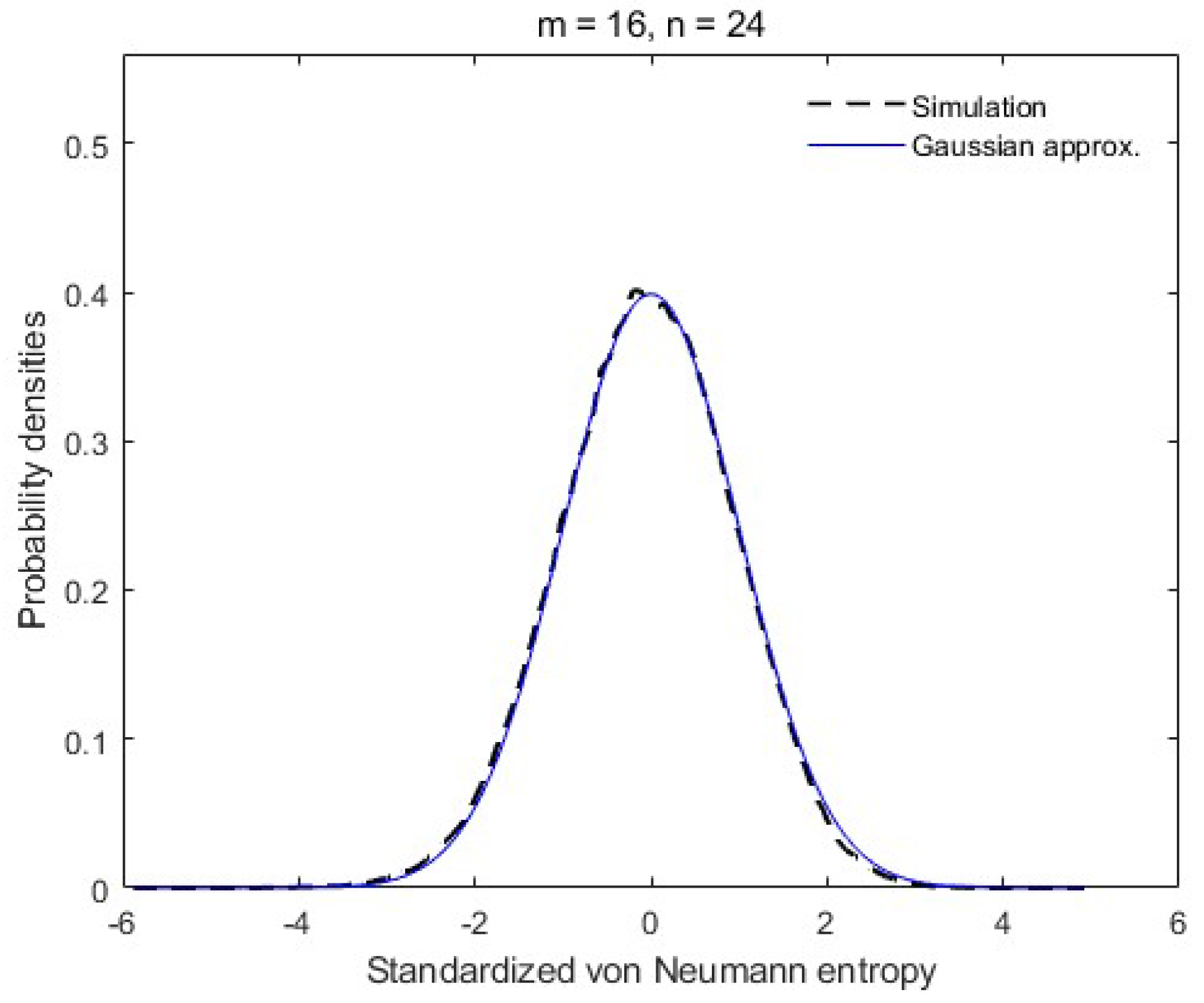
which make the random variable X be supported in X ( , ) with zero mean and unit variance. We obtain the simulation with comparison to Gaussian distribution by Matlab.
As we can see from the Figure 1 and Figure 2, while the distribution of von Neumann entropy which is conjectured to be the same as Gaussian distribution [11,12], the distribution of Λ is also similar to Gaussian distribution.

2. Computing Moments of Sum of Square Root Statistics

2.1. Ensemble Conversion

We calculate the random variables under the original ensemble by covering it to unconstrained ensemble. The unconstrained ensemble of the Bures-Hall measure is
h ( x ) = 1 C 1 i < j m ( x i x j ) 2 x i + x j i = 1 m x i α e x i
where x i [ 0 , ) , i=1,...,m, and the constant C’ depends on the constant (12) as
C = C Γ ( d )
with d denoting
d = 1 2 m ( m + 2 α + 1 )
The density of trace
θ = i = 1 m x i , θ [ 0 , )
is obtained as
g ( θ ) = x h ( x ) δ θ i = 1 m x i i = 1 m d x i = C C e θ θ d 1 λ f ( λ ) d λ i = 1 Γ ( d ) e θ θ d 1 ,
where we have applied the change of variables
x i = θ λ i ,
implies that h ( x ) is factored as [13]
h ( x ) i = 1 m d x i = f ( λ ) g ( θ ) d θ i = 1 m d λ i
which shows θ is independent of each λ i .
By multiplying an appropriate constant (26),
1 = 0 1 Γ ( d + 1 ) e θ θ d d θ ,
denote that
Λ = i = 1 m λ i 1 2 X = i = 1 m x i 1 2 ,
we have
E f [ Λ ] = 0 e θ θ d 1 2 Γ ( d + 1 2 ) d θ 0 Λ f ( λ ) i = 1 m d λ i = 0 0 X θ 1 2 e θ θ d 1 2 Γ ( d + 1 2 ) f ( λ ) d θ i = 1 m d λ i = Γ ( d ) Γ ( d + 1 2 ) 0 e θ θ d 1 Γ ( d ) d θ 0 X f ( λ ) i = 1 m d λ i = Γ ( d ) Γ ( d + 1 2 ) 0 X h ( x ) i = 1 m d x i = Γ ( d ) Γ ( d + 1 2 ) E h [ X ] .
The variance is defined as
V f [ Λ ] = E f Λ E f [ Λ ] 2 = E f [ Λ 2 ] E f 2 [ Λ ] .
We have
E f [ Λ 2 ] = 0 Λ 2 f ( λ ) i = 1 m d λ i = 0 0 X 2 1 θ f ( λ ) d θ i = 1 m d λ i .
Similarly, by multiplying a proper constant (29), we obtain
E f [ Λ 2 ] = Γ ( d ) Γ ( d + 1 ) E h [ X 2 ] .
Applying (31) and (34), we have
V f [ Λ ] = 1 d E h [ X 2 ] Γ ( d ) Γ ( d + 1 2 ) 2 E h 2 [ X ] .

2.2. Calculation of the Mean of Λ

Following the formulas for E h [ T P ] [14, Eq. (26) to (48)], with the same notation, letting
I q ( β ) = k = 0 m 1 ( 1 ) k Γ ( k + 2 α + m + 2 ) Γ ( m k β ) Γ ( k + 2 α + 2 ) Γ ( k + 2 α + 2 q ) Γ ( m k ) k ! Γ ( k + β + 2 α + 2 ) Γ ( k + β + 2 α + 2 q ) Γ ( k + β + 2 α + m + 2 ) Γ ( k β ) ,
letting β = 1 2 instead of β = 2 , we obtain
E h [ X ] = 1 2 0 x 1 2 1 G α ( x ) + G α + 1 ( x ) d t d x = 1 2 1 0 x 1 2 G α ( x ) + G α + 1 ( x ) d x d t = 1 2 1 t 3 2 ( I α β + I α + 1 β ) d t = k = 0 m 1 ( 1 ) k Γ ( k + 2 α + m + 2 ) Γ ( m k 1 2 ) Γ ( k + 2 α + 2 ) Γ ( k + α + 2 ) Γ ( m k ) k ! Γ ( k + 1 2 + 2 α + 2 ) Γ ( k + 1 2 + α + 2 ) Γ ( k + 1 2 + 2 α + m + 2 ) Γ ( k 1 2 ) k = 0 m 1 ( 1 ) k Γ ( k + 2 α + m + 2 ) Γ ( m k 1 2 ) Γ ( k + 2 α + 2 ) Γ ( k + α + 1 ) Γ ( m k ) k ! Γ ( k + 1 2 + 2 α + 2 ) Γ ( k + 1 2 + α + 1 ) Γ ( k + 1 2 + 2 α + m + 2 ) Γ ( k 1 2 )
Applying the identity of Gamma function:
Γ 1 2 k = ( 1 ) k 1 Γ ( 1 2 ) Γ ( 1 2 ) Γ ( k + 1 + 1 2 ) ,
we are able to write the result as
E h [ X ] = 1 π k = 0 m 1 Γ ( k + 2 α + m + 2 ) Γ ( m k 1 2 ) Γ ( k + 3 2 ) Γ ( k + 2 α + m + 5 2 ) Γ ( m k ) Γ ( k + 1 ) Γ ( k + 2 α + 5 2 ) Γ ( k + α + 5 2 ) Γ ( k + 2 α + 2 ) Γ ( k + α + 2 ) × 1 + k + α + 1 k + α + 3 2
Therefore, the mean of Λ is given by
E f [ Λ ] = Γ ( d ) Γ ( d + 1 2 ) π k = 0 m 1 Γ ( k + 2 α + m + 2 ) Γ ( m k 1 2 ) Γ ( k + 3 2 ) Γ ( k + 2 α + m + 5 2 ) Γ ( m k ) Γ ( k + 1 ) Γ ( k + 2 α + 5 2 ) Γ ( k + α + 5 2 ) Γ ( k + 2 α + 2 ) Γ ( k + α + 2 ) × 1 + k + α + 1 k + α + 3 2

2.3. Calculation of the Second Moment

By (35), now it suffices to calculate E h [ X 2 ] .
E h [ X 2 ] = x i = 1 m x i 1 2 2 h ( x ) i = 1 m d x i = x i = 1 m x i h ( x ) i = 1 m d x i + 2 x 1 i < j m x i 1 2 x j 1 2 h ( x ) i = 1 m d x i = m 0 x h 1 ( x ) d x + m ( m 1 ) 0 0 x 1 2 y 1 2 h 2 ( x , y ) d x d y ,
where
h 1 ( x ) = 1 2 m K 01 ( x , x ) + K 10 ( x , x ) h 2 ( x , y ) = 1 4 m ( m 1 ) ( K 01 ( x , x ) + K 10 ( x , x ) K 01 ( y , y ) + K 10 ( y , y ) 2 K 01 ( x , y ) K 01 ( y , x ) 2 K 10 ( x , y ) K 10 ( y , x ) 2 K 00 ( x , y ) K 11 ( x , y ) 2 K 00 ( y , x ) K 11 ( y , x ) ) ,
where
K 00 ( x , y ) = 0 1 t 2 α + 1 H α ( t x ) H α + 1 ( t y ) d t K 01 ( x , y ) = x 2 α + 1 0 1 t 2 α + 1 H α ( t y ) G α + 1 ( t x ) d t K 10 ( x , y ) = y 2 α + 1 0 1 t 2 α + 1 H α + 1 ( t x ) G α ( t y ) d t K 11 ( x , y ) = ( x y ) 2 α + 1 0 1 t 2 α + 1 G α + 1 ( t x ) G α ( t y ) d t x α y α + 1 x + y ,
where we denote
H q ( x ) = G 2 , 3 1 , 1 [ ] m 2 α 1 ; m 0 ; q , 2 α 1 x G q ( x ) = G 2 , 3 2 , 1 [ ] m 2 α 1 ; m 0 , q ; 2 α 1 x .
The kernal functions above((39) and (42) to (44)) are obtained in [15,16] , which were successfully used in calculating the mean and variance of von Neumann entropy under Bures-Hall ensemble [11].
So we can calculate five integrals separately to get the result:
I 1 = 0 x ( K 01 ( x , x ) + K 10 ( x , x ) ) d x I A = 0 x 1 2 ( K 01 ( x , x ) + K 10 ( x , x ) ) d x I B = 0 0 x 1 2 y 1 2 K 01 ( x , y ) K 01 ( y , x ) d x d y I C = 0 0 x 1 2 y 1 2 K 10 ( x , y ) K 10 ( y , x ) d x d y I D = 0 0 x 1 2 y 1 2 K 00 ( x , y ) K 11 ( x , y ) d x d y

2.3.1. Calculation of I 1 and I A

The evaluation of I 1 and I A could also be obtained by the formula for I A [11] with β = 1 and β = 1 2 respectively. Denoting
A q ( t ) = 0 x β ( t x ) 2 α + 1 H 2 α + 1 q ( t x ) G q ( t x ) d x A q ( t ) = t β 1 A q ,
where
A q = k = 0 m 1 ( 1 ) k + m Γ ( k + 2 α + m + 2 ) Γ ( k + β + 1 ) Γ ( k + 2 α + 2 ) Γ ( k + 2 α + 2 q ) Γ ( m k ) k ! Γ ( k + β + 2 α + 2 ) Γ ( k + β + 2 α + 2 q ) Γ ( k + β + 2 α + m + 2 ) Γ ( k + β m + 1 ) .
Notice that when β = 0 , A q = 0 , so we get another expression of K 01 and K 11 :
K 01 ( x , y ) = x 2 α + 1 0 t 2 α + 1 H α ( t x ) G α + 1 ( t y ) d t K 10 ( x , y ) = y 2 α + 1 1 t 2 α + 1 G α ( t x ) H α + 1 ( t y ) d t
By changing the order of integrals, I 1 and I A can be calculated as
I 1 = 0 1 x 1 ( t x ) 2 α + 1 H α ( t x ) G α + 1 ( t x ) + G α ( t x ) H α + 1 ( t x ) d t d x = 1 t 1 1 ( A α + A α + 1 ) d t = ( A α + A α + 1 ) | β = 1 I A = 0 1 x 1 2 ( t x ) 2 α + 1 H α ( t x ) G α + 1 ( t x ) + G α ( t x ) H α + 1 ( t x ) d t d x = 1 t 1 2 1 ( A α + A α + 1 ) d t = 2 ( A α + A α + 1 ) | β = 1 2

2.3.2. Calculation of I B and I C

Calculation of I B and I C follows almost the same procedure. It starts from the fact that the kernels (43) as well as finite sum representation [14,17] of the Meijer G-functions G 2 , 3 1 , 1 . Directly evaluate the integrals over t by the identity [18]
0 1 x a 1 G p , q m , n ( a 1 , , a n ; a n + 1 , , a p b 1 , , b m ; b m + 1 , , b q | η x ) d x = G p + 1 , q + 1 m , n + 1 ( 1 a , a 1 , , a n ; a n + 1 , , a p b 1 , , b m ; b m + 1 , , b q , a | η ) .
This leads I B and I C to
I B = j , k = 0 m 1 f j , k f k , j I C = j , k = 0 m 1 g j , k g k , j
where we denote
f j , k = ( 1 ) j Γ ( m + 2 α + j + 2 ) Γ ( j + 1 ) Γ ( α + j + 1 ) Γ ( 2 α + j + 2 ) Γ ( m j ) 0 x 1 2 G 3 , 4 2 , 2 ( j k , j m ; m + 2 α + j + 1 2 α + j + 1 , α + j ; j , j k 1 | x ) d x
g j , k = ( 1 ) j Γ ( m + 2 α + j + 2 ) Γ ( j + 1 ) Γ ( α + j + 2 ) Γ ( 2 α + j + 2 ) Γ ( m j ) 0 x 1 2 G 3 , 4 2 , 2 ( j k , j m ; m + 2 α + j + 1 2 α + j + 1 , α + j + 1 ; j , j k 1 | x ) d x
As
0 x s 1 G p , q m , n ( a 1 , , a n ; a n + 1 , , a p b 1 , , b m ; b m + 1 , , b q | η x ) d x = η s j = 1 m Γ ( b j + s ) j = 1 n Γ ( 1 a j s ) j = n + 1 p Γ ( a j + s ) j = m + 1 q Γ ( 1 b j s ) ,
we get
f j , k = ( 1 ) j Γ ( m + 2 α + j + 2 ) Γ ( j + 2 α + 1 + 3 2 ) Γ ( j + 1 ) Γ ( α + j + 1 ) Γ ( 2 α + j + 2 ) Γ ( m j ) × Γ ( j + α + 3 2 ) Γ ( 1 j + k 3 2 ) Γ ( 1 j + m 3 2 ) ) Γ ( m + 2 α + j + 5 2 ) Γ ( 1 2 j ) Γ ( 1 2 j + k )
g j , k = f j , k j + α + 3 2 j + α + 1 .
Applying the identity of Gamma function (38), f j , k can be rewritten as
Γ ( m + 2 α + j + 2 ) Γ ( j + 3 2 ) Γ ( m j 1 2 ) Γ ( j + 1 ) Γ ( j + α + 1 ) Γ ( j + 2 α + 2 ) Γ ( m j ) Γ ( j + 2 α + 5 2 ) Γ ( j + α + 3 2 ) Γ ( m + 2 α + j + 5 2 ) ( k j 1 2 ) π .
Define that
l j , x = Γ ( m + 2 α + j + 2 + x ) Γ ( j + 1 + x ) Γ ( j + α + 1 + x ) Γ ( j + 2 α + 2 + x ) Γ ( m j x ) ,
we get
f j , k = 1 π l j , 0 l j , 1 2 1 k j 1 2 .

2.3.3. Calculation of I D

To calculate I D , we use another form of the correlation kernels [18]
K 00 ( x , y ) = k = 0 m 1 2 ( k + α + 1 ) G 2 , 3 1 , 1 ( 2 α 1 k ; k + 1 0 ; α , 2 α 1 | x ) G 2 , 3 1 , 1 ( 2 α 1 k ; k + 1 0 ; α 1 , 2 α 1 | y ) K 11 ( x , y ) = x α y α + 1 k = 0 m 1 2 ( k + α + 1 ) G 2 , 3 2 , 1 ( α k 1 ; α + k + 1 0 , α ; α 1 | y ) G 2 , 3 2 , 1 ( α k ; α + k + 2 0 , α + 1 ; α | x ) x α y α + 1 e x y x + y .
As the function can be factorized, we can calculate them separately
0 x β x α e x p j ( x ) Q k ( x ) d x = ( 1 ) j + k + 1 0 G 2 , 3 1 , 1 ( 2 α 1 j ; j + 1 0 ; α , 2 α 1 | x ) G 2 , 3 2 , 1 ( β k ; β + 2 α + k + 2 β + α , β + 2 α + 1 ; β | x ) d x = ( 1 ) j + k + 1 0 Γ ( 2 α + 2 + j ) Γ ( 1 + α ) Γ ( 2 α + 2 ) Γ ( j + 1 ) 2 F 2 ( 2 α + 2 + j , j ; 1 + α , 2 α + 2 ; x ) G 2 , 3 2 , 1 ( β k ; β + 2 α + k + 2 β + α , β + 2 α + 1 ; β | x ) d x = i = 0 j ( 1 ) i + j + k + 1 Γ ( 2 α + 2 + j + i ) Γ ( 1 + α + i ) Γ ( 2 α + 2 + i ) Γ ( i + 1 ) Γ ( j i + 1 ) 0 x i G 2 , 3 2 , 1 ( β k ; β + 2 α + k + 2 β + α , β + 2 α + 1 ; β | x ) d x = i = 0 j ( 1 ) i + j + 1 Γ ( 2 α + 2 + j + i ) Γ ( β + i + 1 ) Γ ( 1 + α + i ) Γ ( 2 α + 2 + i ) Γ ( i + 1 ) Γ ( j i + 1 ) Γ ( β + α + i + 1 ) Γ ( β + 2 α + i + 2 ) Γ ( β + 2 α + k + i + 3 ) Γ ( β + i + 1 k )
Similarly,
0 y β y α + 1 e y q j ( y ) P k ( y ) d y = s = 0 j ( 1 ) s + j + 1 Γ ( 2 α + 2 + j + s ) Γ ( β + s + 1 ) Γ ( 2 + α + s ) Γ ( 2 α + 2 + s ) Γ ( s + 1 ) Γ ( j s + 1 ) Γ ( β + α + s + 2 ) Γ ( β + 2 α + s + 2 ) Γ ( β + 2 α + k + s + 3 ) Γ ( β + s + 1 k )
While
0 0 x β y β p j ( x ) q j ( y ) x α y α + 1 e x y x + y d x d y = i = 0 j k = 0 j 1 Γ ( i + 1 ) Γ ( j i + 1 ) ( 1 ) k + i Γ ( 2 α + 2 + j + i ) Γ ( 1 + α + i ) Γ ( 2 α + 2 + i ) Γ ( 2 α + 2 + j + k ) Γ ( 2 + α + k ) Γ ( 2 α + 2 + k ) Γ ( k + 1 ) Γ ( j k + 1 ) × Γ ( β + α + i + 1 ) Γ ( β + α + k + 2 ) 2 β + i + k + 2 α + 2
Applying equation (38), with the notation (18) above, we obtain
I D = 1 π 2 i = 0 m 1 j = 0 m 1 l i , 0 l j , 0 l i , 1 2 l j , 1 2 1 2 + α + j + 1 ( 2 + i + j + 2 α ) ( 2 + i + j + 2 α + 1 ) ( 1 + α + j )
Applying the equations (49), (51) and (64) above, we can finally obtain that
E h [ X 2 ] = 1 2 I 1 + 1 4 I A 1 2 ( I B + I C ) I D = 1 2 k = 0 m 1 ( ( 1 ) k + m Γ ( k + 2 α + m + 2 ) Γ ( k + 2 ) Γ ( k + 2 α + 2 ) Γ ( k + α + 2 ) Γ ( m k ) k ! Γ ( k + 2 α + 3 ) Γ ( k + α + 3 ) Γ ( k + 2 α + m + 3 ) Γ ( k m + 2 ) + ( 1 ) k + m Γ ( k + 2 α + m + 2 ) Γ ( k + 2 ) Γ ( k + 2 α + 2 ) Γ ( k + α + 1 ) Γ ( m k ) k ! Γ ( k + 2 α + 3 ) Γ ( k + α + 2 ) Γ ( k + 2 α + m + 3 ) Γ ( k m + 2 ) ) + 1 4 π 2 k = 0 m 1 j = 0 m 1 l k , 0 l j , 0 l k , 1 2 l j , 1 2 ( 4 ( 2 + 1 2 ( j + α + 1 ) ) ( 2 + 1 2 ( k + α + 1 ) ) 2 1 k j 1 2 1 j k 1 2 × 1 + j + α + 3 2 j + α + 1 k + α + 3 2 k + α + 1 + 4 3 2 + j + α ( 2 + j + k + 2 α ) ( 3 + j + k + 2 α ) ( 1 + α + j ) ) .
Now we can write the following results in terms of E h [ X 2 ] and E h [ X ] :
V f [ Λ ] = 1 d E h [ X 2 ] Γ ( d ) Γ ( d + 1 2 ) 2 E h 2 [ X ] E f [ N ] = 1 2 1 d E h [ X 2 ] 1 E f [ F ] = 1 m d E h [ X 2 ] .

3. Conclusions

In this work, we compute the exact mean values of negativity and fidelity over the Bures-Hall ensemble via computing the first two moments of sum of square root spectrum of density matrices. The results are obtained by making use of known formulas of correlation functions of Bures-Hall ensemble and the corresponding special functions. Future works include the computation of higher-order moments of sum of square root spectrum as well as obtaining its asymptotic distributions. .

Acknowledgments

This work is supported in part by the U.S. National Science Foundation (#2306968 and #2150486).

References

  1. Vidal, G.; Werner, R.F. Computable measure of entanglement. Phys. Rev. A 2002, 65, 032314. [Google Scholar] [CrossRef]
  2. Zhu, H.; Hayashi, M.; Chen, L. Axiomatic and operational connections between the l1-norm of coherence and negativity. Phys. Rev. A 2018, 97, 022342. [Google Scholar] [CrossRef]
  3. Jozsa, R. Fidelity for Mixed Quantum States. Journal of Modern Optics 1994, 41, 2315–2323. [Google Scholar] [CrossRef]
  4. Laha, A.; Kumar, S. Random density matrices: Analytical results for mean fidelity and variance of squared Bures distance. Phys. Rev. E 2023, 107, 034206. [Google Scholar] [CrossRef] [PubMed]
  5. Akemann, G.; Baik, J.; Di Francesco, P. (Eds.) The Oxford Handbook of Random Matrix Theory; Oxford University Press: United Kingdom, 2011. [Google Scholar] [CrossRef]
  6. Bengtsson, I.; Zyczkowski, K. Geometry of Quantum States: An Introduction to Quantum Entanglement. Geometry of Quantum States: An Introduction to Quantum Entanglement 2006. [Google Scholar] [CrossRef]
  7. Zhu, H.; Hayashi, M.; Chen, L. Axiomatic and operational connections between the l1-norm of coherence and negativity. Phys. Rev. A 2018, 97, 022342. [Google Scholar] [CrossRef]
  8. Hall, M.J. Random quantum correlations and density operator distributions. Physics Letters A 1998, 242, 123–129. [Google Scholar] [CrossRef]
  9. Zyczkowski, K.; Sommers, H.J. Induced measures in the space of mixed quantum states. Journal of Physics A: Mathematical and General 2001, 34, 7111. [Google Scholar] [CrossRef]
  10. Sommers, H.J.; Zyczkowski, K. Bures volume of the set of mixed quantum states. Journal of Physics A: Mathematical and General 2003, 36, 10083. [Google Scholar] [CrossRef]
  11. Wei, L. Exact variance of von Neumann entanglement entropy over the Bures-Hall measure. Phys. Rev. E 2020, 102, 062128. [Google Scholar] [CrossRef] [PubMed]
  12. Huang, Y.; Wei, L. Second-order statistics of fermionic Gaussian states. Journal of Physics A: Mathematical and Theoretical 2022, 55, 105201. [Google Scholar] [CrossRef]
  13. Page, D.N. Average entropy of a subsystem. Phys. Rev. Lett. 1993, 71, 1291–1294. [Google Scholar] [CrossRef] [PubMed]
  14. Wei, L. Proof of Sarkar–Kumar’s conjectures on average entanglement entropies over the Bures–Hall ensemble. Journal of Physics A: Mathematical and Theoretical 2020, 53, 235203. [Google Scholar] [CrossRef]
  15. Bertola, M.; Gekhtman, M.; Szmigielski, J. Cauchy–Laguerre Two-Matrix Model and the Meijer-G Random Point Field. Communications in Mathematical Physics 2014, 326, 111–144. [Google Scholar] [CrossRef]
  16. Forrester, P.J.; Kieburg, M. Relating the Bures Measure to the Cauchy Two-Matrix Model. Communications in Mathematical Physics 2016, 342, 151–187. [Google Scholar] [CrossRef]
  17. Bertola, M.; Gekhtman, M.; Szmigielski, J. Cauchy–Laguerre Two-Matrix Model and the Meijer-G Random Point Field. Communications in Mathematical Physics 2012, 326, 111–144. [Google Scholar] [CrossRef]
  18. Prudnikov, A.; Brychkov, Y.; Marichev, O. Integrals and Series. Volume 3: More Special Functions.; 1989.
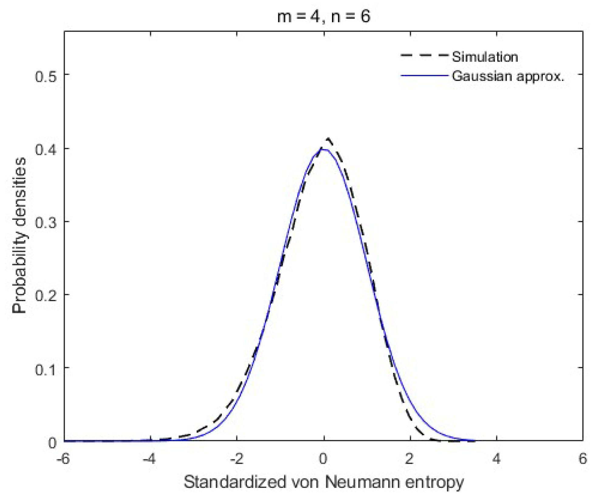
Figure 1. Simulated distribution of Λ when m = 4 , n = 6 .
Preprints 82077 g001
Figure 2. Simulated distribution of Λ when m = 16 , n = 24 .
Preprints 82077 g002
Disclaimer/Publisher’s Note: The statements, opinions and data contained in all publications are solely those of the individual author(s) and contributor(s) and not of MDPI and/or the editor(s). MDPI and/or the editor(s) disclaim responsibility for any injury to people or property resulting from any ideas, methods, instructions or products referred to in the content.
Copyright: This open access article is published under a Creative Commons CC BY 4.0 license, which permit the free download, distribution, and reuse, provided that the author and preprint are cited in any reuse.
Prerpints.org logo

Preprints.org is a free preprint server supported by MDPI in Basel, Switzerland.

Subscribe

© 2024 MDPI (Basel, Switzerland) unless otherwise stated