
Submitted:
10 August 2023
Posted:
11 August 2023
You are already at the latest version
Abstract
We study the robustness of the cμ-rule for the optimal allocation of a resource consisting of one unreliable server to parallel queues with two different classes of customers. The customers in queues can be served with respect to a FCFS retrial discipline, when the customers at the head of queues repeatedly tries to occupy the server in a random time. It is proved that for the scheduling problem in the system without arrivals the cμ-rule minimizes the total average cost. For the system with arrivals it is difficult directly to prove the optimality of the same policy with explicit relations. We derived for an infinite-buffer model a static control policy that also prescribes for the certain values of system parameters the service exclusively for the class-i customers if both of queues are not empty with the aim to minimize the average cost per unit of time. It is also shown that in a finite-buffer case the cμ-rule fails.
Keywords:
Queueing system
; cm-rule
; scheduling problem
; static policy
; average cost
1. Introduction
The modelling and analysis of telecommunications and computer systems is now inconceivable without the various tasks associated with resource allocation and formulated in the framework of the queueing theory. One of such classic problems is to allocate a server to multiple parallel queues with the mostly studied objective to minimize the average cost per unit of time. It was shown that for many systems with such kind of resource allocation problem the allocation policy in form of the -rule is optimal. In literature this rule is also known as Smith’s rule or Weighted Shortest Processing Time. According to this rule the waiting class-i customer from a non-empty queue is allocated to the server if it has a minimal weight of the form , where is a holding cost per unit of time the customer is in the queue or at server and is a overall service rate of the class-i customer. The -rule is a very attractive policy, since it is a static one and requires only the information whether a certain queue is empty or not. Obviously, to apply such a policy the values and must be known, which unfortunately is not always the case, especially for the overall service intensity.
The optimality of the -rule for ordinary multi-class single-server queues in different settings was proved, see e.g. [3,4]. In [16], the authors analyzed the -rule for queueing models with non-linear costs. The optimality of this rule for discrete-time queueing models with a general distributed inter-arrival time and geometrically distributed service time was established in [2]. A concept of a generalized -rule was proposed in [16], where it was shown that this rule is asymptotically optimal for non-decreasing convex delay costs. A classic scheduling problem with a single resource shared by two competing queues was considered in [10] in the context of the stochastic flow model where it was shown that the -rule is optimal. The non-preemptive assignment of a single server to two infinite-capacity retrial queues was analyzed in [18] where -rule was optimal for a scheduling problem in a system without arrivals. The authors in [11] considered the learning-based variants of the -rule where the service rates are unknown.
The constant retrial policy was introduced in [8], where it was assumed that only the customer at the head of the queue can request for service after an exponentially distributed retrial time. The single class queueing systems with constant retrial rate and different options were analysed intensively, e.g. in [6,7,17] and other papers. The uncontrolled analogue of a two-class queueing system has also been investigated by a number of authors. For example, in [1] the authors studied a two-class system with a single exponential service requirements and constant retrial policy. The regenerative approach was used there to derive a set of necessary stability conditions of such a system. The generating function of the stationary distribution of the number of orbiting customers at service completion epochs was obtained in [5].
This paper deals with a controllable unreliable single-server two-class queueing system with constant retrial rates. The optimal allocation problem for this queueing model with retrial and reliability attributes is a new one. The emphases of the paper is on answering the question how robust is the -rule as an optimal allocation policy in the queueing system under study. The queueing system is studied without and with arrivals. In first case explicit relations of the -rule can be derived. In second case, the relations for the optimality of the -rule were obtained for the model with a certain constraint on arrival process.
2. Model description
We analyze the markovian single-server queueing system servicing two classes of customers as illustrated in Figure 1. The customers of each class arrive to the system according to a Poisson stream with a rate . Independently of the state of server the class-i customers join upon arrival the corresponding waiting line or queue with infinite capacity .
The service of customers from the queue occurs according to a FIFO retrial discipline, i.e. the customer waiting at the head of the queue retries to occupy the server in exponentially distributed time with a rate . The server during a service process of the ith-class customer can fail in exponentially distributed time with a rate . In this case the customer leaves the service area and joins again the head of its queue. In failed state the server can be repaired in exponentially distributed time with a rate . All type of time intervals are assumed to be mutually independent. At moments of retrial arrival the idle server may accept the customer of a certain class, who attempts to occupy the server, or can deny the service. The system performance is described by the steady state average cost which is of the form
where is the average number of the ith-class customers present in the system given the allocation policy is f and the holding cost per unit of time the ith-class customer spends in the system. The objective of the present analysis is to provide how robust is a static policy f defined as a -rule for the system under study by minimizing the average cost per unit of time (1).
Denote by the number of ith-class customers in the system at time t and by the state of the server at time t which is defined as follows,
Consider the three-dimensional continuous-time Markov chain
with a state space
and policy-dependent infinitesimal matrix with components for ,
where stands for a vector of dimension 3 with 1 in the ith position, , and 0 elsewhere. Here f is a control policy which prescribes at the moments of retrial arrival the allocation of the ith-class customer to the server. The set of admissible control actions is defined by , where means that upon retrial arrival in state x the ith-class customer must be accepted for service. The sets of admissible control actions in state x is denoted by , where for , , for and for . It is assumed that the stability condition is fulfilled. According to a general result for the system with parallel queues, see e.g. [4], the system is stable if the total load , where the load of the class-i queue. The value can be obtained if we treat the class-i queue as independent single-server queueing system with parameters , , , and . The corresponding continuous-time Markov-chain is then a quasi-birth-and-death (QBD) process with a three-diagonal block infinitesimal matrix
According to a matrix-analytic approach for QBD-processes [12], the queue i is stable if the following inequality holds,
where is a stationary distribution for the infinitesimal transition matrix
which satisfies the system and . The solution of the system is given by
where . By substituting the solution (5) into (4) we get
and the stability condition is then defined as
Below we present the main results of this paper obtained for a system with two classes of customers. However, these results can also be generalized to the case of an arbitrary number of classes.
3. Optimal allocation problem
Consider first a classic scheduling problem for the allocation of customers in the system without arrivals, i.e. when , in which the customers are queued. The waiting customers must be served in such a way that the overall average cost is minimized. It is assumed that the allocation policy and for . Here we have a classical scheduling problem
Proposition 1.
In state the optimal allocation policy can be defined in form of a -rule,
where , , . In case of equality , the control actions 1 and 2 are equivalent.
Proof.
Denote by the total minimal average cost given the initial state is . This function is given by
We need to prove that if as defined in a proposition. First we show that implies . In case and we get from (8), () and () after some simple algebra the relation for ,
In case , if in state the action 2 is chosen instead of the action 1, we get the following inequality,
Now, if is optimal, then the difference of expressions (12) and (13) must be positive, i.e.
what is coincide with a statement.
In case of equality the control actions 1 and 2 are equivalent, i.e. for . We show that the optimal policy and implies that . Note that and for . For the minimum in (8) in case we get then for the control action the relation
in form (12). For the control action the relation
is equal to the right hand side of the inequality (13). The difference of the total average cost given by the relation in (14) for equivalent actions must be equal to zero. Therefore, if , the control action 1 and 2 are equivalent. □
It is assumed now that new customers can arrive to the system, i.e. , . We expect that the same -rule defined in (7) will be optimal for the system with arrivals but from technical reasons it is quite difficult to derive expressions for the mean overall service times of the ith-class customers. Therefore, to analyse the properties of a an optimal control policy we have to introduce a queueing model with a constraint on possible arrivals. This model differs from original one, since we assume that a new arrival can occur only in state , , where the server is empty. The dynamic-programming approach, see e.g. [9], [14,15], is used to establish the properties of the optimal control policy in the following Proposition. Note that the state space of the corresponding Markov decision process (MDP) is infinite and the costs are unbounded. The existence of an average cost optimal stationary policy and convergence of the value-iteration algorithm can be verified in the same way as it was done in [13], where the authors generalized the existence of the optimal policy for the discounted expected total cost minimization to the average cost criterion.
Proposition 2.
In state the optimal allocation policy for the system with a constraint on arrivals can be defined in form
In case of equalities and , the control actions 1 and 2 are equivalent.
Proof.
For the introduced cost structure the average cost stationary optimal policy exists. This policy can be found as a solution of the system of optimality equations for the dynamic-programming relative value function and gain g,
where and is an immediate cost of the corresponding MDP. In states with the only one nonempty queue the optimal policy consists in service of the corresponding customer, the relative value functions are of the form,
where . The value , then . The equations for states where the server is busy or failed are
The solution for the system of optimality equations can be calculated recursively using equivalent discrete-time model on a finite horizon obtained by an uniformization procedure. The corresponding recursive relations have almost the same structure. Namely, the equations (22)–(24) can be rewritten in such a way that on the left-hand side the function is replaced by the -stage cost function and on the right-hand side we put and function is replaced by the n-stage cost function . It is assumed that the initial condition is , . Let the inequalities in the first raw of (15) hold. Consider the term for action selection in obtained recursive relations. In case
for any , the optimal control action is for an arbitrary n. The statement is proved by induction on n. If , the inequality (25) obviously holds. Assume the validity of this inequality for some n. Then it must be proved that (25) holds for . Expressions for , and can be obtained from (22)–(24). The first terms by in inequality (25) are multiplied by the factor defined as
In case , , we obtain from (25) the following inequality,
where we multiply the first term in the left- and right-hand side by the factor . The inequality (26) which is valid due to the following reasons. For the terms with the factor by adding to the left-hand side the item and to the right-hand side the item we get,
The inequality (27) holds due to the induction assumption (25) in state . In the same way prove the inequality for the terms with the factor . In this case we add to the left-hand side and right-hand side of the corresponding inequality respectively the elements and to the right-hand side . The the induction assumption (25) in state can be applied. The inequality obtained for the terms with a factor by subtracting and respectively from the left-hand side and right-hand side holds as well due to the induction assumption in state . The inequalities for the terms with factors and satisfy directly the induction assumption (25). The rest of terms builds the inequality of the form
After some simple algebra we get from (28) the inequality
or by means of the variable it is of the form
The inequality (29) holds due to the assumptions for the control action 1, i.e. and and the inequality
obtained directly from the stability condition (6). In fact, the expressions in brackets of the inequality (29) can be rewritten respectively as
The second expression in (30) is obviously non-negative, due to conditions and . If
then (29) is true. If
then
that confirms the validity of the inequality (29).
The inequality (25) for can be proved using the same technique as before. Indeed, the inequality (26) is converted to
By further comparing the terms of the corresponding inequality for the parameters of the system, we obtain inequality (29) using the proof by induction as for the case . And finally we note that the inequalities in (15) automatically lead to the -rule defined in (7), but this doesn’t always hold true vice - versa. □
Conjecture 1.
We expect that the policy defined by (15) is also optimal for the system where a constraint on arrival is omitted. This can be explained by the fact that the proportion of the class-i customers arrived to the system during the time when the server was idle will also be maintained when customers arrive in states where the server is busy or in a failed state. Therefore, the incentive to service the customer of a certain class remains the same and hence the policy (15) seems to be valid for the original queueing system with arrivals.
Example 1.
Consider the system with fixed parameters and six cases of varied parameters given in Table 1. The last two columns of the table represents the values of the average cost g evaluated using a simulation technique for the policy with and , .
The inequalities from (15) are:
In Case 3 we get equivalent policies, the simulation results for the average cost are very similar. In Cases 5 and 6 the relations are converse, but the optimal policy, as expected, still follows the rule .
For the system with finite buffer capacities the optimal allocation policy can have in general another structure then the -rule due to the influence of boundary states. In the next example we illustrate such a result.
Example 2.
Consider the system with parameters of Case 4 from Example 1 and finite buffer capacity for both of queues . The state-dependent optimal control actions evaluated by a dynamic-programming approach are summarized as a matrix represented in Table 2. The columns describe the number of customers in a queue 1 and the rows – in a queue 2. It can be seen that the optimal policy is not a static any more.
The optimal average cost here is . The average cost for the policy , , is equal to and for the policy , , the average cost takes lower value . This results for the optimal policy differ from those obtained for higher buffer capacities. As and increase, the boundary between areas 1 and 2 in a control matrix shifts right. In infinite buffer case, the optimal policy is defined exclusively by actions , , with the average cost , while the alternative policy , , leads now to the higher average cost .
4. Conclusion
In this paper we have analyzed the optimal routing problem for the unreliable single-server two-class queueing system with constant retrial rates. We derived conditions for the optimality of a static policy to serve the customers from a certain queue. The system without new arrivals can be treated as a ordinary multi-class system with a generally distributed service time. For the system with new arrivals a -rule cannot be used directly. We have provided a dynamic programming approach to find explicit conditions when static control policies are guaranteed to be optimal.
References
- Avrachenkov, K.; Morozov, E.; Nekrasova, R.; Steyaert, B. Stability analysis and simulation of n-class retrial system with constant retrial rates and poisson inputs. Asia-Pacific J. Oper. Res. 2014, 31. [Google Scholar] [CrossRef]
- Baras, J.S.; Dorsey, A.J.; Makowski, A.M. Two competing queues with linear costs and geometric service requirements: The μc-rule is often optimal. Advances in Applied Probability 1985, 17, 186–209. [Google Scholar] [CrossRef]
- Buyukkoc, C.; Varaiya, P.; Walrand, J. The cμ rule revisited. Advances in Applied Probability 1985, 17(1), 237–238. [Google Scholar] [CrossRef]
- Cox, D.R.; Smith, W.L. Queues; Methuen: London, 1961. [Google Scholar]
- Dimitriou, I. A two-class queueing system with constant retrial policy and general class dependent service times. Eur. J. Oper. Res. 2018, 270, 1063–1073. [Google Scholar] [CrossRef]
- Economou, A.; Kanta, S. Equilibrium customer strategies and social-profit maximization in the single-server constant retrial queue. Nav. Res. Logist. (NRL) 2011, 58, 107–122. [Google Scholar] [CrossRef]
- Efrosinin, D.; Winkler, A. Queueing system with a constant retrial rate, non-reliable server and threshold-based recovery. Eur. J. Oper. Res. 2011, 210, 594–605. [Google Scholar] [CrossRef]
- Fayolle, G. A simple telephone exchange with delayed feedbacks. In Proceedings of the international seminar on Teletraffic analysis and computer performance evaluation, Amsterdam, The Netherlands; 1986; pp. 245–253. [Google Scholar]
- Howard, R.A. Dynamic programming and Markov processes (technology press research monographs) (), 1st ed.; MIT Press: Cambridge, 1960. [Google Scholar]
- Kebarighotbi, A.; Cassandras, C.G. Revisiting the optimality of the cμ-rule with Stochastic Flow Models. In Proceedings of the 48h IEEE Conference on Decision and Control (CDC) held jointly with 2009 28th Chinese Control Conference; 2009. [Google Scholar]
- Krishnasamy, S.; Arapostathis, A.; Johari, R.; Shakkottai, S. On Learning the cμ Rule in Single and Parallel Server Networks. 2018. [Google Scholar] [CrossRef]
- Heyde, C.C.; Neuts, M.F. Matrix-Geometric Solutions in Stochastic Models. An Algorithmic Approach. J. Am. Stat. Assoc. 1982, 77, 690. [Google Scholar] [CrossRef]
- Özkan, E.; Kharoufeh, J. Optimal control of a two-server queueing system with failures. Probability in the Engineering and Informational Sciences 2014, 28, 489–527. [Google Scholar] [CrossRef]
- Puterman, M.L. Markov decision processes: discrete stochastic dynamic programming; Wiley-Interscience: New York, 1994. [Google Scholar]
- Sennott, L.T. Stochastic dynamic programming and the control of queueing systems. Wiley series in probability and statistics: applied probability and statistics; Wiley: Wiley.
- Van Mieghem, J.A. Dynamic scheduling with convex delay costs: The generalized cμ-rule. The Annals of Applied Probability 1995, 5, 809–833. [Google Scholar] [CrossRef]
- Wang, J.; Zhang, X.; Huang, P. Strategic behavior and social optimization in a constant retrial queue with the N -policy. Eur. J. Oper. Res. 2016, 256, 841–849. [Google Scholar] [CrossRef]
- Winkler, A. Dynamic scheduling of a single-server two-class queue with constant retrial policy. Ann. Oper. Res. 2011, 202, 197–210. [Google Scholar] [CrossRef]
Figure 1.
Schema of the single server two-class controllable queueing system
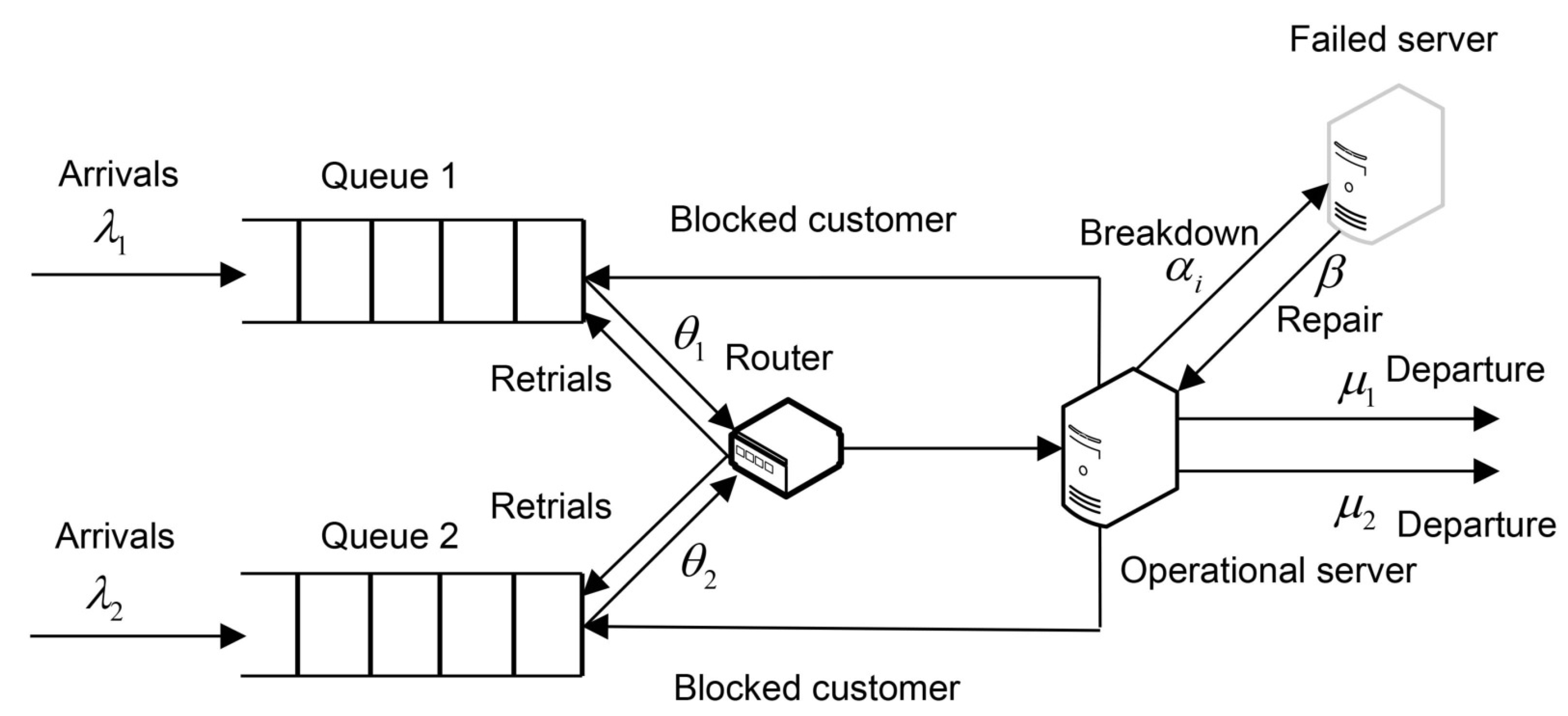

Table 1.
Simulation results
| 0.30 | 5 | 3 | 0.55 | 0.5 | 0.10 | 1.00 | 25.657 | 29.403 |
| 0.26 | 5 | 3 | 0.70 | 0.40 | 0.10 | 2.00 | 36.909 | 34.238 |
| 0.26 | 5 | 3 | 0.70 | 0.43 | 0.12 | 1.64 | 18.223 | 18.291 |
| 0.30 | 3 | 5 | 0.51 | 0.5 | 0.10 | 1.00 | 25.430 | 22.955 |
| 0.30 | 3 | 5 | 0.51 | 0.5 | 0.10 | 0.90 | 23.421 | 24.709 |
| 0.30 | 5 | 3 | 0.55 | 0.5 | 0.10 | 1.20 | 33.348 | 31.610 |
Table 2.
Matrix of optimal control actions
| \ | 0 | 1 | 2 | 3 | 4 | 5 | 6 | 7 | 8 | 9 | 10 | ⋯ |
|---|---|---|---|---|---|---|---|---|---|---|---|---|
| 0 | 0 | 2 | 2 | 2 | 2 | 2 | 2 | 2 | 2 | 2 | 2 | ... |
| 1 | 1 | 2 | 2 | 2 | 2 | 2 | 2 | 2 | 2 | 2 | 2 | ... |
| 2 | 1 | 2 | 2 | 2 | 2 | 2 | 2 | 2 | 2 | 2 | 2 | ... |
| 3 | 1 | 2 | 2 | 2 | 2 | 2 | 2 | 2 | 2 | 2 | 1 | ... |
| 4 | 1 | 2 | 2 | 2 | 2 | 2 | 2 | 2 | 2 | 1 | 1 | ... |
| 5 | 1 | 2 | 2 | 2 | 2 | 2 | 2 | 1 | 1 | 1 | 1 | ... |
| 6 | 1 | 2 | 2 | 2 | 2 | 1 | 1 | 1 | 1 | 1 | 1 | ... |
| 7 | 1 | 2 | 2 | 2 | 1 | 1 | 1 | 1 | 1 | 1 | 1 | ... |
| 8 | 1 | 2 | 1 | 1 | 1 | 1 | 1 | 1 | 1 | 1 | 1 | ... |
| 9 | 1 | 1 | 1 | 1 | 1 | 1 | 1 | 1 | 1 | 1 | 1 | ... |
| ⋮ | ⋮ | ⋮ | ⋮ | ⋮ | ⋮ | ⋮ | ⋮ | ⋮ | ⋮ | ⋮ | ⋮ | ⋱ |
Disclaimer/Publisher’s Note: The statements, opinions and data contained in all publications are solely those of the individual author(s) and contributor(s) and not of MDPI and/or the editor(s). MDPI and/or the editor(s) disclaim responsibility for any injury to people or property resulting from any ideas, methods, instructions or products referred to in the content. |
© 2023 by the authors. Licensee MDPI, Basel, Switzerland. This article is an open access article distributed under the terms and conditions of the Creative Commons Attribution (CC BY) license (http://creativecommons.org/licenses/by/4.0/).
Copyright: This open access article is published under a Creative Commons CC BY 4.0 license, which permit the free download, distribution, and reuse, provided that the author and preprint are cited in any reuse.


