Preprint
Article

Does Living Near Public Transport Equate to Food (In)security in the United States? – Evidence from the 2020 National Health Interview Survey (NHIS)

Altmetrics

Downloads

123

Views

110

Comments

0

A peer-reviewed article of this preprint also exists.

Submitted:

13 August 2023

Posted:

14 August 2023

You are already at the latest version

Alerts
Abstract
Food security is intrinsically related to health and well-being. This paper investigates the status-quo of food insecurity among the population residing close to transit in various parts of the United States of America (USA). The data from the 2020 National Health Interview Survey (NHIS) collected by the National Center for Health Statistics (NCHS) of the USA are analyzed in this research. Logistic regression is carried out by treating food insecurity as the dependent variable and socioeconomic variables such as age, income, education and dependency on the Supplemental Nutrition Assistance Program (SNAP) as independent variables. Food insecurity is assessed with aggregated information on four aspects of inputs from those respondents who live near a transit: 1) worry food would run out, 2) food didn't last, 3) couldn't afford to eat balanced meals, and 4) cut the size of meals or skip meals. Findings suggest that respondents who live close to transit in the USA and are from large central metro counties of the Northeast, Southern and Western states showed an increase in food insecurity if they were below 65 years of age, had income below country’s median income or their educational attainment was below bachelor’s degree. There was a significant association found between food insecurity of respondents living close to transit and subscribed to using food stamps or SNAP. Policies that could alleviate food insecurity by reducing cost of living near transit are recommended.
Keywords: 
Subject: Social Sciences  -   Transportation

1. Introduction

“Food security” is the basic need of humans critical to creating a healthy and sustainable society. Food security meeting the nutritional needs of urban and rural populations has widespread socioeconomic impacts through the network of food aggregators in a supply-chain context. In this process, transportation plays a vital role by facilitating and upholding food security through the much-needed circulation of food for the masses. However, very little is known about how people relocate close to a transportation system to ensure their food security is met or unmet as they reside close to the transportation facilities. In addition, the success of food security must be gauged by its ability to feed the last consumer in the food supply chain, especially those who belong to low-income communities residing near public transport. This again needs some current understanding of the existing food insecurity among the residents near transit, requiring further policy discussion and research, which this paper investigates. Therefore, the objective of this paper is to develop our understanding of how food security (if at all) is prevalent among people residing near transit, or, in other words, investigating if living near public transport equate to food (in)security or vice-versa. We use the data from the United States of America (USA), as an example, to answer this research question.
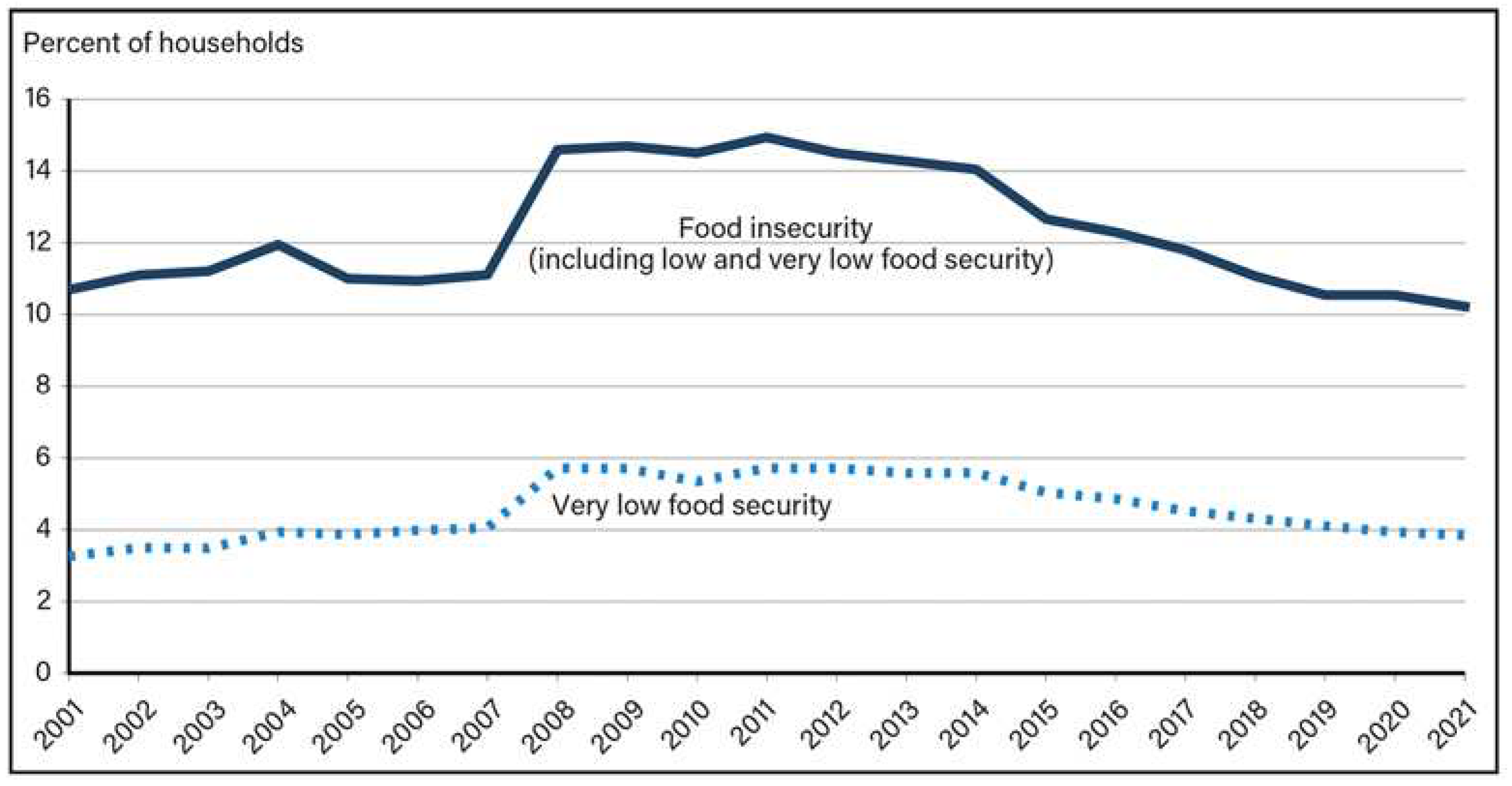
Food insecurity has been identified as a public health and environmental issue affecting many people in the United States ([1,2]). Lack of access to adequate food in the US arise because of poor financial and resource availability [1] – since food insecurity is mainly prevalent in families with low-income, are disabled or belong to minority races [3]. In 2021, there were 13.5 million households in the US who were food insecure, determined by many factors, including household circumstances, the economy, and Federal, State, and local policies [4]. The chart in Fig. 1 shows how food insecurity has been prevalent over the years in US households from 2001 to 2021.
Figure 1. Trends in food insecurity in US households, 2001-21 (Source: USDA, Economic Research Service using data from US Department of Commerce, Bureau of the Census, Current Population Survey Food Security Supplements [4]).
Preprints 82297 g001
The United Nations has defined food security as when “all people, at all times, have physical, social, and economic access to sufficient, safe, and nutritious food that meets their food preferences and dietary needs for an active and healthy life” [5]. The World Food Programme (WFP) of the United Nations, focusing on food security and hunger, points out that in 2022, 879 million people did not have sufficient food consumption across 92 countries worldwide. About half of these are from Asia and the Pacific, with India having the largest population, predicted to have about 244 million people with insufficient food consumption [6].
Various studies show that the integration of agriculture and political will combined with the logistics of food delivery can ensure food security [7]. However, the process cannot be entirely successful unless an effective public policy with strong implementation measures exists on food security. In the USA, Food Stamp Program, now known as the Supplemental Nutrition Assistance Program (SNAP), provides nutritional benefits to supplement the food budget of needy families and enables them to purchase healthy food [8]. The SNAP aims to help those that meet the requirements with income below certain gross and net income limits for given household size. It is expected that the households would spend about 30 percent of their resources on food. Thus, for a household size of 1, the maximum monthly benefits (known as ‘allotment’) for 2021-2022 is fixed at $250. The allotment is calculated by multiplying a household’s net monthly income by 0.3 and subtracting the result from the maximum monthly allotment for your household size. Thus, the country's federal government ensures food security for the household.
Transportation plays a critical role in food security and ensuring that every individual has access to various food production sources and markets. As per the Centers for Disease Control and Prevention (CDC) – “A poor transportation system cuts off access to many food outlets—especially for those who do not own a car or have no access to reliable and affordable public transportation.” A strong nexus among the three, namely the farmers (as food producers), retailers, and consumers facilitated by transport, ensure an appropriate level of food security is guaranteed for all. Often it is a challenge for some to travel to stores to purchase food. Transit or other cheap nonmotorized transport is a natural choice for low-income households to access food stores. Over the last few decades, investments in public transport in the US have been steadily increasing to stimulate ridership and provide an alternate mode of transportation (addressing equity issues) to low-income communities [9]. Successful investment planning for transit has also led to decentralizing poverty in the suburbs [10]. However, transit improvements and development often lead to gentrification and socioeconomic changes over time in low-income neighborhoods that already reside close to transit. This can severely paralyze policies meant to uplift low-income households that earn their daily livelihood by continued use of public transport. A recent study by Liang et al. (2022) showed that a new rail line increased the number of advanced degree holders in the proximity of the rail line in the City of Hong Kong [11]. This indicates that rail transit investment induces high-educated people to move into transit-rich low-income areas, thereby compelling low-income households to move out and away from being able to access transit to fulfill daily commuting needs. In another study, for the city of Rosengård in Malmö in Sweden, gentrification and displacement of low-income neighborhoods were observed with the transit-orient development programs [12]. Similar debates in the media have been on ensuring affordable housing for low-income groups in cities like Delhi [13].
In developed nations like the USA, dense urban areas where food consumption is the highest because of the high population, the cost of living (housing) and commuting for low-income commuters to access food often pose a significant challenge. To minimize housing costs and prevent the movement of low-income households from transit-rich locations, various cities in developed nations like the USA have taken steps to provide affordable housing for low-income families. For example, the densely populated City of Long Beach in California has seen a surge in several affordable housing projects close to the A Line transit of the Los Angeles Metro area in the past five years [14] . The A Line transit serves a large community of low-income households.
The map in Fig. 2a shows the percentage of SNAP participants in the year 2020 across the four analyzed regions of the aggregated States (Data source: USDA, 2023 [28]). Clearly, the subscription of SNAP has been the highest in the Southern states compared to the others. Subsequently, using the data from the American Community Survey (ACS) [15], the latest commuting patterns across the four regions were compared to the percentage of SNAP subscription. The percentage distribution of workers commuting by transit is shown in Fig. 2b, which points out the least transit usage by the Southern states. Therefore, this preliminary analysis showed that, although the transit use is minimum in the Southern States, the reliance on SNAP among the residents living close to transit is high in these states. This motivates further research to be conducted surrounding a specific transit line for any required city or town to understand if commuters residing near the transit use transit, have a significant subscription to SNAP, which could reduce food insecurity addressed in this paper.
Figure 2. Percentage distribution of SNAP participants and transit commuters across regions of the USA.
Preprints 82297 g002
Studies have shown that along with welfare benefits and socioeconomic factors, food security depends on proximity to retail grocery stores and food prices ([16,17]), and public transport is a natural mode for low-income households to access such retail stores. In another study, Baek (2014) concluded that an extra bus-equivalent vehicle serving 10,000 people decreases the probability of food insecurity by 1.6 percent [18].
Personal vehicles serve as the first mode of choice to access food stores in urban areas that are deprived of an efficient and reliable public transportation system [19]. Studies to develop the relationship between the spatial availability of food and the influence of travel mode and travel time necessary to purchase food have also been well-documented [20]. Prior studies have shown that for the City of Baltimore in the US, residents with lack of food stores had a significantly high travel time compared to those living in communities who were close to a supermarket [21]. Findings from other cities of the US, such as San Diego, showed that minimum travel time by car to any store was 4.22 minutes, while it was 15.88 minutes with transit [20]. All of these examples show availability of transit does not guarantee efficiency in access to food in a developed nation. Thus, this topic of research is much of interest for investigating if transit helps attenuate food insecurity in the USA.
However, to our knowledge, no research has been conducted to evaluate the association between living near transit and food security among Americans. This paper investigates if those living near transit in the USA are also the ones who are facing food insecurity- and if yes, it would serve as a worthwhile motivation to identify policies that would minimize food insecurity for a healthy society thriving on transit for daily needs. To the best of our knowledge, this is the first study conducted on this issue of food security among the population residing near transit, which can be replicated for other regions of the world with similar demographics to the USA.
In essence, this paper evaluates the impacts of various factors on food insecurity among the American population residing near public transport. Factors that are key socioeconomic variables such as age, income, education level, and dependency on food stamps in the last twelve months are studied for food insecurity measured across four combined inputs gathered on the following information from the respondents living near transit if they, in the past, had to - i) worry food would run out, ii) food didn't last, iii) couldn't afford to eat balanced meals, and iv) cut the size of meals or skip meals. The source of this information is further discussed in detail in the next section. In the next section, we describe the methodology used in this paper to deduce the above findings on food security for those residing near transit.

2. Materials and Methods

2.1. Regression Analysis

In this research, food insecurity is the modeled output variable. Food insecurity, as the dependent variable, assumes a binary value with a dichotomous output. When its value is equal to 1, it indicates that food insecurity is 1; when it is equal to 0, it indicates food security. With this assumption, a logistic regression fits the best as the method to understand how various socioeconomic explanatory variables impact food insecurity. Research manuscripts reporting large datasets that are deposited in a publicly available database should specify where the data have been deposited and provide the relevant accession numbers. If the accession numbers have not yet been obtained at the time of submission, please state that they will be provided during review. They must be provided prior to publication.
A brief theoretical background of the logistic regression applicable in statistical modeling for dichotomous outputs with X being a vector of explanatory variables is provided below (source: [22]):
log ( π 1 π ) = β X i
where,
π is the probability of an event, and β are the estimated coefficients. The coefficient estimation is determined using the principle of maximum likelihood technique, with n observations:
L ( β | X i ) = i = 1 n π Y i ( 1 π ) 1 Y i
Using natural logarithm on Eq. (2) gives a sum for the likelihood function as,
log { L ( β | X i ) } = i = 1 n [ Y i log π + ( 1 Y i ) log ( 1 π ) ]
Maximizing the log-likelihood equation in Eq. (3) by finding the first derivative and equating it to zero, will give the estimation of the coefficients, β. Various statistical software packages can be used to carry-out logistic regression for the theoretical information presented above. However, it must be noted that it is necessary to identify the socioeconomic variables as categorical or continuous variables before performing the regression.
Furthermore, we use the odds ratio to quantify the association between food insecurity and each of the individual variables. The odds ratio in the context of this research is defined as the ratio of the odds of an independent variable that causes food insecurity to the odds of the same variable not impacting food insecurity. Mathematically, the odds ratio is calculated based on information presented in the contingency Table 1 and the formula is:
(Odds ratio) = (X22/ X21)/(X12/ X11)
where,
X11 = number of times in the data the value of the independent variable is 0, with food security
X12 = number of times in the data the value of the independent variable is 0, with food insecurity
X21 = number of times in the data the value of the independent variable is 1, with food security
X22 = number of times in the data the value of the independent variable is 1, with food insecurity
The significance of the odds ratio is that if it is greater than 1, it ‘indicates a positive association between the independent variable and food insecurity. An odds ratio less than 1 indicates a negative association, while a ratio equal to 1 indicates no association between the independent variable and food insecurity.
Table 1. Contingency table.
Food insecurity
0 1
Independent Variable 0 X11 X12
1 X21 X22

3. Application Example

3.1. Study Region and Data Collection

Data from the 2020 National Health Interview Survey (NHIS) collected by the National Center for Health Statistics (NCHS) of the USA are analyzed in this research. Although the NHIS data primarily focuses on health-related information of the noninstitutionalized population of the US, the survey, for the first time in the year 2020, includes information on those populations that reside near transit while inquiring about their food security status.
Based on the survey documentation, it has been pointed out that, in 2020, due to the COVID-19 pandemic, data collection procedures were disrupted. From April to June, all interviews were conducted by telephone only. From July to December, interviews were attempted by telephone first, with follow-ups to complete interviews by personal visit. In this way, 31,568 sample adult interviews were carried out [23]. The information from these many sample interviews is publicly available for researchers. Our primary focus was to extract only the relevant information on food (in)security, residing status of respondents if located near transit and their socioeconomic characteristics. There were 15,786 respondents who lived within walking distance (or close to a transit stop) at the time of the interview.
The 2020 National Health Interview Survey (NHIS) data on food insecurity and associated explanatory variables were at the spatial scale of counties spanning four regions of aggregated states, namely the Northeast, Midwest, South, and Western. Further, the counties within these aggregated states were classified based on the 2013 NCHS Urban–Rural Classification Scheme [24] . This classification scheme is based on the county population. It has six divisions: four metropolitans (large central metro, large fringe metro, medium metro, and small metro) and two nonmetropolitan (micropolitan and noncore).
A county that is a large central metro is defined as in metropolitan statistical area (MSA) of 1 million or more population that with the entire population of the largest principal city of the MSA. A large fringe metro has a population size between 1 million or more, which does not qualify as large central metro county. A medium metro county in MSAs has a population of 250,000 to 999,999, whereas a small metro county in MSAs has a population of less than 250,000. The nonmetropolitan categories of micropolitan and noncore are the respective counties in micropolitan statistical areas and the nonmetropolitan counties that did not qualify as micropolitan.
However, the survey combines the data from medium and small metro county respondents into one, and the same was done for the micropolitan and noncore nonmetropolitan counties. Thus, instead of six classification counties of the 2013 NCHS Urban-Rural Classification Scheme, the survey data has information on four levels of county classification: large central metro, large fringe metro, medium and small metro, and nonmetropolitan.
The association between the likelihood of facing food insecurity by the survey respondents residing close to transit and the socioeconomic variables of age, income, education level, and dependency on food stamps were estimated for significance using logistic regression. Note that the socioeconomic variables, as well as the food insecurity, were treated as dichotomous variables. Table 2 shows each variable definition used in the logistic regression. It is noted that the age of 38.6 years was identified as a classification level based on the 2020 median age of the US population. The purpose of keeping the median age as a classification level was to understand if there was any significance in food insecurity below this age among the respondents.
Further, the income levels were classified based on the poverty and median household incomes of $21,960 and $67,521, respectively. With an income that is below the poverty benchmark, it would be expected that food insecurity might be a concern among those living near transit. Like median age, median income was a natural choice as a classification level in understanding food insecurity.
Education as the explanatory variable was classified based on the respondents’ qualifications in holding a degree, i.e., if the respondent had a degree, was it an associate degree, a bachelor’s, or a higher educational degree. The purpose was to understand if food security was at all impacted among the respondents with their level of educational attainment.
The last variable tested for impact on food insecurity is the respondents’ utilizing food stamps in the previous twelve months. Availing food stamps or the SNAP by respondents would not mean food insecurity occurs. Since, SNAP is intended to eliminate food insecurity that stems from worrying if the food would not last, run out, or the respondent has to cut the size of meals or skip meals.
Table 2. Variables definition.
Variable Notation Coding
Male Male 1 = Male, 0 otherwise
Age ≤ 38.6 (USA 2020 Median age: 38.6α) Age_386 1 if Age ≤ 38.6, 0 otherwise
Age in-between 38.6 and 50 Age_38650 1 if 38.6 < Age ≤ 50, 0 otherwise
Age in-between 50-65 Age_5065 1 if 50 < Age ≤ 65, 0 otherwise
Age > 65 Age_65 1 if Age > 65, 0 otherwise
Income ≤ $21,960 (below poverty with a mean family size of 3β) Inc_p 1 if Income ≤ $21,960, 0 otherwise
Income $21,960 to $67,521 (Median household income in the USA was $67,521 in 2020γ) Inc_pm 1 if $21,960 < Income ≤ $67,521, 0 otherwise
Income > $67,521 Inc_m 1 if Income > $67,521, 0 otherwise
Education level with no degree Edu_nd 1 if Education with no degree, 0 otherwise
Education level with associate degree and aboveθ but below bachelor level Edu_ad 1 if Education with a degree below undergraduate, 0 otherwise
Education level with bachelors and above degree Edu_bd 1 if Education with undergraduate and above degree, 0 otherwise
Received food stamp in the last 12 months Food_S 1 if received food stamp in last 12 months, 0 otherwise
αSource: Statistica.com, 2021 [25]; βSource: Statistica.com 2021 [27]; γUS Department of Health and Human Services, 2021 [26]; θAssociate degree in occupational, technical, vocational program, academic program etc.
A total of sixteen spatially distinct scenarios covering almost the entire US were analyzed. These scenarios were from four of the 2013 NCHS Urban–Rural Classification Scheme counties times the four aggregated states, Northeast, Midwest, South, and West.
Table 3 shows the descriptive statistics for the explanatory variables. The table was prepared for those respondents living close to transit.
A very high percentage of almost 94% respondents living near transit and in the large central metro counties of the Northeast states indicated food insecurity. The percentage of respondents living near transit and in the nonmetropolitan counties of the South states had the lowest (8%) food insecurity. Overall, for the respondents living near a transit and in the nonmetropolitan counties of the Midwest and South states, the percentages of explanatory variables were found to be lower than in the other two regions of the aggregated states. The percentage distributions of all the explanatory variables were the largest for the large central metro counties across all the four regions of the aggregated states.
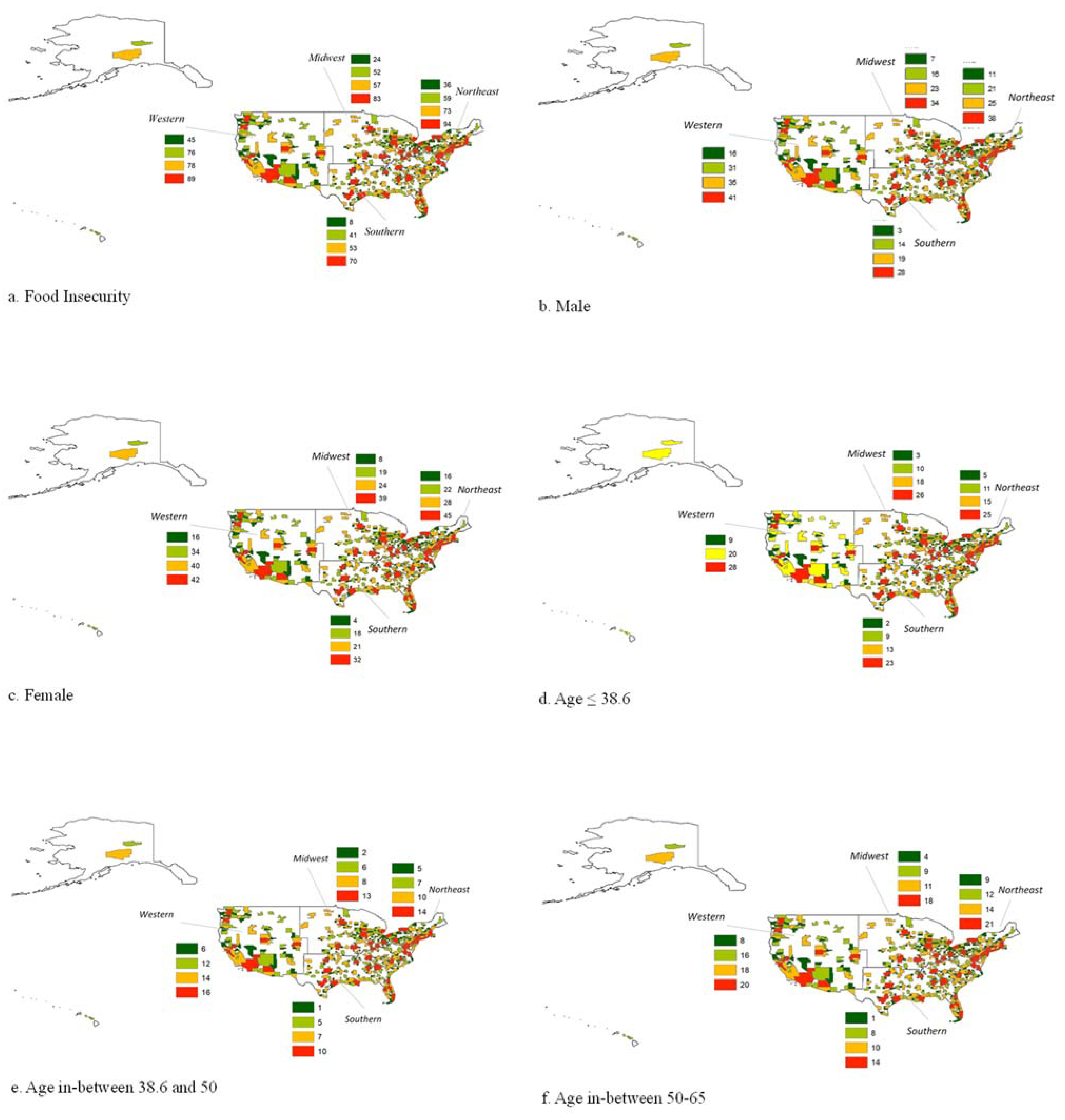
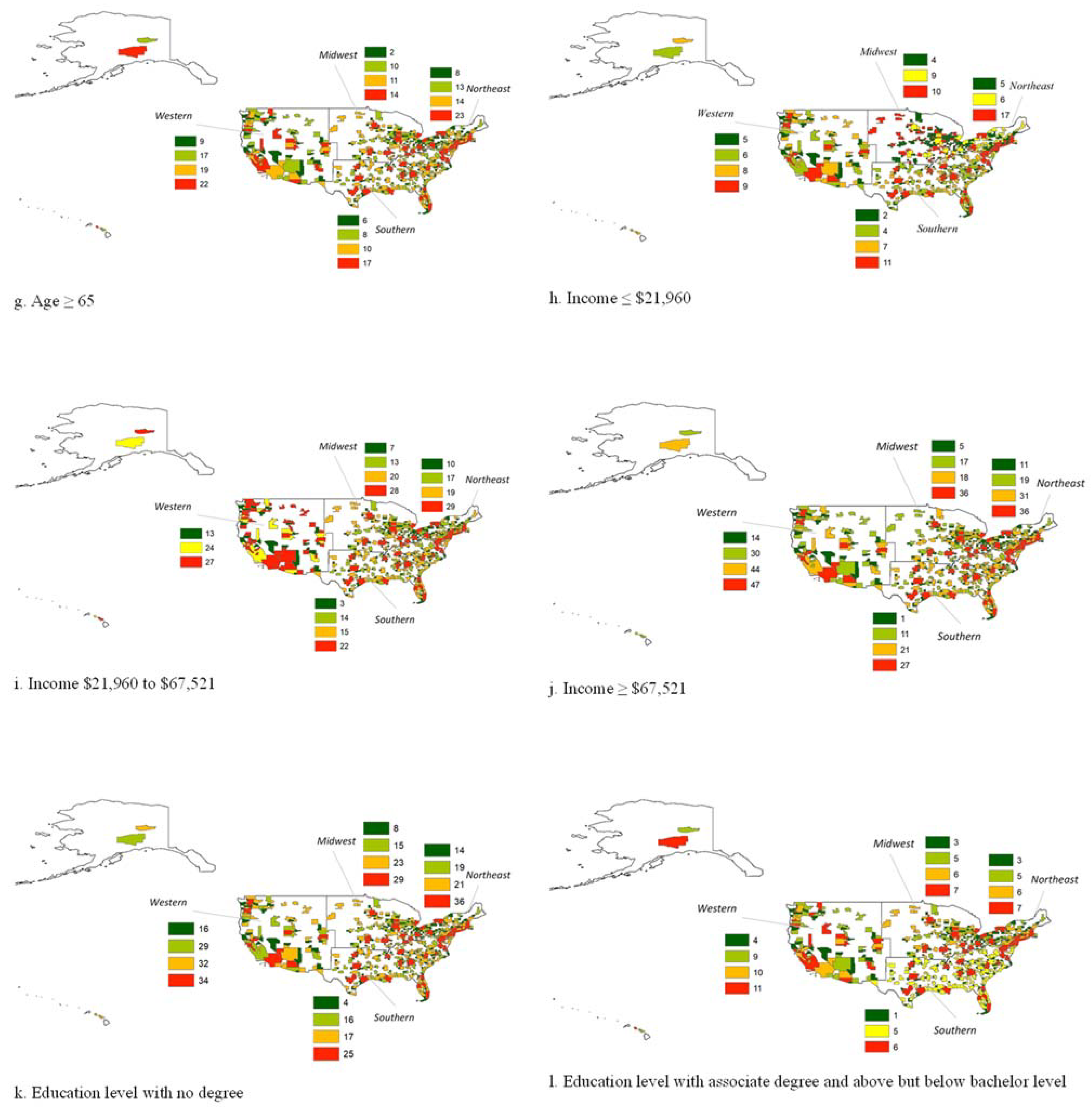
The maps in Figs. 3-5 show the spatial variations in the percentages of the food insecurity and the thirteen explanatory variables. The map of food insecurity, the gender variables (males and females, age of respondents between 38.5 to 50 years and 50 years to 65 years, income greater than $67.5k and education level bachelors and above appear to have a similar color shade – although differing in their respective percentages.
Table 3. Descriptive statistics of the dependent and explanatory variables (shown as percentages)
Variable Aggregated States
Northeast States Midwest States Southern States Western States
Large central metro Large fringe metro Medium and small metro Nonmetropolitan Large central metro Large fringe metro Medium and small metro Nonmetropolitan Large central metro Large fringe metro Medium and small metro Nonmetropolitan Large central metro Large fringe metro Medium and small metro Nonmetropolitan
Food Insecurity
(consists of aggregated affirmative responses to - ‘worry food would run out’, ‘food didn't last’, ‘couldn't afford to eat balanced meals’, and ‘cut the size of meals or skip meals’)
94 73 59 36 83 52 57 24 70 53 41 8 89 78 76 45
Male 38 25 21 11 34 16 23 7 28 19 14 3 41 35 31 16
Female 45 28 22 16 39 19 24 8 32 21 18 4 42 40 34 16
Age ≤ 38.6 (USA 2020 Median age: 38.6) 25 15 11 5 26 10 18 3 23 13 9 2 28 20 20 9
Age in-between 38.6 and 50 14 10 7 5 13 6 8 2 10 7 5 1 16 14 12 6
Age in-between 50-65 21 14 12 9 18 9 11 4 14 10 8 1 20 18 16 8
Age ≥ 65 23 14 13 8 17 8 10 6 14 11 10 2 19 22 17 9
Income ≤ $21,960 (below poverty with a mean family size of 3) 17 5 6 6 9 4 10 4 11 4 7 2 9 6 8 5
Income $21,960 to $67,521 (Median household income in the USA was $67,521 in 2020) 29 17 19 10 28 13 20 7 22 15 14 3 27 24 27 13
Income ≥ $67,521 36 31 19 11 36 18 17 5 27 21 11 1 47 44 30 14
Education level with no degree 36 21 19 14 29 15 23 8 25 17 16 4 34 29 32 16
Education level with associate degree and above but below bachelor level 7 6 5 3 7 5 6 3 6 5 5 1 10 11 9 4
Education level with bachelors and above degree 39 25 19 10 37 15 17 5 29 19 11 2 40 34 23 11
Received food stamp in the last 12 months (2019) 15 9 11 19 10 9 14 14 12 9 15 24 8 7 12 17
Figure 3. Spatial distribution of percentages of explanatory variables – a. Food insecurity, b. Male, c. Female, d. Age ≤ 38.6, e. Age in-between 38.6 and 50, and f. Age in-between 50-65.
Preprints 82297 g003
Figure 4. Spatial distribution of percentages of explanatory variables – g. Age ≥ 65, h. Income ≤ $21,960, i. Income $21,960 to $67,521, j. Income ≥ $67,521, k. Education level with no degree, and l. Education level with associate degree and above but below bachelor level.
Preprints 82297 g004
Figure 5. Spatial distribution of percentages of explanatory variables – m. Education level with bachelors and above degree and n. Received food stamp in the last 12 months.
Preprints 82297 g005

Results and Discussion

The results have been prepared for those population that reside near to transit stop. Hence, the discussion here (for the variables and food (in)security) pertain only to those population.
With the data for the study region at the spatial scale of counties spanning four regions of aggregated states, namely the Northeast, Midwest, Southern, and Western of the USA, Logistic regression results were obtained using the SPSS Statistics 22. The significance level was set at 5%.
Cox and Snell R2 for all the sixteen analysis regions are found to be within 0.2-0.4. It was also observed from the collinearity matrix for each scenario that majority of the explanatory variables showed no strong correlation. In addition, the classification table (confusion matrix) showed that the predicted percentage for food insecurity was above 90% for each of the sixteen scenarios. Based on the output from the software, coefficient estimates of the explanatory variables (along with the standard error for each estimate) have been compiled, as shown in Table 4: at 1% and 5% significance level. It is noted in Table 4 that the values that are missing were found to be not significant at 5% level considered for all outputs of the estimates, and hence, these outputs have not been supplied in the Table 4 for any further discussion or focus. A majority of the coefficient estimates under the columns of nonmetropolitan counties of the Northeast, South, and West have been greyed out, indicating the estimates were not significant at 1% level or at 5% significance level.
The following variables were considered as the base for the categorical variables in the regression for the respondents if they were above the age of 65 (Age_65), had income higher than the country’s median income of $67,521 (Inc_m), and education level with a bachelor’s or a higher degree (Edu_bd). This consideration for respondents was likely not to affect food insecurity which was modeled as the dependent variable – since we expect that food insecurity would be absent among those above 65 because of several welfare schemes meant for the older people such as social security. Further, a respondent possessing a bachelor’s or a higher education qualification with a degree would not have to worry about food security. And finally, income above the median income (much above the poverty threshold) would very unlikely compel a respondent to worry about food being running out or were forced to cut a meal.
The coefficient estimates provided in Table 4 suggest that, at 5% significance level, a decreasing effect of food insecurity exists among males living close to transit for the medium and small metro counties of the Midwest states of the USA. However, similar observations are made for the West states for the large fringe metro counties. Respondents who live close to transit in the USA and in the large central metro counties of the Northeast, Southern and Western states showed an increase in food insecurity with ages below 65, income below country’s median income and educational attainment below the bachelor’s degree. This indicates that living close to transit might offset some of the need for supplemental nutrition through food stamps. This is evident in Table 4 through a possible increase in food insecurity with a respondent having to avail food stamps in the past 12 months. At 1% significance level, the respondents that lived close to transit in all the four-county classifications of the four-state regions of the US showed a significant association between food insecurity and subscribing to food stamps or the SNAP in the past twelve months. Subscription to SNAP by those living close to transit is critical to minimizing their food insecurity- since SNAP can ensure adequate food supply is available.
Table 5 presents the odds ratio for the explanatory variables. All the variables (except for males living in the medium and small metro of the Midwest states have the odds ratio greater than 1 – which indicates that the variables have a positive association with food insecurity. For example, it is observed that households living close to transit in all four counties across the four regions of states who have income below the poverty threshold of $21,960 have a higher propensity to face food insecurity. Among these, households in the large fringe metro counties of the West states have the highest odds ratio of 25.5, indicating that the households in these parts of the US face food insecurity due to lower than poverty set income. For the males in the Midwest states within medium and small metro counties and in the Western states within large fringe metro counties exhibit an odds ratio less than 1, which points to a negative association between the males in this region and the food insecurity.
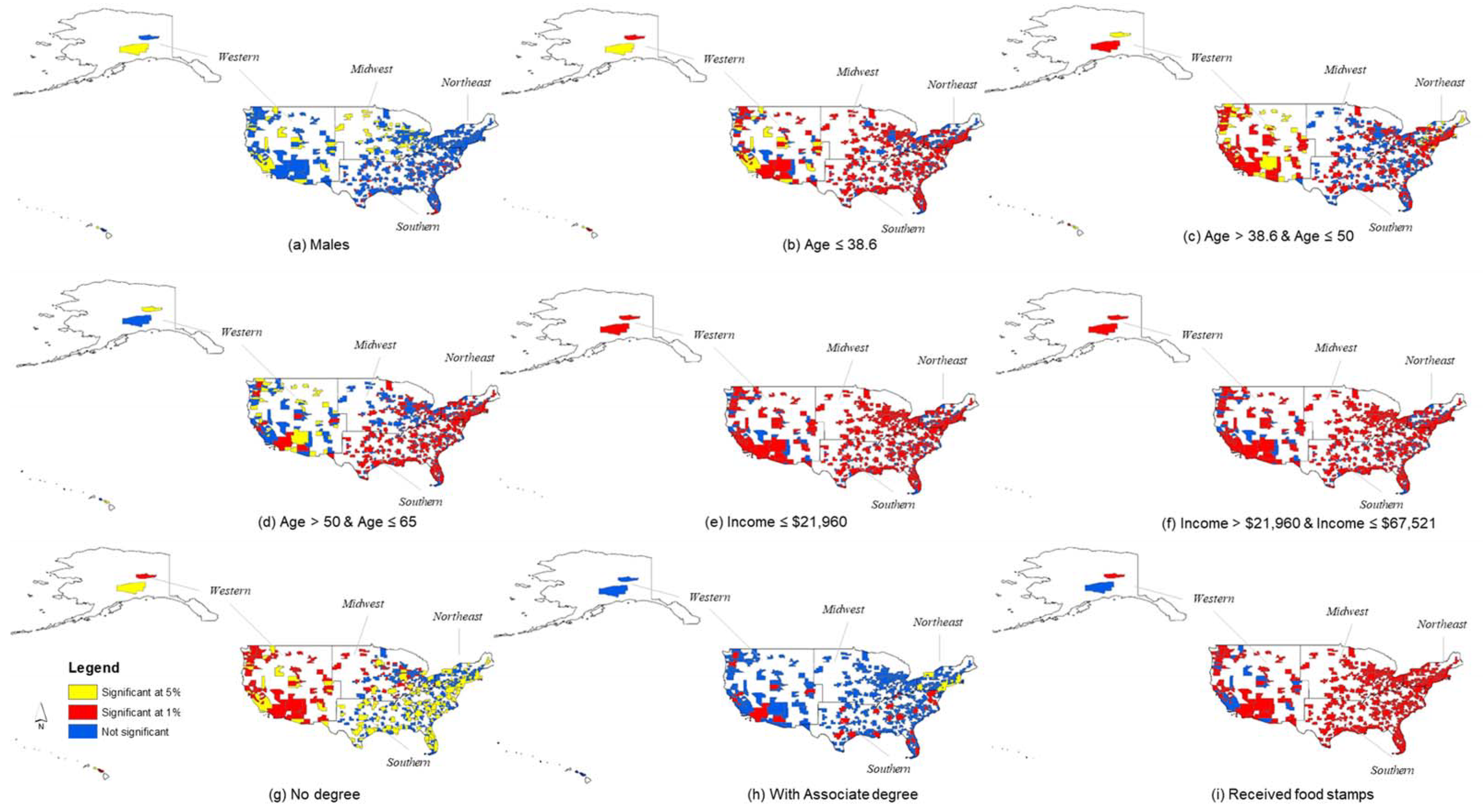
Spatial visualization of the significance of the estimates of the explanatory variables shown in Fig. 6 indicates that in most counties for males living near transit and respondents with an associate degree, food insecurity (whether positive or negative) largely remained undetermined at 1% and 5% significance level. This has been shown using blue shades (and few in yellow shades) in the maps of Figs. 6(a) and 6(h), with each shaded area representing a county. Food insecurity is significantly impacted in the Western counties, at 1% and 5% significance level, by the age of the respondents living near transit – as evident from the high number of red and yellow shaded clusters in the maps of Figs. 6(b) to 6(d). For other regions, this observation is noted at 1% significance level.
Similar observations are made of significant impacts in spatially clustered counties for the income and education level – evident from the maps in Figs. 6(e) to 6(h). Specifically, for those respondents living near transit with educational attainment with no degree, food insecurity is observed for both at 1% and 5% significance level for the counties in the Western states, shown in of Fig. 6(g).
As evident through red-shaded clustered counties of the map in Fig. 6(i), barring respondents from some counties in the Western States, all other respondents who reside near a transit across various counties of the four regions of aggregated states evidently exhibited food insecurity at 1% significance level with food stamps that were received in the last 12 months. This finding also points towards the fact that receiving food stamps or subscribing to SNAP does amount to food insecurity. Alternatively, from this finding, it could also be assumed that SNAP as a welfare scheme might not be working in dissipating food insecurity for those living near transit in the US. Further longitudinal studies need to be carried out to refute this assumption.
Thus, in summary, living near transit does not translate to food insecurity for the males only in a limited number of regions of the US. In addition, for certain age group, income-level, educational attainment, and subscription to food stamps or SNAP, food insecurity was prevalent among those living near transit in most of the four regions of the US.
Table 4. Coefficient estimates of explanatory variables (values in parenthesis are standard error).
Variables Northeast States Midwest States Southern States Western States
Large central metro Large fringe metro Medium and small metro Nonmetropolitan Large central metro Large fringe metro Medium and small metro Nonmetropolitan Large central metro Large fringe metro Medium and small metro Nonmetropolitan Large central metro Large fringe metro Medium and small metro Nonmetropolitan
Males -0.505* (0.223) 1.356 (0.658) -0.688* (0.306)
Age_386 0.79 (0.227) 0.933 (0.317) 1.482 (0.444) 0.803 (0.306) 1.578 (0.551) 0.923 (0.217) 0.71 (0.261) 0.749 (0.238) 0.513 (0.198) 1.228 (0.387) 1.123 (0.232)
Age_38650 1.101 (0.269) 1.792 (0.35) 1.824* (0.48) 1.484 (0.505) 1.839 (0.63) 1.205 (0.25) 0.597 (0.291) 0.854 (0.223) 1.325 (0.42) 1.334* (0.26) 1.588 (0.682)
Age_5065 0.661 (0.221) 1.081 (0.323) 0.975 (0.438) 1.32 (0.455) 1.119 (0.545) 0.967 (0.223) 0.891 (0.281) 0.897 (0.244) 0.611 (0.209) 1.106* (0.243)
Inc_p 2.454 (0.299) 2.636 (0.396) 2.188 (0.524) 1.863 (0.355) 1.904 (0.491) 2.209 (0.445) 2.707 (0.845) 2.239 (0.27) 1.824 (0.339) 2.679 (0.372) 1.906 (0.222) 3.204 (0.495) 1.918 (0.245)
Inc_pm 1.879 (0.273) 1.93 (0.296) 1.269 (0.465) 1.445 (0.3) 1.506 (0.38) 1.633 (0.418) 2.046 (0.794) 1.784 (0.241) 1.563 (0.254) 1.88 (0.351) 1.295 (0.185) 2.213 (0.416) 0.89 (0.202)
Edu_nd 0.692* (0.201) 1.05* (0.401) 0.866* (0.25) 1.343 (0.333) 0.800* (0.19) 0.753* (0.241) 0.739 (0.18) 0.855* (0.355) 0.731 (0.201) 1.365 (0.68)
Edu_ad 0.597* (0.305) 0.834 (0.235)
Food_S 1.095 (0.201) 1.086 (0.302) 2.168 (0.358) 2.571 (0.905) 1.759 (0.252) 1.872 (0.369) 1.401 (0.254) 1.149 (0.489) 1.055 (0.189) 1.434 (0.255) 1.47 (0.207) 1.514 (0.707) 1.315 (0.179) 0.984 (0.192) 1.874 (0.501)
* indicates 5% significance level, otherwise, all are 1% significance level
Table 5. Odds ratio for the explanatory variables
Variables Northeast States Midwest States Southern States Western States
Large central metro Large fringe metro Medium and small metro Nonmetropolitan Large central metro Large fringe metro Medium and small metro Nonmetropolitan Large central metro Large fringe metro Medium and small metro Nonmetropolitan Large central metro Large fringe metro Medium and small metro Nonmetropolitan
Males 0.605 4.05 0.501
Age_386 2.204 2.542 4.4 2.233 4.846 2.518 2.033 2.115 1.67 3.416 3.073
Age_38650 3.009 6 6.195 4.412 6.291 3.335 1.47 1.817 2.349 3.764 3.798 4.893
Age_5065 1.938 2.947 2.65 3.745 3.063 2.631 2.437 2.453 1.843 2.184 3.023
Inc_p 11.118 13.452 8.926 6.443 6.678 9.137 14.497 8.82 5.848 14.329 6.579 25.532 6.797
Inc_pm 6.228 6.809 3.577 4.242 4.488 5.132 7.577 5.867 4.684 6.61 3.613 9.17 2.439
Edu_nd 1.969 2.856 2.378 3.818 2.254 2.008 2.097 2.378 2.082 3.87
Edu_ad 1.867 2.329 2.294
Food_S 2.85 3.026 8.682 13.021 5.712 6.467 4.047 3.178 2.927 4.443 4.432 4.209 3.766 2.013 2.661 6.739
Figure 6. Spatial distribution of significant impacts of the explanatory variables (a)-(i) on food insecurity.
Preprints 82297 g006

Conclusion and Future Research

The findings in this paper point toward the growing need to promote policies that will reduce the need to use SNAP, especially for those populations residing near transit in the United States. This research evaluated food insecurity among the population residing close to transit. Data from the 2020 NHIS were analyzed to draw insights. A logistic regression analysis was carried out by treating food insecurity as the dependent variable and socioeconomic variables such as age, income, education and dependency on food stamps or SNAP as independent variables. Food insecurity is assessed with information on four aspects of inputs from those respondents who live close to transit, i.e. if they worried the food would run out, food didn't last, couldn’t afford to eat balanced meals, or had to cut the size of meals or skip meals.
Findings suggest that respondents who live close to transit in the US and are from large central metro counties of the Northeast, South and West states showed an increase in food insecurity if one or more of these three cases was true - i) if they were below 65 years of age, ii) had income below country’s median income, or iii) if their educational attainment was below bachelor’s degree. Further, a significant association was found between food insecurity of respondents living close to transit and the use of food stamps during the past twelve months across all the four regions of the aggregated states. This highlights that SNAP, a food program popular in the US, needs to be reviewed to ensure food security among Americans living close a transit.
The research findings suggest the need to improve transit connectivity to employment centers that can offer higher paying jobs than $67,521 per annum to males (below 65 years of age) possessing degrees below a bachelor’s.
In general, policies that would alleviate food insecurity among those living close to transit (as it is considered a cheaper mode of transportation, hence popular among low-income households) could include - reduced rental or property taxes in their existing location, welfare schemes (such as subsidized education expenses to earn a degree) and introduce incentives to access to jobs using transit as a readily available mode to achieve a sustained level of income much above the poverty threshold in the USA.
One of the major limitations of this research is that the results are presented based on the data that were available through the 2020 NHIS, and which might not be statistically sufficient. At the same time, the data were collected at the time of COVID-19 when only remote methods (such as phone interview, email etc.) could be only deployed and trusted. We hope to receive similar transit -related data and information on those living close to the transit so that a longitudinal study can be carried out to study the impacts of variables on food insecurity. Our future research will also involve identifying best practices related to these recommendations (and others) through example case studies from across the globe.

Funding

This research received no external funding

Institutional Review Board Statement

Not applicable

Informed Consent Statement

Not applicable

Data Availability Statement

Data supporting reported results can be found at Centers for Disease Control and Prevention (CDC) from the National Health Interview Survey (NHIS), https://www.cdc.gov/nchs/nhis/2020nhis.htm

Acknowledgments

None

Conflicts of Interest

The authors declare no conflict of interest

References

  1. 2013 National Center for Health Statistics (NCHS) Urban–Rural Classification Scheme for Counties, https://www.cdc.gov/nchs/data/series/sr_02/sr02_166.pdf (accessed on 4 May 2022).
  2. National Health Interview Survey (NHIS), 2020, https://ftp.cdc.gov/pub/Health_Statistics/NCHS/Dataset_Documentation/NHIS/2020/srvydesc-508.pdf (accessed on 1 May 2022).
  3. Poverty income threshold of $21,960 for a family size of 3: https://www.statista.com/statistics/183657/average-size-of-a-family-in-the-us/.
  4. US Department of Health and Human Services 2021, https://aspe.hhs.gov/topics/poverty-economic-mobility/poverty-guidelines/prior-hhs-poverty-guidelines-federal-register-references/2021-poverty-guidelines.
  5. Statistica.com, https://www.statista.com/statistics/241494/median-age-of-the-us-population/ (accessed on 5 January 2021).
  6. United States Department of Agriculture (USDA), Food and Nutrition Service, United States Department of Agriculture (USDA), https://www.fns.usda.gov/pd/snap-state-activity-reports (accessed on 22 April 2023).
  7. Pruitt, S., Leonard, T., Xuan, L., Amory, R., Higashi, R., Nguyen, O., & Swales, S. (2016). Who is food insecure? Implications for targeted recruitment and outreach, National Health and Nutrition Examination Survey, 2005–2010. Retrieved June 6, 2018. [CrossRef]
  8. Larson, J. ; Moseley, W. G. Reaching the limits: a geographic approach for understanding food insecurity and household hunger mitigation strategies in Minneapolis-Saint Paul, USA. GeoJournal, 2012; 77, 1-12. [CrossRef]
  9. Feeding America, https://map.feedingamerica.org/?_ga=2.156318203.1397879697.1691855096-248042924.1691855096 (accessed on August 10, 2023).
  10. Coleman-Jensen, A., Rabbitt, M. P., Gregory, C. A., & Singh, A. (2022). Household food security in the United States in 2021. Economic Research Report Number 309, US Department of Agriculture, accessed on July 23, 2023, https://www.ers.usda.gov/webdocs/publications/104656/err-309.pdf.
  11. International Food Policy Research Institute (IFPRI). https://www.ifpri.org/topic/food-security (accessed on 25 April 2022).
  12. HungerMap, World Food Programme (WFP), https://static.hungermapdata.org/insight-reports/2022-04-25/rbbsummary.pdf (accessed on 25 April 2022).
  13. Prosekov, A. Y.; Ivanova, S. A. Food security: The challenge of the present. Geoforum, 2018; 91, 73-77. [CrossRef]
  14. SNAP Eligibility, Food and Nutrition Service, United States Department of Agriculture, https://www.fns.usda.gov/snap/recipient/eligibility, (accessed on 21 May 2022).
  15. Welch, T. F. Equity in transport: The distribution of transit access and connectivity among affordable housing units. Transport policy, 2013; 30, 283-293. [CrossRef]
  16. Wang, K.; Woo, M. The relationship between transit rich neighborhoods and transit ridership: Evidence from the decentralization of poverty. Applied Geography, 2017; 86, 183-196. [CrossRef]
  17. Liang, C.;Huang, Y.; Yip, T. L.; Li, V. J. . Does rail transit development gentrify neighborhoods? Evidence from Hong Kong. Transportation Research Part A: Policy and Practice, 2022; 155, 354-372. [CrossRef]
  18. Derakhti, L.; Baeten, G. Contradictions of transit-oriented development in low-income neighborhoods: The case study of Rosengård in Malmö, Sweden. Urban Science, 2020; 4(2), 20.
  19. Gupta, S., “How can Delhi provide affordable housing near transit to its poor”, DownToEarth, https://www.downtoearth.org.in/blog/governance/how-can-delhi-provide-affordable-housing-near-transit-to-its-poor-73619 (accessed on 11 May 2022).
  20. Sharp, S. “Affordable Housing Rises Next to Blue Line in Long Beach”, Urbanize Los Angeles, 2018, “Affhttps://la.urbanize.city/post/affordable-housing-rises-next-blue-line-long-beach (accessed on 4 May 2022).
  21. Burrows, M.; Burd, C.; McKenzie, B. Commuting by public transportation in the United States: 2019. American Community Survey Reports 2021, 802.
  22. Baek, D., 2016. The effect of public transportation accessibility on food insecurity. Eastern Economic Journal, 2016; 42(1), 104-134.
  23. Gundersen, C.; Kreider, B.; Pepper, J. The economics of food insecurity in the United States. Applied Economic Perspectives and Policy, 2011; 33(3), 281-303. [CrossRef]
  24. Baek, D. (2014). Essays on Poverty and Infant Health. Louisiana State University and Agricultural & Mechanical College.
  25. Martinez, J. C.; Clark, J. M.; Gudzune, K. A. Association of personal vehicle access with lifestyle habits and food insecurity among public housing residents. Preventive medicine reports, 2019; 13, 341-345. [CrossRef]
  26. Swayne, M. R., & Lowery, B. C. (2021). Integrating transit data and travel time into food security analysis: A case study of San Diego, California. Applied Geography, 131, 102461. [CrossRef]
  27. Spencer, M., Petteway, R., Bacetti, L., Barbot, O., 2011. Healthy Baltimore 2015, 1st ed. Baltimore City Health Department, Baltimore City. http://health.baltimorecity.gov/ sites/default/files/HealthyBaltimore2015_Final_Web.pdf, (accessed on 10 August 2023).
  28. Patil, G. R. ; Sharma, G. Overweight/obesity relationship with travel patterns, socioeconomic characteristics, and built environment. Journal of Transport & Health, 2021; 22, 101240. [CrossRef]
Disclaimer/Publisher’s Note: The statements, opinions and data contained in all publications are solely those of the individual author(s) and contributor(s) and not of MDPI and/or the editor(s). MDPI and/or the editor(s) disclaim responsibility for any injury to people or property resulting from any ideas, methods, instructions or products referred to in the content.
Copyright: This open access article is published under a Creative Commons CC BY 4.0 license, which permit the free download, distribution, and reuse, provided that the author and preprint are cited in any reuse.
Prerpints.org logo

Preprints.org is a free preprint server supported by MDPI in Basel, Switzerland.

Subscribe

© 2024 MDPI (Basel, Switzerland) unless otherwise stated